American Journal of Engineering Research (AJER) 2016 American Journal of Engineering Research (AJER) e-ISSN: 2320-0847 p-ISSN : 2320-0936 Volume-5, Issue-5, pp-190-197 www.ajer.org Research Paper
Open Access
Free Vibration Analysis of an Alround-Clamped Rectangular Thin Orthotropic Plate Using Taylor-Mclaurin Shape Function D.O Onwuka1, O.M Ibearugbulem2, A.C Abamara3, C.F Njoku4, S.I Agbo5 1, 2, 4, 5
(Department of Civil Engineering, Federal University of Technology, Oweeri Nigeria) 3 (Federal Ministry of Transport, Abuja, Nigeria)
ABSTRACT:A comprehensive free vibration analysis of an alround-clamped rectangular thin or thotropic plate, was carried out using Taylor- Mclaurin shape function, and Ritz method. The Taylor-Mclaurin shape function truncated at the fourth term satisfied all the boundary conditions of the alround-clamped thin orthotropic plate. The shape function was substituted into the total energy functional, which was subsequently minimized. From the minimized equation, the natural frequency equation for the clamped plate, was derived. The resulting equation was used to calculate fundamental natural frequencies of the clamped plate for various aspect ratios, p and different combinations of flexural rigidity ratios, φ. The fundamental frequencies for a clamped plate vibrating in the first mode are given in Tables1-5, for different flexural rigidities, φ and aspect ratios varying from 0.1 to 2 at increments of 0.1. The average percentage difference in the values of natural frequency for the flexural rigidity ratios, φ1, φ2, and φ3, are 1.532%,1.367% and 1.425% for different values of đ?‘? đ?‘Ž the aspect ratio, đ?‘? = ; and 1.149%, 1.506% and‌‌..for different values of the aspect ratio,đ?‘? = . đ?‘Ž đ?‘? These average percentage differences indicate that the formulated deflection function for the clamped plate, is a very good approximation to the exact deflection function of the free vibration of a clamped rectangular thin orthotropic plate. Keywords:Clamped rectangular plate, free vibration analysis, natural frequency, orthotropic vibrating plate, Taylor-Mclaurin method, shape function.
I.
INTRODUCTION
Orthotropic plates are commonly used in the fields of structural engineering and are considered to be fundamental structural elements in aerospace, naval and ocean structures [1], [2],[3].The governing equation for free vibration of thin rectangular plates, isa fourth order differential equation and the determination of the exact solution of a clamped plate by direct integration, is not possible. Some of the works on this subject were carried out using other approaches such as numerical and variational methods, which are approximate methods. [4] Used the Rayleigh-Ritz method and made some useful contributions. [5] Presented and used Rayleigh- Ritz method and decomposition technique, to evaluate the upper and lower bounds of vibration frequencies for an alround-clamped rectangular orthotropic plate. [6], first used a method based on superposition of the appropriate Levy type of solutions, for the analysis of rectangular plates. Gorman, further applied this method by Timoshenko and Krieger, to the free vibration analyses of isotropic plate, [7], thereafter to clamped orthotropic plate [8], then to free orthotropic plate, [9]. And finally to point supported or thotropic plates [10]. Before now, it was believed that the exact solution of free vibration of an alround-clamped orthotropic plate was not achievable until [11] used novel separation of variable to obtain the exact solutions for free vibrations of rectangular thin orthotropic plates with all combinations of simply supported and clamped boundary conditions. As a matter of fact, the equation by [12], was used for calculating the radian natural frequency of a deformed orthotropic vibrating plate. One of the plate cases considered, is the alround-clamped plate.Solutions for an alround-clamped plate, were obtained for the first time, even though, it was originally believed it was not obtainable. He alsovalidated the results from his work by extensive comparison with results from finite element method and other numerical methods available in literature. The new exact solution provided values for other researchers that used approximate methods, to compare their results with. It is noteworthy, that none of the researchers, has used the Taylor-Mclaurin series in Rayleigh-Ritz method, to evaluate approximate solutions of alround-clamped orthotropic rectangular thin plates, and the object of this study is to fill that gap.
www.ajer.org
Page 190
American Journal of Engineering Research (AJER)
2016
II. MATHEMATICALFORMULATION 2.1. Governing Differential Equation of a Thin Plate in Vibration. In 2001, [13] derived the fourth-order homogenous partial differential equation governing the undamped, free, linear vibration of plates as follows: ∂2 w D∇2 ∇2 w x, y, t + ρh 2 x, y, t = 0 (1) ∂t 2 ∂ w D∇4 w x, y, t + ρh 2 x, y, t = 0 (2) ∂t where ∂4 ∂4 ∂2 w ∇4 = 4 + 2 2 2 + ρh 2 x, y, t = 0 (3) ∂x ∂x dy ∂t D = flexural rigidity of the plate w(x, y, t) = deflection of the plate x = Cartesian co-ordinate in the horizontal direction y = Cartesian co-ordinate in the vertical direction t = thickness of the plate. ρ =density of the material m= mass 2.2. Truncated Taylor Maclaurin Series. [14]Expanded the general shape function using the Taylor-Maclaurin series and obtained equation (4) ∞ ∞ F m x F n y 0 0 w = w x, y = (x − x0 )m . (y − y0 )n (4) m! n! m=0 n=0 whereF m x0 is the mthpartial derivative of the function, w, with respect to x and F n y0 is the th n partial derivative of the function, w with respect to y. And m! and n! are the factorials of m and n respectively, while x0 and y0 are the points of origin. He truncated the infinite series at m= n =4 and gave shape function as: 4
4
m =0
n=0
w=
Im Jn x m . y n
(5)
Transforming the x-y co-ordinate system to R-Q coordinate system, yielded x y R = and Q = , where R and Q are dimensionless quantities. a b Since x = aR and y – bQ and letting am = Im.am and bn = Jn.bn, Equation (5) reduces to Equation(6). 4
4
m =0
n=0
w=
a m bn Rm Qn
The function given by Equation (6) can be further expanded in the following form: w R, Q = a 0 + a1 R + a 2 R2 + a 3 R3 + a 4 R4 b0 + b1 Q + b2 Q2 + b3 Q3 + b4 Q4 Whereai and bi (i= 0,1,2,3 and 4) are unknown constants of the shape function series. Here, the Equation (7) is truncated at M=N=4.
(6) (7)
2.3. Boundary Conditions for an Alround Clamped Plate. Consider a rectangular plate: which is clamped on all edges as shown in Fig 1:
From Fig 1, the boundary conditions for the orthotropic rectangular plate clamped on all 4 edges and represented by CCCC are: W R=0 =0 (8) W R=1 =0 (9)
www.ajer.org
Page 191
American Journal of Engineering Research (AJER)
2016
W Q=0 =0 (10) W Q=1 =0 (11) W ′R R = 0 = 0 (12) W ′R R = 1 = 0 (13) W ′Q Q = 0 = 0 (14) W ′Q Q = 1 = 0 (15) whereW ′R and W ′Q are the first derivatives of the displacement functions with respect to the R and Q directions respectively. Substituting successively, the boundary conditions, namely, W R = 0 = 0; W ′R R = 0 = 0 ,W Q = 0 = 0, and W ′Q Q = 0 = 0 into the Equation (7), yields respectively. a0 = 0 (16) a1 = 0 (17) b0 = 0 (18) b1 = 0 (19) And, substituting the other boundary conditions, viz, W Q = 1 = 0 and W ′Q Q = 1 = 0 into Equation (7) one after the other, gives respectively: a2+ a3 +a4 = 0 (20) 2a2+ 3a3 +4a4 = 0 (21) Solving simultaneously yields a2= a4, and a3=2a4 (22) Also, substituting the boundary conditions, W Q = 1 = 0 and W ′Q Q = 1 = 0 one after the other, into Equation (7) and solving the simultaneous equation gives: b2= b4, and b3 = -2b4 Substituting the constants, a0, a1, a2, a3, a4, b0, b1, b2, b3, and b4 into Equation (7) gives the deflection function, w, as follows: W= A (R2-2R3+R4) (Q2-2Q3+Q4) (23a) =AH (23b) where A=a4b4 and H= (R2-2R3+R4) (Q2-2Q3+Q4) As a matter of fact, ‘A’ is the amplitude of the deflected shape while ‘H’ is the deflected shape.
NATURAL FREQUENCY EQUATION, Λ, FOR A VIBRATING ORTHOTROPIC PLATE.
III.
3.1. Formulation of the Natural Frequency Equation, λ, for a Free Vibrating Alround-clamped Rectangular Orthotropic Plate. Using a deflection function technique based on the work of [14], derived the equation for the fundamental frequency of a vibrating continuum. This was achieved by employing the principle of conservation of energy, in which the strain and kinetic energies of the continuum, were derived from the first principles using the theory of elasticity. The expressions were subsequently substituted into the potential energy functional, and then minimized to determine the fundamental frequency, that is, at mode M=N=1. Then, the fundamental frequency is made the subject of the equations after substituting the aspect ratios p=a/b and p=b/a, as the case may be. First, the strain energy, U, is given as: U=
D x 1 1 φ1 ∂ 2 w 2 [ ( ) 2b 2 0 0 p 3 R 2
+2
φ2 p
(
∂2w ∂R ∂Q
∂2w 2 ) ]∂R ∂Q ∂Q 2
)2 +pφ3 (
(24)
And the kinetic energy, K.E, is given as: pb 2 λ2 ρt
1
1
K.E= W 2 ∂R ∂Q 0 0 2 And total potential energy functional represented by the symbol, π is expressed by Equation (26) Π = U - K.E Substituting Equation (24 ) and (25 ) into Equation (26 ), yields, Equation (27) Π=
Dx 2b 2
φ2 ∂ 2 w 2 1 1 φ1 ∂ 2 w 2 [ ( ) +2 ( ) 3 2 0 0 p R p ∂R ∂Q
∂2w 2 pb 2 λ2 ρt 1 1 ) ]∂R ∂Q W2 2 0 0 ∂Q 2
+pφ3 (
∂R ∂Q
(25)
(26) (27)
Since the deflection function, W = AH, the Equation (27) becomes: Π=
Dx A2 2b 2
φ2 ∂ 2 H 2 1 1 φ1 ∂ 2 H 2 [ ( ) +2 ( ) 3 2 0 0 p ∂R p ∂R ∂Q
+pφ3 (
∂2 H 2 pA 2 b 2 λ2 ρt 1 1 2 ) ]∂R ∂Q H 2 0 0 ∂Q 2
∂R ∂Q
(28)
Minimizing this Equation (28) gives: ∂Π D x A ∂A
=
b2
φ 1 1 φ1 ∂ 2 H 2 ∂2H 2 [ ( ) +2 2 ( ) 0 0 p 3 ∂R 2 p ∂R ∂Q
www.ajer.org
∂2H 2 ) ]∂R ∂Q ∂Q 2
+pφ3 (
-pAb2 λ2 ρt
1 1 2 H 0 0
∂R ∂Q = 0
(29)
Page 192
American Journal of Engineering Research (AJER)
2016
At this point, the natural frequency squared,λ2 is made the subject of the Equation (29). For the aspect ratio, p=a/b,λ2 can be expressed in terms of φ and b as follows: φ D x A 1 1 φ1 ∂ 2 H 2 ∂2 H 2 ∂2H [ ( ) +2 22 ( ) +pφ3 ( 2 )2 ] ∂R ∂Q b 4 ρt 0 0 p 4 ∂R 2 p ∂R ∂Q ∂Q 1 1 2 H ∂R ∂Q 0 0
2
λ =
(30)
In terms of a and b, Equation (30) becomes: λ2 =
∂2 H ∂2 H 2 φ3 a 4 ( 2 )2 2φ2 a 2 ( ) Dx 1 1 ∂2 H 2 ∂R ∂Q ∂Q [φ ( ) + + ] ∂R ∂Q a 4 ρt 0 0 1 ∂R 2 b2 b4 1 1 2 0 0 H ∂R ∂Q
(31)
2
In terms of p and a, the same expression for λ ,becomes: Dx 1 1 ∂2 H 2 ∂2H 2 ∂2H [φ ( ) +2φ2 p 2 ( ) +pφ3 p 4 ( 2 )2 ] ∂R ∂Q ∂R ∂Q a 4 ρt 0 0 1 ∂R 2 ∂Q 1 1 2 0 0 H ∂R ∂Q
2
λ =
(32)
Similarly, for aspect ratio p = b/a, the expression for natural frequency squared,λ2 in terms of a and p, is given as follows: Dx A 1 1 ∂2H 2 [φ ( ) a 4 ρt 0 0 1 ∂R 2
λ2 =
+
∂2 H 2 2φ2 ( ) ∂R ∂Q + p2 1 1 2 0 0 H ∂R ∂Q
∂2 H φ3 a 4 ( 2 )2 ∂Q ] ∂R ∂Q p4
(33)
Where t, is the plate thickness, a and b are the length and width of the plate respectively. 3.2. Use of Rayleigh – Ritz Method to Determinethe Natural Frequency ,λ, of an Alround-Clamped Plate in Free Vibration. Let the partial differentials of the deflection functions, W, expressed in terms of dimensionless parameters R and Q, be as follows: ∂W(R,Q) W ′R = (34) W ′′R = W
′Q
=
W ′′Q =
∂R ∂ 2 W (R,Q)
(35)
∂R 2 ∂W (R,Q)
(36)
∂Q ∂ 2 W (R,Q)
W ′′RQ =
(37)
∂Q 2 ∂ 2 W (R,Q)
(38)
∂R ∂Q
where W=AH are as defined earlier. The parameters,W ′′R , W ′′Q , W ′′RQ , their squares and double integrals ,are evaluated with respect to R and Q as follows: 1 1 (W ′′R )2 = 2R ∂Q = A2 0.8 0.00159 = 0.00127A2 (39) 0 0 1 1 (W ′′Q )2 ∂R ∂Q = A2 0.00159 0.8 = 0.00127A2 0 0 1 1 (W ′′RQ )2 = 2R ∂Q = A2 0.01905 0.01905 = 0.00036A2 0 0 1 1 W 2 ∂R ∂Q = (0.0015873)2 = 0.000002519526329A2 0 0
(40) (41) (42)
Substituting these values into the natural frequency squared, λ2, equation, gives 2φ D x φ1 [ ∗0.00127 + 22 ∗0.00036 +φ3 ∗0.00127 ] b 4 ρt p 4 p
λ2 = for p= a/b 0.000002519526329 This expression further reduces to Equation (44) φ φ D λ2 = 4x [ 14 ∗ 503.9683 + 22 ∗ 285.714 + φ3 ∗ 503.9683] b ρt p
(43) (44)
p
Re-arranging the equation in terms of a and p, gives: D λ2 = 4 x [φ1 ∗ 503.9683 + φ2 ∗ 285.714p2 + φ3 ∗ 503.9683p4 ]
(45)
a ρt
2
Substituting a/b in place of p into Equation (32) yields the expression for λ in termsof a and b. λ2 =
2 2 2 ∂ H 2 p φ p 4 (∂ H )2 3 Dx 1 1 ∂ 2 H 2 2φ2 p (∂R ∂Q ) ∂Q 2 [φ ( ) + + ] ∂R ∂Q a 4 ρt 0 0 1 ∂R 2 b2 b4 1 1 2 H ∂R ∂Q 0 0
(46)
2
Therefore, the natural frequency squared, λ , equation in terms of aand b is given by: 2
2φ a 2 φ a4 Dx [φ ∗0.00127 + 22 ∗0.00036 + 3 4 ∗0.00127 ] b 4 ρt 1 b b
λ = 0.000002519526329 This can be simplified further to Equation (48)
www.ajer.org
(47)
Page 193
American Journal of Engineering Research (AJER) Îť2 =
Dx b 4 Ď t
[φ1 ∗ 503.9683 +
φ2 a 2 b2
∗ 285.714 +
φ3 a 4 b4
2016
∗ 503.9683]
(48)
When aspect ratio, p=b/a, (i.e. reciprocal of a/b), is substituted into the expression, then Equation (45) becomes: φ φ D Îť2 = 4 x [φ1 ∗ 503.9683 + 22 ∗ 285.714 + 34 ∗ 503.9683] (49) a Ď t
p
p
IV.
RESULTS AND DISCUSSION
The equation for natural frequency, Îť, of a free vibrating rectangular orthotropic plate clamped on all edges, can be obtained from the square roots of Equation (45) and Equation (49) for aspect ratios, p=a/b and p= b/a respectively. Îť= Îť=
Dx a 4 Ď t Dx a 4 Ď t
[φ1 ∗ 503.9683 + φ2 ∗ 285.714p2 + φ3 ∗ 503.9683p4 ]
[φ1 ∗ 503.9683 +
φ2 p2
∗ 285.714 +
φ3 p4
(50)
∗ 503.9683]
(51)
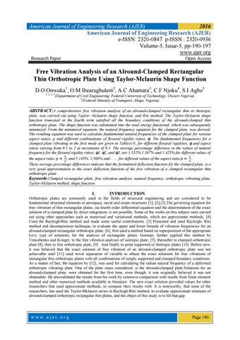
These equations were used to calculate the natural frequencies of a free vibrating thin rectangular orthotropic plate clamped on all edges for various aspect ratios, p=b/a and p= a/b and various combinations of flexural rigidities, φ1 ,φ2 and φ3 . The results are shown in Tables 1-5. In addition, graphs of natural frequencies, Ν, against aspect ratios, p=b/a, were plotted for various combinations of flexural rigidity,φ1 ,φ2 and φ3 (see Fig 2)The values of natural frequencies, Ν, obtained in this work, were compared withboth the corresponding exact solutions by [11] and solutions by Kantorovich in Tables 1-5. As shown in Tables 1-3, the percentage differences between the natural frequencies obtained in this work and those of [11], range from 1.367 percent to1.532 percent for different aspect ratios, p=b/a.Both results tend to converge as the aspect ratio, p, increase, but diverges as the aspect ratio, p decreases. Similar comparison indicates higher convergence between the results of the present work and those of Kantorovich. Table 1: Flexural rigidities, φ1 =φ2 =φ3 =1, and aspect ratio p =
đ?‘? đ?‘Ž
S/N
P
đ?›Œ2
Îť 1 (Pred)
Îť 2 (Liu)
Îť 3 (Kant)
đ?›Œđ?&#x;?– đ?›Œđ?&#x;? ∗ đ?&#x;?đ?&#x;Žđ?&#x;Ž% đ?›Œđ?&#x;?
1 2 3 4 5 6 7 8 9
0.1 0.2 0.3 0.4 0.5 0.6 0.7 0.8 0.9
5068758 322627 65896.88 21975.94 9710.317 5186.263 3186.051 2180.788 1624.829
2251.390 568.003 256.704 148.243 98.541 72.016 56.445 46.699 40.309
97.542
98.324
1.014
0.220
10 11 12 13 14 15 16 17 18 19 20
1.0 1.1 1.2 1.3 1.4 1.5 1.6 1.7 1.8 1.9 2.0
1293.651 1084.313 945.4211 849.4831 780.9278 730.5016 692.4748 663.1716 640.1596 621.7848 606.8948
35.967 32.929 30.748 29.146 27.945 27.028 26.315 25.752 25.301 24.936 24.635
35.112
35.999
2.377
0.089
24.358
24.581
1.124
0.219
đ?›Œđ?&#x;?– đ?›Œđ?&#x;‘ ∗ đ?&#x;?đ?&#x;Žđ?&#x;Ž% đ?›Œđ?&#x;?
Ν1(Pred) – Result obtained from the formulated Ν2 (Liu) – Liu and Xing (2008) solution Ν3 (Kant) – Kantorovich solution Table 2: Flexural rigidities, φ1 = 1, φ2 = 0.5, φ3 =1, and aspect ratio p = S/N
P
đ?›Œ2
Îť 1 (Pred)
1 2 3 4 5 6
0.1 0.2 0.3 0.4 0.5 0.6
5054473 319055.6 64309.58 21083.09 9138.889 4789.438
2248.215 564.850 253.593 145.200 95.598 69.206
www.ajer.org
Îť 2 (Liu)
Îť 3 (Kant)
đ?›Œđ?&#x;?– đ?›Œđ?&#x;? ∗ đ?&#x;?đ?&#x;Žđ?&#x;Ž% đ?›Œđ?&#x;?
94.725
95.391
0.913
đ?‘? đ?‘Ž
đ?›Œđ?&#x;?– đ?›Œđ?&#x;‘ ∗ đ?&#x;?đ?&#x;Žđ?&#x;Ž% đ?›Œđ?&#x;?
0.217
Page 194
American Journal of Engineering Research (AJER) 7 8 9 10 11 12 13 14 15 16 17 18 19 20
0.7 0.8 0.9 1.0 1.1 1.2 1.3 1.4 1.5 1.6 1.7 1.8 1.9 2.0
2894.507 1957.574 1448.462 1150.794 966.2491 846.2148 764.9524 708.0416 667.0096 636.6713 613.7401 596.0679 582.2122 571.1806
53.801 44.244 38.059 33.923 31.085 29.090 27.658 26.609 25.827 25.232 24.774 24.415 24.129 23.899
2016
33.174
33.917
2.208
0.018
23.681
23.848
0.912
0.213
Ν1(Pred) – Result obtained from the formulated Ν2 (Liu) – Liu and Xing (2008) solution Ν3 (Kant) – Kantorovich solution Table 3: Flexural rigidities, φ1 = 1, φ2 = 0.5, φ3 = 0.5, and aspect ratio p = S/N
P
đ?›Œ2
Îť 1 (Pred)
1 2 3 4 5 6 7 8 9 10 11 12 13 14 15 16 17 18 19 20
0.1 0.2 0.3 0.4 0.5 0.6 0.7 0.8 0.9 1.0 1.1 1.2 1.3 1.4 1.5 1.6 1.7 1.8 1.9 2.0
2534631 161565.5 33200.42 11239.96 5107.143 2845.115 1845.01 1342.378 1064.399 898.8095 794.1405 724.6947 676.7257 642.4481 617.2349 598.2215 583.5699 572.0639 562.8765 555.4316
1592.053 401.952 182.210 106.019 71.464 53.340 42.954 36.638 32.625 29.980 28.180 26.920 26.014 25.347 24.844 24.459 24.157 23.918 23.725 23.568
Îť 2 (Liu)
Îť 3 (Kant)
đ?›Œđ?&#x;?– đ?›Œđ?&#x;? ∗ đ?&#x;?đ?&#x;Žđ?&#x;Ž% đ?›Œđ?&#x;?
70.524
71.371
1.315
0.130
29.329
29.986
2.171
0.020
23.399
23.504
0.717
0.272
đ?‘? đ?‘Ž
đ?›Œđ?&#x;?– đ?›Œđ?&#x;‘ ∗ đ?&#x;?đ?&#x;Žđ?&#x;Ž% đ?›Œđ?&#x;?
Ν1(Pred) – Result obtained from the formulated Ν2 (Liu) – Liu and Xing (2008) solution Ν3 (Kant) – Kantorovich solution � Table 4: Flexural rigidities, φ1 = 1, φ2 = 0.648088, φ3 = 3.117304 and aspect ratio p = S/N
P
đ?›Œ2
1 2 3 4 5 6 7 8 9 10 11 12 13 14 15 16 17 18 19 20
0.1 0.2 0.3 0.4 0.5 0.6 0.7 0.8 0.9 1.0 1.1 1.2 1.3 1.4 1.5 1.6 1.7 1.8 1.9 2.0
505.9771 513.8887 533.3587 573.8134 648.4492 774.2333 971.9031 1265.967 1684.702 2260.159 3028.155 4028.282 5303.899 6902.137 8873.897 11273.85 14160.44 17595.88 21646.15 26381
www.ajer.org
Îť 1 (Pred ) 22.494 22.669 23.095 23.954 25.465 27.825 31.175 35.580 41.04 47.541 55.029 63.469 72.828 83.079 94.201 106.178 118.998 132.649 147.126 162.422
đ?‘?
Îť 2 (Liu)
Îť 3 (Kant)
đ?›Œđ?&#x;?– đ?›Œđ?&#x;? ∗ đ?&#x;?đ?&#x;Žđ?&#x;Ž% đ?›Œđ?&#x;?
đ?›Œđ?&#x;?– đ?›Œđ?&#x;‘ ∗ đ?&#x;?đ?&#x;Žđ?&#x;Ž% đ?›Œđ?&#x;?
25.104
25.424
1.418
0.161
46.741
47.481
1.683
0.126
93.378
93.980
0.874
0.235
161.51
161.95
0.562
0.291
Page 195
American Journal of Engineering Research (AJER)
2016
Ν1(Pred) – Result obtained from the formulated Ν2 (Liu) – Liu and Xing (2008) solution Ν3 (Kant) – Kantorovich solution Table 5: Flexural rigidities, φ1 = 1, φ2 = 0.232019, φ3 = 0.070766, and aspect ratio p = S/N
P
đ?›Œ2
1 2 3 4 5 6 7 8 9 10 11 12 13 14 15 16 17 18 19 20
0.1 0.2 0.3 0.4 0.5 0.6 0.7 0.8 0.9 1.0 1.1 1.2 1.3 1.4 1.5 1.6 1.7 1.8 1.9 2.0
504.6348 506.677 510.2234 515.4879 522.7701 532.4551 545.0138 561.0025 581.0632 605.9233 636.396 673.38 717.8598 770.9051 833.6715 907.400 993.4175 1093.136 1208.054 1339.754
Îť 1 (Pred ) 22.464 22.509 22.588 22.704 22.864 23.075 23.346 23.685 24.105 24.616 25.227 25.950 26.793 27.765 28.873 30.123 31.517 33.063 34.757 36.603
Îť 2 (Liu)
Îť 3 (Kant)
đ?›Œđ?&#x;?– đ?›Œđ?&#x;? ∗ đ?&#x;?đ?&#x;Žđ?&#x;Ž% đ?›Œđ?&#x;?
22.757
22.780
0.468
0.367
24.358
24.564
01.158
0.211
28.289
28.869
2.023
0.014
35.735
36.618
2.371
0.041
đ?‘? đ?‘Ž
đ?›Œđ?&#x;?– đ?›Œđ?&#x;‘ ∗ đ?&#x;?đ?&#x;Žđ?&#x;Ž% đ?›Œđ?&#x;?
Ν1(Pred) – Result obtained from the formulated Ν2 (Liu) – Liu and Xing (2008) solution Ν3 (Kant) – Kantorovich solution
Figure2.
V.
CONCLUSION
The fully restrained or (clamped) (CCCC) plates, yielded higher natural frequencies than alround- simply supported (SSSS) plates. Besides, the convergence of the graph/results, present solution with the exact solution, of plates, shows that the present solution approximates closely than the exact solution. It can also be concluded that the use of Taylor series (which overcomes the deficiencies or limitations of other methods), is more effective in approximating deformed shape of alround clamped thin rectangular orthotropic plate undergoing free vibration. Thus, fully restrained free vibrating plates can simply be analyzed using the newly developed method in this work.
www.ajer.org
Page 196
American Journal of Engineering Research (AJER)
2016
REFERENCES [1]. [2]. [3]. [4]. [5]. [6]. [7]. [8]. [9]. [10]. [11].
[12]. [13]. [14].
Biancolini, M. E., Brutti C and RecciaL(2005) Approximate Solution for Free Vibrations of Thin Orthotropic Rectangular Plates. J Sound Vib; 288; 3 21-44. Rossi, R. E, Bambill, D. V and Laura P.A.A(1998) Vibrations of a Rectangular Orthotropic Plate with a Free Edge: Comparison of Analytical and Numerical Results. Ocean Eng, 25 (7); 521-7. Chen, W.Q and Lue,C.F 3D(2005) Free Vibration Analysis of Cross-Ply Laminated Plates with One Pair of Opposite Edges Simply Supported. Compos Struct; 69, 77-87. Marangoni, R.D, Cook, L.M and Basavanhally, N (1978) Upper and Lower Bounds to the Natural Frequencies of Vibration of Clamped Rectangular Orthotropic plates.Int J Solids Struct; 14; 6 11-23. Bazely,N.W, Fox DW and Stadter, JT(1965) Upper and Lowre Bounds for Frequencies of Rectangular Clamped Plates. Applied Physics Laboratory, Technical Memo, TG-626.The John Hopkins University, Baltimore. Timoshenko, S P and Krieger,S W(1959) Theory of Plates and Shells. Tokyo: McGraw-Hill. Gorman, D. J. (1982). Free Vibration Analysis of Rectangular Plates. New York: Elsevier, North Holland. Gorman, D. J (1990) Accurate Free Vibration Analysis of Clamped Orthotropic plates by the Method of Superposition .J Sound Vib 140 (3):391-411 Gorman, D. J, Wei, D. (2003) Accurate Free Vibration Analysis of Completely Free Symmetric Cross-ply Rectangular Laminated Plates. Compos struct;60:359-65. Gorman, D. J. (1994) Free Vibration Analysis of Point Supported Orthotropic Plates. J Eng. Mech; 120 (1): 58-74. Xing, Y. F, Liu, B. (2008). New Exact Solutions for Free Vibrations of Thin Orthotropic Rectangular Plates, The Solid Mechanics Reserch Center, Beijing University of Aeronautics and Astronautics, Beijing 100083, China. Composite Structures Jornal Homepage: www.elsevier.com/locate/compstruct. Chakraverty, S., (2009). Vibration of Plates, New York: CRC Press. Ventsel, E. and Krauthammer, T. (2001). Thin Plates and Shell (Theory, Analysis and Applications). New York: Marcel Dekker. Ibearugbulem, O.M.(2013) Application of a Direct Variational Principle in Elastic Stability Analysis of thin Rectangular Isotropic Plates. A PhD Thesis submitted to Federal University of Technology, Owerri.
www.ajer.org
Page 197