WATER RESOURCES PLANNING AND MANAGEMENT
2.1 The Internet is an excellent source of information on this topic. The level of integrated water resources management varies by state.
2.2 Virtually all of the laws listed in Table 2.1 provide some protection for preventing and controlling water pollution. Information on each law may be found on the Internet. It is also important to note that the EPA only regulates at the Federal level and much of the cleanup and protection is now delegated to states and local governments.
2.3 Point source pollution = Pollution that originates at one location with discrete discharge points. Typical examples include industrial and wastewater treatment facilities. Nonpoint source pollution = Pollution that is usually input into the environment in a dispersed manner. Typical examples include stormwater runoff that contains fertilizers, pesticides, herbicides, oils, grease, bacteria, viruses, and salts.
2.4 Adverse health effects of toxic pollutants are numerous and can include a variety of conditions. Some pollutant-related conditions include asthma, nausea, and various cancers among many others.
2.5 Agencies that are responsible for water quantity and quality significantly vary by state.
2.6 This is a subjective question and one that has been and will continue to be debated in the water resources community.
2.7 Integrated water resources management is difficult to achieve because it involves both a financial and resources investment over time. It is also important to obtain concensus on this approach from all of the involved stakeholders. This difficulty is perhaps why there are so few examples of true integrated water resources management.
2.8 This question is subjective but the student should research specific examples to support their argument.
CHAPTER 3
THE HYDROLOGIC CYCLE AND NATURAL WATER SOURCES
3.1 The answer to this question will vary by location.
3.2 reservoir area = 3900/640 = 6.1 sq. mi.
annual runoff = (14/12)(190 – 6.1)(640) = 137,704 ac-ft
annual evaporation = (49/12)(3900) = 15,925 ac-ft
draft = (100 X 365 X 106)/(7.48 X 43,560) = 112,022 ac-ft
precipitation on lake = (40/12)(3900) = 13,000 ac-ft
gain in storage = 137,704 + 13,000 = 150,704
loss in storage = 112,022 + 15,925 = 127,947
net gain in storage = 22,757 ac-ft
3.3 reservoir area = 1700 hec = 17 X 106 sq. meters annual runoff = 0.3(500 X 10
3.4 To complete a water budget, it is first important to understand how the water budget will be used and what time step will be necessary to successfully model the system. Once the budget is conceptually designed, a variety of online sources can usually be used to collect the data. These sources include but are not limited to:
state regulatory agencies
special water districts
weather agencies,
local governments
geological surveys
agricultural agencies
Historical data and previous reports can also yield important information on the system. Verification and calibration data should also be considered as part of the data collection effort.
3.5 The solution for this problem will vary based on location.
6 – 17 X 106) = 144 X 106 sq.
17 X 106 = 20.4 X 10⁶ sq. meters
60 X 365 = 151.37 X 10⁶ m3 precipitation
X 17 X 106 = 16.49 X10⁶ m3 gain in
6 +16.49 X 106 = 160.49 106 loss in
6 + 20.4 X 106 = 171.77 X 10⁶ net loss in
106 m3
meters annual evaporation = 1.2 X
draft = 4.8 X 24 X 60 X
on lake = 0.97
storage = 144 X 10
storage = 151.37 X 10
storage = 11.28 X
n = 10, m = rank, Tr = n/m, Freq = (1/Tr) X 100 Then plot precipitation versus frequency.
n = 10, m = rank, Tr = n/m, Freq = (1/Tr) X 100 Then plot precipitation versus frequency.
3.6 Event (n) Precip (inches) Tr = n/m Freq. (% years) 1 33 10 10 2 29 5 20 3 28 3.33 30 4 28 2.5 40 5 27 2 50 6 26 1.67 60 7 22 1.4 70 8 21 1.25 80 9 19 1.1 90 10 18 1 100
3.7 Event (n) Precip (inches) Tr = n/m Freq. (% years) 1 89 10 10 2 75 5 20 3 72 3.33 30 4 70 2.5 40 5 69 2 50 6 66 1.67 60 7 56 1.4 70 8 54 1.25 80 9 48 1.1 90 10 46 1 100
3.8 Once the data is organized in a table (see below), the solution can be found. Note that the cumulative max deficiency is 131.5 mg/mi2, which occurs in September. The number of months of draft is 131.5/(448/12) = 3.53. Therefore, enough storage is needed to supply the region for about 3.5 months.
* Only positive values of cumulative deficiency are tabulated.
3.9 S = 128,000/10*100*640 = 0.20
3.10 S = 0.0002 = volume of water pumped divided by the average decline in piezometric head times surface area
0.0002 = V/(400 X 100)
Noting that there are 640 acres per square mile V = 0.0002 X 400 X 100 X 640 = 5120 acre-feet
Month Inflow I Draft O Cumulative Inflow Σ I Deficiency O - I Cumulative Deficiency Σ (O – I)* Feb 31 37.3 31 6.3 6.3 March 54 37.3 85 -16.7 0 April 90 37.3 175 -52.7 0 May 10 37.3 185 27.3 27.3 June 7 37.3 192 30.3 57.6 July 8 37.3 200 29.3 86.9 Aug 2 37.3 202 35.3 122.2 Sep 28 37.3 230 9.3 131.5 Oct 42 37.3 272 -4.7 126.8 Nov 108 37.3 380 -70.7 56.1 Dec 98 37.3 478 -60.7 0 Jan 22 37.3 500 15.3 15.3 Feb 50 37.3 550 -12.7 2.6
3.11 Draft = (0.726 mgd) X (30 days/mo) = 21.8 mg/month
*Maximum storage deficiency is January 85.6 mg/mo/sq. mi. Storage capacity = 85.6 mg/mo/sq.mi.
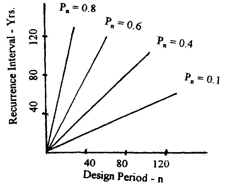
3.12 Pn = (1 – 1/Tr)n log Pn = n Log (1 – 1/Tr) n = log Pn/log (1 – 1/Tr)
A straight line can be defined by this equation and the following probability curves will appear.
Month Inflow I Draft O Deficiency O - I Cumulative Deficiency Σ (O – I)* April 97 21.8 -75.2 0 May 136 21.8 -114.2 0 June 59 21.8 37.2 0 July 14 21.8 7.8 7.8 Aug 6 21.8 15.8 23.6 Sep 5 21.8 16.8 40.43 Oct 3 21.8 18.8 59.2 Nov 7 21.8 14.8 74 Dec 19 21.8 2.8 76.8 Jan 13 21.8 8.8 85.6 Feb 74 21.8 -52.2 33.4* March 96 21.8 -74.2 0 April 37 21.8 -15.2 0 May 63 21.8 -41.2 0 June 49 21.8 -27.2 0

3.1320 month flow equals the sum of 12 + 11 + 10 + 12 + … + 6 + 7 + 9 = 169 cfs 3.14 3.15
3.16 Reservoir capacity = 750 acre-feet
Reservoir yield is the amount of water which can be supplied during a specified time period. Assume the reservoir is to be operated continuously for 1 year without recharge. Also assume that evaporation, seepage, and other losses are zero.
Max continuous yield is 750 acre-ft/year
Or 750 X 43,560 X 0.304 = 917, 846 cubic meters per year
Or 750 X 43,560 X 7.48 X 365 X 24 X 60 = 465 gpm continuously for 1 year
3.17 Constant annual yield = 1500 gpm
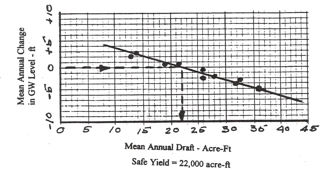
Reservoir capacity = ? Time of operation without recharge = 1 yr
Res. Capacity = 1500 X 365 X 24 X 60 X 0.134 X (1/43,560) = 2,425 ac-ft/yr
This storage will provide a yield of 1,500 gpm for one year without any recharge
3.18 mean draft = 100 mgd, catchment area = 150 sq. mi., reservoir area = 4000 acres
rainfall = 38 inches, runoff = 13 inches, evaporation = 49 inches (mean annual)
(a) gain or loss in storage = ?
ΔS = rainfall + runoff – evaporation – draft
rainfall = 38 X 4000 X (1/12) = 12,667 ac-ft
runoff = [(150 X 640) – 4000] X 13 X (1/12) = 99,967 ac-ft
evaporation = 49 X 4000 X (1/12) = 16,333 ac-ft
draft = 100,000,000 X 365 X 0.134 X (43,560) = 112,282 ac-ft
ΔS = 12,667 + 99,667 – 16,333 – 112,282 = -16,281 ac-ft
The net loss in storage is 16, 281 ac-ft
(b) volume of water evaporated = 16,333 ac-ft
given a community of 100,000 people, assume a consumption of 150 gpcd
water demand = 100,000 X 150 X 365 = 5,475 mg/year
volume evaporated = 16,333 X 43,560 X 7.48 = 5,304 mg/year evaporated water could supply the community with their water needs for 5304/5475 = 0.97 or for about one year
3.19 Use equation 3.29
K = 0.000287
h = 43
m = 8
n = 15
q = 0.000287*8*43/15 = 0.006582
Total Q is therefore 50*0.006582 = 0.325 cfs
3.20 q= 000084*8*22/15 = 0.000986
Q = 0.0007872*35 = 0.0345 m3/s
3.21
u
(1.87r2Sc)/Tt = (1.87 * 1 * 6.4 * 10-4)/(6200 * 7.5 * 24 * 60) =
x 10 -10
W(u) = 20.3
(114.6 * 60,000 * 7.5 * 20.3)/(6,200 * 7.5 * 24 * 60) = 15.6 3.22 ) ( ) / log( 528 1 2 1 2 h h m r r Q K f 2 554 1) 90*(10 528*850*log(10) ft gpd K f
) / 1055log( ) ( 1 / 2 2 1 2 2 r r h h K Q f 37107 0 100) 235 log( ) log( 1 2 r r ft h ft h 8 77 2 22 100 79 21 100 1 2 gpm Q 634.44 1055*0.37107 77.8 1320(79 2) 2 3.24
=
8.58
Interpolating,
S =
3.23
Equation 3.20 is applicable
Using Equation 3.35, u can be computed
Referring to Table 3.5 and interpolating, we estimate W(u) to be 9.1. Then using Equation 3.34, the drawdown is found to be:
3.25 (a) Using Equation 3.35, u can be computed as follows:
Then from Table 3.5, W(u) is found to be 0.36. Applying Equation 3.33, the drawdown can be determined
(c) Follow the procedure used in (a)
Then from Table 3.5, W(u) is found to be 4.06. Applying Eq. 3.33, the drawdown can be determined
3.26 (a) Using Equation 3.31, u can be computed as follows:
0
Then from Table 3.5, the drawdown can be determined,
(b) Follow the procedure used in (a)
5 4 4 2 23*10 6 *12 3*10 *3*10 1.87*200 u
ft s 41 10 3*10 114.6*9.1*300 4
71 0 0028 4*1000*0 90*90*0.00098 u
m s 0.039 *0.0028 4* 0.0038*0.36
0098
4*72000*0
u
0 0028
90*90*0.00098
m s 0.44 *0.000028 4* 0.0038*4.06
25
4*3600*0.0028
u
m s 0.12 *0.0028 4* 0.004*1.07
100*100*0.001
0.01 4*24*60*60*0.0028
u
100*100*0.001
Then from Table 3.5, W(u) is found to be 4.04 Applying Equation 3.33, the drawdown can be determined
3.27 (a) Using Equation 3.31, u can be computed as follows:
Then from Table 3.5, the drawdown can be determined,
(b) Follow the procedure used in (a)
Then from Table 3.5, W(u) is found to be 3.24 Applying Equation 3.33, the drawdown can be determined
m s 46 0 0028 *0 4* 04 004*4 0
0.46 0028 4*12*60*60*0 001
u
m s 05 0 *0.0028
0.003*0.36
150*150*0
4*
023 0 0028
500*500*0.001 u
4*12*60*60*0
m s 28 0 0028 *0 4* 24 003*3 0 3.28 13,392 (120/45) 528*log 600*2*3.1416*100*8 (120/45) 528*log ) *( *2* 10 10 1 2 h h K Q f gal/min 3.29 407.62 100*1.28 (500/75) 528*1200*log ) ( ) / ( *log 528* 10 1 2 1 2 10 h h m r r Q K f gpd/ft2 3.30 h Q T 264* From a plot of drawdown versus t, drawdown per log cycle is 28.2 – 10.5 = 17.1 *17.1 264 T Q Converting T to gal/day/ft T=5100 330 *17.1 264 5100 Q gpm
3.31 From plot of data, t0=1.25 minutes = 20.87 x 10⁻³ ft/day, and from plot,
3.35 Use Equation 3.37 and refer to figure which follows
Dh 14 feet 5657 14 264*300 T gpd/ft 0.00041 60 0.3*5657*0.87*10 * 0.3* 2 3 2 0 r t T S c 3.32 0.00011 * 1.87* 2 Tt S r u c W(u)=-0.577216-ln(u) Substituting and solving, using loge(u) W(u)=8.537 8.84 3.1*10 114.6*280*8.537 ) ( * 114.6* 4 T u W Q S feet 3.33 Use Equation 3.22 477 0 ) ln( 1 2 r r 13,468 528*0.477 *100*9 600*2* Q gpm 3.34 Use Equation 3.23 2 433.2 130*10.8 ) 65 500 528*1300*ln( ft gpd K f
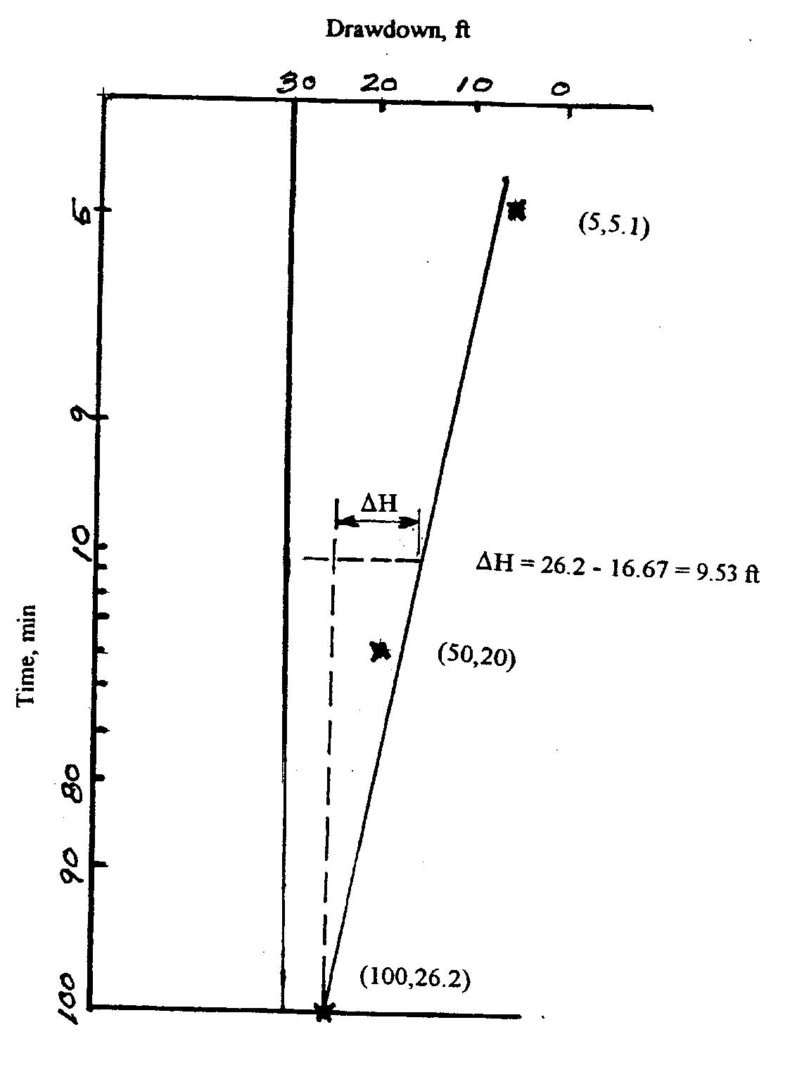 T=700*7.5 = 5250 gpd/ft
5 189 264 5250*9.53 Q gpm
From Fig change in head is 9.53 feet
Use Equation 3.19
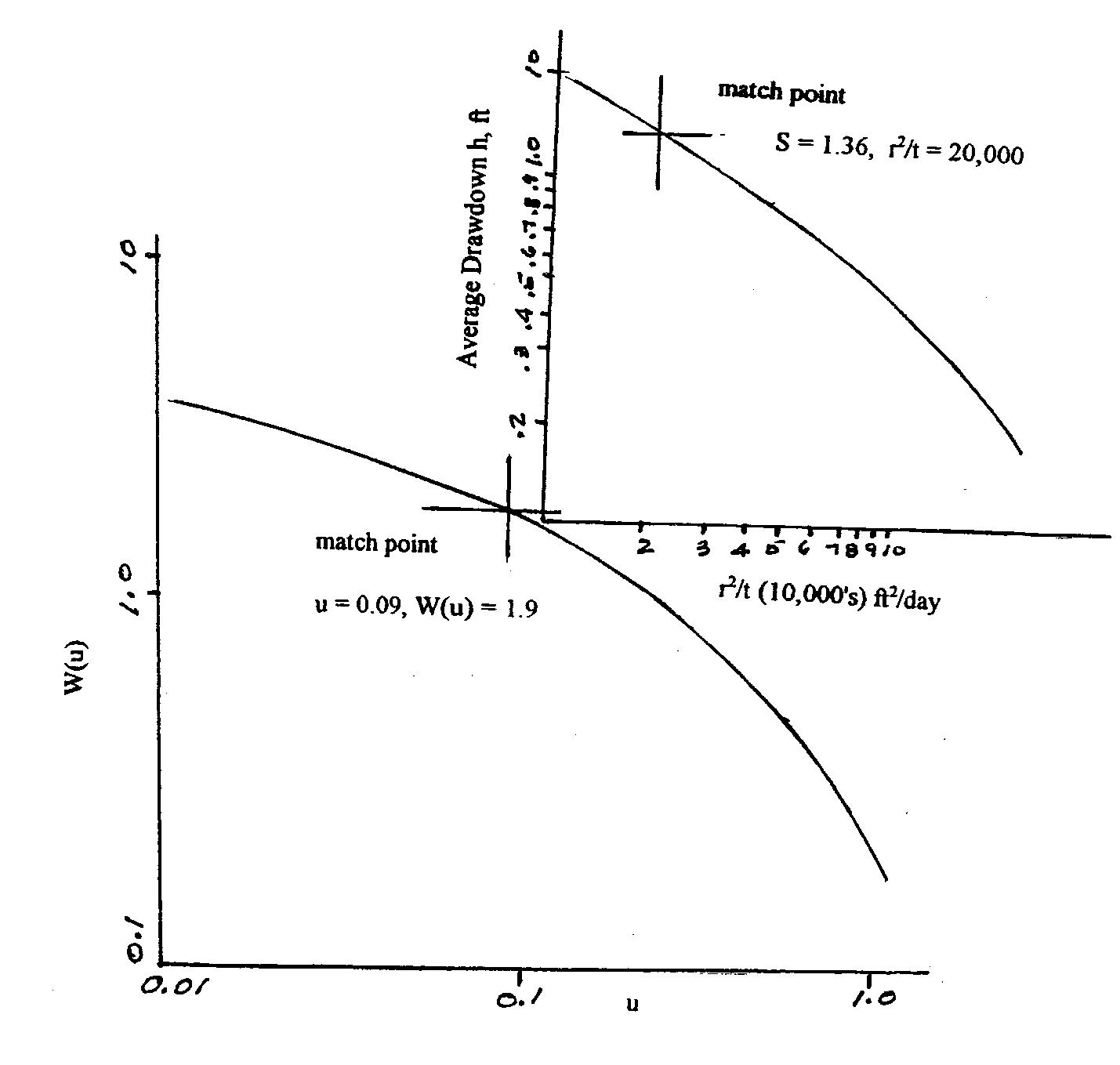
3.37 Use Equations 3.34 and 3.35 refer to the following figure determine s and r2/t from the figure = 1.36 and 20,000
from the figure = 0.09 and 1.9
3.36
41683 0 ) ( log 1 2 10 r r Q= 881 41683 1055*0 77.5*77.5) 1300*(79.4*79.4 gpm
Determine u
W(u)
ft gpd T 80,050 365 1 114.6*500*1.9 1926 0 87*20000 1 09*80050 0 c S
and

3.38 Use Equation 3.19 2 1 2 2 2 100 ) 60 (100 66 50 y 1560 2 1 y , y1=39.5 Drawdown is 100-39.5=60.5 feet 3.39 Use Equation 3.23 Log of the ratio = 0.1856 2 8 428 95) 80*(97 528*700*0.1856 ft gpd K f Water Supply and Pollution Control 8th Edition Viessman Solutions Manual Full Download: http://testbanktip.com/download/water-supply-and-pollution-control-8th-edition-viessman-solutions-manual/ Download all pages and all chapters at: TestBankTip.com


 T=700*7.5 = 5250 gpd/ft
