The Effect of Crime Rates on Housing Prices: A Hedonic Study, John Paul Goncalves

The Effect of Crime Rates on Home Prices:

A Hedonic Study

John Paul Goncalves1

Abstract:

The hedonic regression model in this study is from a Florida based study that has been applied on a national level. The results of this research will indicate the most significant variables which support the overall effect on the price of a home. The emphasis of this study is to examine the overall impact of crime rates on average home prices in America’s state capitals.

JEL Classification: R21, R22

Keywords: crime rates, home price, state capitals

1 Department of Economics, Bryant University, 1150 Douglas Pike, Smithfield, RI 02917. Phone: (401) 578-4307. Email: jgoncal1@bryant.edu

1.0 Introduction

Crime is a challenge populations have faced since the creation of the first villages in this world. Basic theory shows that villages, towns, or cities that have minor or no existent form of laws or punishment system will experience more crime than pockets that have introduced these safety measures. The United States of America, a very civilized high income country, has sought for low crime. With the investment of trillions of dollars into introducing and creating police academies, barracks, law enforcement systems, judicial systems, and other precautionary investments, safety and lower crime rates should be ensured. Yet, only in the year 2005 did the US experience a decrease in its total crime rates. Considering these ‘precautionary investments’ have been in place since the US won its independence it is easy to state that the system is inefficient and that marginal costs greatly outweigh the marginal benefits. Should America worry about this inefficiency when crime rates have been diminishing?

Yes, the US should be concerned. Why? Well, as known, the US and the rest of the world are currently experiencing recessionary-like shocks. Furthermore, historically, crime wanes during periods of economic growth and surges during economic downturns.1 Therefore, many cities across the US are possibly on the verge of a major crime wave. How legitimate is this historical fact? As economists, academics, criminologists, and demographers argue, crime is caused by the economy, unemployment, racism, and poverty.2 For that reason the likelihood of a crime wave occurring in the US is plausible.

A crime wave is of course unsafe and problematic for the public, but at the same time very costly. For years, police chiefs have argued that safer cities are better for business, increase tax revenue and help property values. Consequently, if crime increases, state capitals must cope with deteriorating communities which lower property value, which then lower the amount of tax revenue and new business creation. For instance, James Larsen, a professor at Wright State University, found that home sales prices located within one-tenth a mile of a sex offender

1 Gabriel Kahn, “Top Cops in Los Angeles says cutting crime pays.” WSJ, November 29, 2009 2 Gabriel Kahn, “Top Cops in Los Angeles says cutting crime pays.” WSJ, November 29, 2009

dropped 17% in value.3 Moreover, due to US crime rates, it is expected that property values across the country will decline $1.2 trillion in 2008.4

All in all, the justification that, an increase in crime rates will decrease property values can be made. Hence, Hellman and Naroff’s (1979) and Rizzo’s (1979) verification that crime has a trivial impact on home prices is also true. For these reasons, this study should similarly resemble the facts established above, and the previous results of researchers like Hellman, Naroff, and Rizzo.

Additionally, this national level study will introduce a first look into the determinants of house prices using weighted variables such as cost of crime indexes. The structure of this study is as follows. Section two introduces crime trends in the US. Section three introduces the idea

behind cost of crime and its imperative purpose in this study. A literature review follows in section four to help support the overall idea and methodology. Section’s five and six establishes the data, empirical methodology, results to the empirical methodology, and an analysis on the results. The remaining sections include: implications with the study, and concluding remarks.

2.0 Crime Trends

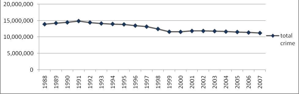
Figure 1

This figure shows total reported crimes, both violent and property, in the U.S. Total crime has diminished in the long run, but has remained steady in recent years. Source: FBI Crime in United States (CIUS) index (2008)

3 Lisa Scherzer, “Three Home Value drains to Avoid.” WSJ, June 16, 2008 4 Emily Frielander, “Cities dealing with rise in abandoned properties.” WSJ, January 28, 2008

Figure 2

This figure shows the total reported crime and the average property value of single family dwellings in U.S. state capitals. Even though crime has diminshed in the long run, as shown in figure 1, it still does have an effect on the average house price. Source: Census Bureau, FBI CIUS index, and Trulia.com (2008)

Figure 3

This figure breaksdown the total reported crime rate in each geographical region of the U.S.

Source: FBI CIUS index (2008)

3.0 The Cost of Crime

Normal crime indexes create an equilibrium that does not exist. A weighted index using the cost of crime will remove this equilibrium. Normally, when police are comparing public safety across jurisdictions, the total number of offences reported in a jurisdiction will be divided by the population of that jurisdiction. But how does this public safety figure truly measure the differences of safety between jurisdictions? For instance, in 2007, town A, with a population of a 1000, reported 100 murders while town B, with a similar population, reported 100 burglaries. In the end, both towns have a crime index of .1 or 10% (100 murders or burglaries/1000 population). How is this index an accurate assessment of public safety differences when burglaries and murders are proportionate?

Luckily, this problem is simple to fix. By weighting the index through the figures from Cohen et al. (1995), the true implicit costs will be recognized and the bias in which murders and burglaries are equal will be removed.

Town Population Reported Offences Normal Crime Index Cohen cost index New Index level

A 1000 100 murders .1 or 10% $2,740,000/murder $274,000,000

B 1000 100 burglaries .1 or 10% $1,500/burglary $150,000

After applying the Cohen et al. index to the earlier example, the equilibrium between the two towns is dramatically altered. Due to the fact that Cohen et al. found murders to obtain a more significant impact on victims than a burglary, town A now appears to be a hazardous jurisdiction compared to town B.

Allen and Rasmussen’s (2001) study found similar results. By ranking cities by Cohen et al. (1995) index rather than the traditional index crime, Tallahassee’s metropolitan area improved from 5th in the nation to 54th and New York diminished from 73rd to 7th. Overall, this example clarifies the significance and reliability of Cohen et al. index. On the other hand, many

economists and psychologists question this reliability. Butterfield (1996) criticizes the method behind the victim cost estimates because determining psychic costs seems impossible.

Once again, the Cohen et al. victimization cost index will be used in the analysis of how crime effects house prices in America’s state capitals. The index will weigh the crimes in which the FBI has documented as reported in the year of 2008 in these state capitals. Although this paper does adopt this cost index as a more reasonable and preferred method of measure, it does not necessarily accept the authenticity of these specific estimates.

4.0 Literature Review

Hedonic modeling breaks-down the dependent variable being studied into its essential characteristics, and then estimates values for each of these characteristics. This style of regression is very popular in real estate economics. Due to the fact that buildings are a heterogeneous good, the hedonic model approach focuses on the buildings characteristics, such as bedrooms, and lot size for a better interpretation of the total value or price of a building. Cohen (1995) and Rasmussen (1990) dispute that hedonic studies of housing markets show that the value of spatial differences in education, air pollution, property taxes, and other location specific attributes will be capitalized into house prices.

Allen and Rasmussen (2001) created a hedonic model to measure the effect crime has on the average home price. This study was focused on the Jacksonville, Florida area, and included 2880 observations. With this size observation and the in-depth hedonic model, which has assistance from Cohen et al. crime index to create some weighted variables, Allen and Rasmussen were able to prove crime has a significantly negative effect on home prices in the Jacksonville area. Therefore showing the true importance a weighted crime index has in hedonic studies. This data source led to the creation of the hedonic model which is being used in this empirical study.

Thaler (1978) approximated the impact property crime in Rochester, NY had on nearby home prices by using a cost of crime and implicit price model. Cohen (1990) concurs by stating it is necessary with hedonic models to use the cost of crime rather than index crime data to estimate the effect on home prices.

Hellman and Naroff (1979) and Gibbons (2004) conducted studies to find the impact crime had on urban communities and property values. Overall, the two studies cause similar effects.

For instance, Hellman and Naroff believe crime does cause variations in home prices which then reduce property tax revenue for communities. Meanwhile, Gibbons suggests the direct costs associated with property crime may discourage home-buyers, inhibit local regeneration and catalyses a downward spiral in neighborhood status; basically this lowers demand, in which lowers prices. All in all, deterioration from crime in urban communities leads to downward pressure on home prices.

This study adds onto to the overall research started by Allen and Rasmussen by applying it to a national level. Most hedonic modeled studies on crime and real estate property values are based in one city or district. Unfortunately most urbanized large cities (which are the most commonly used) have higher crime rates than the millions of towns in America; therefore the ‘value’ found in Allen and Rasmussen’s can never be used to report the deterioration crime has on property values nationwide. This national level study will remove that bias and create a more consistent ‘value’ for the many towns in America.

5.0 Data and Empirical Methodology

The data for this study comes from various sources. The Census Bureau provided data on average house prices for each of the fifty capitals in the United States in 2008. These average prices were then used to search homes that sold at that average price between January 1, 2008 and December 31, 2008 on Trulia.com. The remaining data points are placed under three different categories in the Hedonic model:

Where:

Pi = the selling price of the home Si = a vector of housing and lot characteristics Ni = a vector of neighborhood characteristics Ci = the number of crimes and the estimated cost of the number of crimes

Ten homes were picked from each capital, and then averages of each characteristic of the ten homes were created into variables. These independent variables are sited under the housing and lot characteristics (Si). The variables are as follows: number of bedrooms and bathrooms;

Pi = f (Si, Ni, Ci)

square footage of home and lot; age of home in years; and dummy variables for pool, fireplace, central air, fenced yard, gated community, and waterfront property. Zietz and Sirmans’ (2008) quantile regression on determinants of house prices supports these independent variables. For example, variables such as square footage, lot size, bathrooms, and floor type impact selling price, while other variables have a relatively constant effect on selling price. For better understanding please refer to table 2 and 3. Neighborhood characteristics were provided by the Census Bureau and Federal Bureau of Investigation (FBI). The independent variables under this vector include: population for each capital; percentage of population that is Caucasian, African American, and Hispanic; the proportion of population that is either “17 & under,” “18-24,” or “55 & over;” and the median income in each capital. Overall, this creates a total of eight independent variables for “Ni”. The reasoning behind creating three variables for age is because certain age groups commit more crimes than others. As Lynch and Rasmussen (2001) found in their study, the population between 18 and 24 years old is the most crime prone portion in the United States. Therefore it is expected that this group has a significantly negative effect on home prices. Furthermore, the median income level is expected to have a positively significant affect on home prices as the level increases. Income and personal property investment are believed to be positively related. Thus, if median income increases then investment increases, which improves the appraisal and sale price of a home. For better understanding please refer to table 2 and 3. The FBI provided the index of data on crime rates for each capital. The index consisted of counts on violent crimes (manslaughter/murder, forcible rape, robbery, aggravated assault) and property crimes (burglary, larceny-theft, motor-vehicle theft, arson). Questions might arise on why variables such as motor-vehicle theft were used when analyzing house prices. Well, home prices are not only valued through appraisals, structural components, and sale prices, but also through the laws of supply and demand. For instance, if a city has a 70% motor-vehicle theft possibility, no matter how well a home fits a buyer’s necessities, demand will decrease due to the greater chance of having their car stolen. As demand decreases the price of homes in the city will follow. That is why, when accounting for crime rates all forms must be taken into consideration.

Moreover, Cohen et al. 1995 study provides the approximated cost for each form of crime listed above. The costs were then administered to the count of crimes each city experienced.

This formed the weighted index which will also be used during the regression. As stated earlier, by using a weighted index it removes the bias a normal counted index creates. It is expected that the weighted index will be negatively related to home prices (i.e. higher cost of crime leads to lower home prices). For better understanding please refer to table 2 and 3.

6.0 Empirical Results and Analysis

Table 1 reports the results from the hedonic regression model. The table includes two regressions; both of which are indistinguishable besides the removal of a fenced yard and gated community dummy, addition of percentage of population 18-24, and most importantly the removal of reported crime variables. The fenced yard and gated community variables were removed due to high triviality. The raw data hardly included any observations with these options. As shown in table 1, both variables have a negative effect on house prices. This is obviously false. As Allen and Rasmussen (2001) found in their study, fenced yards and gated communities are valued more in a high crime area because these attributes represent a barrier between the house and the street. Meaning, consumers are willing to pay a higher price for a home including these attributes, not pay lower. If the observations, included in this study, had a proper mix of fenced, non-fenced, gated community, and non-gated community properties, rather than strictly non-fenced and nongated communities, then the two variables would have been more effective. Overall, the variables were removed for regression 2. Differing from these variables is the percentage of population 18-24 years of age variable. As stated earlier, this was added onto regression 2 because Allen and Rasmussen’s study, along with reliable news sources, provided facts supporting that this age bracket commits the highest amount of crime in the United States. Therefore, it would be expected that 18 to 24 year olds would have a negative effect on house prices. Furthermore, table 2 supports the negative relationship. In fact, this age bracket reduces house prices by 1.44%. On a side note, as revealed in table 1, the independent variables that affect house prices in a statistically significant manner (meaning the 1%, 5% and 10% significance levels) in regression 1 are size of home (sq ft), age of home, central air, waterfront property, population, and median income. Little change occurred in regression 2; the statistically significant variables that affect house price are size of home (sq ft), lot size, age of home, pool, waterfront property, population, percentage of population that is Caucasian, and median income. Unfortunately, the weighted cost

of crime variables were not found to be significant at either the 1%, 5%, or 10% levels, but the expected relationship to the dependent variable was proven true. As table 3 reflects, the two weighted crime index variables (property and violent) are expected to have a negative effect on house prices. Table 1 reports that property crime has a 3.99% or $8,841 depreciation on home values in these state capitals5; meanwhile, violent crime has a 2.67% or $5,916 depreciation on home values in the same state capitals. The outcomes of the expected relationship to the dependent variable are identical with Allen and Rasmussen’s study, but the ‘value’ from the regression output differs. They found property crime would decrease property values by $206 and violent crimes to reduce it by $145. Why such a noteworthy difference? Perhaps, due to Allen and Rasmussen (2001) focus on single family homes in the Tallahassee area, their mean home price is at a lower value due to observations sharing similar traits and buyer patterns. There mean level house value is $95,532 and this study’s is $221,592. At the national level, the observations are exposed to different characteristics that affect their appraisal value and sale price; such characteristics are home features, land and property values, buyer patterns and demand. In addition, by this study having a higher mean level, the percentage affect the weighted crime indexes have on home values is larger. On an end note, these two dollar ‘values,’ are superior estimates which may be interchangeably used on any home in America.

7.0 Implications with Study

Alas, the two costs of crime weighted variables were not found to be significant in the regression output. It is believed that the low sample size and high amount of independent variables produced a problem with the degrees of freedom. All in all, significance was not apparent in many variables, two of which being the variables with the outright highest importance to the study. Even though the two variables did not show significance at the 1%, 5% or 10% level, they did have the predicted negative relationship to the dependent variable. As stated earlier, this can all be found in table 1 and table 3.

Nonetheless, even with the variables not being significant, there is still enough evidence and support from other previous studies to support the outcome. Thaler (1978), Taylor (1995), Rizzo (1979), Lynch and Rasmussen (2001), and Rasmussen and Zuehlke (1990) all have found crime

5 The 3.99% taken from table 1 is applied to the mean selling price of home variable in table 4

to have a negative impact on the average house price within a surrounding area; majority of the time the surrounding area has been a large city, just as this study is based on sizeable state capitals.

8.0 Conclusion

In more recent times, the value of homes has been decreasing due to economic factors, never mind the many other external factors such as crime. Therefore if homeowners live in an area with high crime they have much at stake. In fact, with the use of macro-level data, this study finds that homes values can experience negative affects as high as $8,841 due to crime. A deplorable figure that could diminish appraisal levels, supply markets and/or demand markets of towns, states, or nations.

Though this study provides several appealing results, this analysis was only for US state capitals, and it is possible the same results will not apply to other cities and towns nationwide or in other countries. This study could be replicated or manipulated to fit the needs of other future studies for similar hedonic studies, or weighted cost of crime analysis.

References

Butterfield, F. (1996) Prison: where the money is, New York Times, 2 June, p. 16.

Cohen, M. A., T. R. Miller, and B. Wiersema. “Crime in the United States: Victim Costs and Consequences.” Final Report to the National Institute of Justice, 1995

Emily Friedlander, “Cities dealing with rise in abandoned properties.” WSJ, January 28, 2008

Gabriel Kahn, “Top Cops in Los Angeles says cutting crime pays” WSJ, November 29, 2008

Gibbons, Steve. “The Cost of Urban Property Crime.” The Economic Journal v. 114 22pp Nov. 2004

Hellman, Daryl and Joel Naroff. “The Impact of Crime on Urban Residential Property Values.” Urban Studies v. 16 7pp Feb. 1979

Lisa Scherzer, “Three Home Value drains to Avoid, WSJ, June 16, 2008

Lynch, Allen and David W. Rasmussen. “Measuring the Impact of Crime on house prices.” Applied Economics v. 33 1981-1989 Nov. 2001

Peek, Joe and James A. Wilcox. “The Measurements and Determinants of Single-Family House Prices.” AREUEA Journal vol. 19 31pp Nov. 1991

Rasmussen, D. W. and T. W. Zuehlke. “On the Choice of Functional Form for Hedonic Price Functions.” Applied Economics vol. 22 431-438 Mar. 1990

Rizzo, M. J. “The Cost of Crime to Victims: an Empirical Analysis.” Journal of Legal Studied vol. 8, 177-205 1979

Taylor, Ralph. “The Impact of Crime on Communities.” Annals of the American Academy of Political and Social Science vol.539 17pp. May 1995

Thaler, R. “A note on the Value of Crime Control: Evidence from the Property Market.” Journal of Urban Economics vol. 5 137-145 1978

Zietz, Joachim, E. M. Zietz and G. Sirmans. “Determinants of House Prices: A quantile regression approach.” The Journal of Real Estate Finance and Economics vol.37 317-333 Nov 2008

All data sources are from the: Census Bureau, Federal Bureau of Investigation, and Trulia’s Real Estate website Table 1: Regression Results

Variable

Size of home(sq ft) Lot Size (sq ft) Bedrooms

Regression 1 Regression 2

0.0000781** 0.0000985*** 0.00000152 0.00000204* 0.008838 -0.008507

Bathrooms -0.057953 -0.034343

Log(age of home) Pool (dummy) 0.133269*** 0.120889*** -0.067385 -0.09712**

Fenced Yard (dummy) -0.033424 Gated Community (dummy) -0.01392 Fireplace (dummy) 0.03597

0.04659 Central air (dummy) 0.077085* 0.05958

Waterfront property (dummy) 0.234036** 0.191848** Population 0.000000205** 0.000000194**

Percentage of Pop. Caucasian -0.001957 -0.003858** Percentage of Pop. African American -0.000522 -0.000421

Percentage of Pop. Hispanic 0.004305 0.005799

Percentage of Pop. 17 & under -0.001493 -0.00394 Percentage of Pop. 18-24 -0.014468

Percentage of Pop. 55 & over -0.003971 0.000999 Median Income 0.0000124*** -0.0000130*** Log(property crime) 0.026386 Log(violent crime) -0.150789

Log(cost of property crime) -0.036795 -0.039917

Log(cost of violent crime) 0.087093 -0.026689 Adjusted R-Squared 0.810289 0.816403 F-Statistic 9.542349 11.76572

Note: ***, **, and * denotes significance at 1%, 5%, and 10%

Table 2: Variable Definition

Variable

Size of home (Sq. ft)

Lot Size (Sq. ft)

Bedrooms

Definition

The square footage of living area

The square footage of the lot the home is built on

Number of bedrooms in the home

Bathrooms Number of bathrooms in the home

Log Age of Home The log of the age of home in years

Pool (dummy)

Fenced Yard (dummy) Whether or not the home has a pool

Whether or not the home has a fenced yard

Gated Community (dummy) Whether or not the home is in a gated community

Fireplace (dummy) Whether or not the home has a fireplace

Central air (dummy) Whether or not the home has a central air cooling system

Waterfront Property (dummy) Whether or not the home is a waterfront property

Population Total population of the state capital

Percentage of Pop. Caucasian Percentage of population in state capital that is Caucasian

Percentage of Pop. African American Percentage of population in state capital that is African American

Percentage of Pop. Hispanic Percentage of population in state capital that is Hispanic

Percentage of Pop. 17 & under Percentage of population in state capital that is 17 & under

Percentage of Pop. 18-24 Percentage of population in state capital that is 18-24

Percentage of Pop. 55 & over Percentage of population in state capital that is 55 & over

Median Income The median income of the population in the state capital

Log of Total Property Crime Total reported property crimes in state capital

Log of Total Violent Crime Total reported violent crimes in state capital

Log of Total Cost of Property Crime1 Total cost of reported property crimes in state capital

Log of Total Cost of Violent Crime1 Total cost of reported violent crimes in state capital

1 measured accordingly with Cohen et al. cost of crime index

Table 3: Expected Sign Chart

Variable

Size of home(sq ft)

Lot Size (sq ft)

Bedrooms

Bathrooms

Log(age of home)

Pool

Fenced Yard

Gated Community

Fireplace

Central air

Waterfront property

Population

Percentage of Pop. Caucasian

Percentage of Pop. African American

Percentage of Pop. Hispanic

Percentage of Pop. 17 & under

Percentage of Pop. 18-24

Percentage of Pop. 55 & over

Log(property crime)

DataSource Expected

Trulia.com

Trulia.com

Trulia.com

Trulia.com

Trulia.com

Trulia.com

Trulia.com

Trulia.com

Trulia.com

Trulia.com

Trulia.com

FBI

Census Bureau

Census Bureau

Census Bureau

Census Bureau

Census Bureau

Census Bureau

FBI

Log(violent crime) FBI (-)

Log(cost of property crime) FBI/National Institute of Justice (-)

Log(cost of violent crime) FBI/National Institute of Justice (-)

Table 4: Mean and Standard Deviation of variables used in housing market analysis

Variable

Selling Price of Home1 Log Selling Price of Home Size of Home (Sq ft) Lot Size (Sq ft) Bedrooms Bathrooms Log Age of Home Pool (dummy) Fireplace (dummy) Central Air (dummy) Waterfront Property (dummy) Population Percentage of Pop. Caucasian Percentage of Pop. Hispanic Percentage of Pop. African American Percentage of Pop. 17 & under Percentage of Pop. 18-24 Percentage of Pop. 55 & over Median Income1 Total Property Crime1 Total Violent Crime1 Total Cost of Property Crime1 Total Cost of Violent Crime1 1measured in US currency ($)

Mean Standard Deviation

221592 104123.926 5.307472 0.177271

1799.447 524.4969

12646.38 3.0212766

13967.96 0.6075382 2.11702128 0.56349806 1.367905 0.276596 0.638298 0.467091 0.452151 0.485688

0.489362 0.042553 274320.04 .7830426 0.505291 0.20403 304173.92 .1480769

.02810638 .1167447 .2770851 .0268249 .1211297 .03438202

.1418936 .2125106 50381.42 .01357305 .02728981 7602.874

14853

17667.237 2429 2839.436598 20,547,932 27,613,128 134,140,043 171,033,669

Table 5: Determinants of House Prices

Variables Coefficient Std. Error t-Statistic Prob.

Size of Home (Sq. ft) Lot Size (Sq. ft) Bedrooms Bathrooms 0.0000781 0.0000364 2.142413 0.043 0.00000152 0.00000119 1.272231 0.216 0.008838 0.040737 0.21695 0.8302

-0.057953 0.036739 -1.577432 0.1284

Log Age of Home Pool (dummy) Fenced Yard (dummy) Fireplace (dummy) Central Air (dummy)

0.133269 -0.067385 -0.033424 0.03597 0.077085 Waterfront Property (dummy) 0.234036 Gated Community (dummy) -0.01392 Population 2.05E-07 0.040489 3.291462 0.0032 0.041861 -1.609722 0.1211 0.031623 -1.056954 0.3015 0.030181 1.191839 0.2455 0.041373 1.863179 0.0753 0.089741 2.60791 0.0157 0.052839 -0.263448 0.7946 8.75E-08 2.346569 0.0279

Percentage of Pop. Caucasian -0.001957 Percentage of Pop. Hispanic 0.004305 Percentage of Pop. African American -0.000522 Percentage of Pop. 17 & under -0.001493 0.002303 -0.850056 0.4041 0.006936 0.620775 0.5409 0.002281 -0.22874 0.8211 0.005004 -0.298429 0.7681

Percentage of Pop. 55 & over -0.003971

0.006093 -0.651732 0.521 Median Income 0.0000124 0.00000237 5.239734 0 Log Total Property Crime 0.026386 0.188645 0.139874 0.89 Log Total Violent Crime -0.150789 0.102065 -1.477377 0.1531 Log Total Cost of Violent Crime 0.087093 0.098738 0.882059 0.3869 Log Total Cost of Property Crime -0.036795 0.177647 -0.207127 0.8377 Constant 4.888821 0.630297 7.756372 0

R-squared Adjusted R-squared S.E. of regression Sum squared resid Log likelihood F-statistic Prob(F-statistic) 0.905144 Mean dependent var 0.810289 S.D. dependent var 0.077212 Akaike info criterion 0.137119 Schwarz criterion 70.48065 Hannan-Quinn criter. 9.542349 Durbin-Watson stat 0 5.307472 0.177271 -1.9779 1.033144 1.622382 2.020402

Table 6: Determinants of House Prices using Weighted Index

Variables Coefficient Std. Error t-Statistic Prob.

Size of Home (Sq. ft) Lot Size (Sq. ft) Bedrooms Bathrooms 9.85E-05 3.35E-05 2.938795 0.0067 2.04E-06 1.15E-06 1.766758 0.0886 -0.008507 0.035681 0.238418 0.8134 -0.034343 0.035055 0.979691 0.3359

Log Age of Home Pool (dummy) Fireplace (dummy)

0.120889 0.036856 3.280007 0.0029 -0.09712 0.035826 2.710893 0.0115 0.04659 0.028197 1.652292 0.1101 Central Air (dummy) 0.05958 0.038029 1.566687 0.1288 Waterfront Property (dummy) 0.191848 0.084128 2.28043 0.0307 Population 1.94E-07 8.30E-08 2.34314 0.0267 Percentage of Pop. Caucasian -0.003858 0.001841 2.096232 0.0456 Percentage of Pop. Hispanic 0.005799 0.006618 0.876229 0.3886 Percentage of Pop. African American -0.000421 0.002227 -0.18912 0.8514 Percentage of Pop. 17 & under -0.00394 0.004683 -0.8414 0.4075 Percentage of Pop. 18-24 -0.014468 0.012028 1.202889 0.2395 Percentage of Pop. 55 & over 0.000999 0.006535 0.152915 0.8796 Median Income 1.30E-05 2.47E-06 5.253894 0 Log Total Cost of Violent Crime* -0.039917 0.072296 0.552138 0.5854 Log Total Cost of Property Crime* -0.026689 0.091495 0.291703 0.7727 Constant 4.955803 0.492373 10.06515 0

R-squared Adjusted R-squared S.E. of regression Sum squared resid Log likelihood F-statistic Prob(F-statistic) 0.892237 Mean dependent var 5.307472 0.816403 S.D. dependent var 0.177271 0.075958 Akaike info criterion 2.020529 0.155778 Schwarz criterion 1.233232 67.48243 Hannan-Quinn criter. 1.724264 11.76572 Durbin-Watson stat 2.052425

0

Note:* signifies Cohen et al. Cost of Crime Index