Creating Pivot Tables

After cleaning the data, PIVOT TABLES can already be created. This is the most difficult yet exciting part of data management and analysis. Go back to the indicators you selected for data analysis based on the themes you identified earlier on page 31. Focus on these indicators. Do the following steps in both worksheets.

Creating Pivot Tables

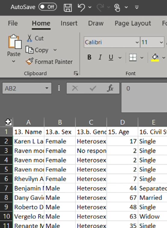
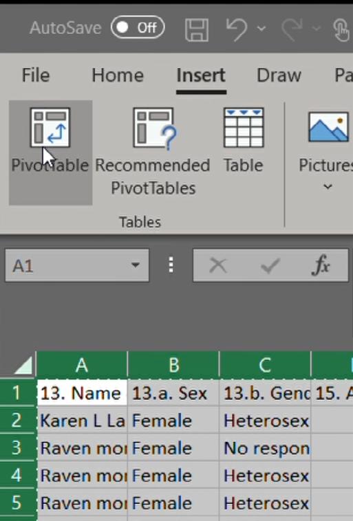
1. On the left side of COLUMN A is the SELECT ALL button. Click it to select the entire sheet. 2. Go to the INSERT MENU and select PIVOT TABLE. In other versions of

Excel it is in ‘Summarize with Pivot Table’ on the DATA TAB. 3. An option will appear to create a new spreadsheet for the Pivot Table.

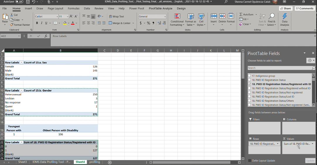
Click OK. 4. In the new sheet, HEADERS from the selected spreadsheet will appear on the right side of the screen. These are, basically, the indicators/ data gathered from IDMS. 5. HEADERS can be double-clicked or dragged into the FILTERS,

COLUMNS, ROWS, and VALUES boxes to view and display IDMS data collection results. Try putting more than one HEADERS or INDICATORS. 6. See also different examples of PIVOT TABLES that can be generated.

Using the Pivot Table, one can easily make simple summaries from the many Pivot Table Fields available in the IDMS Data. Just follow these steps: 1. Duplicate a pivot table, by selecting the entire cells it covers.

2. Copy and paste it in blank cells below the copied table. 3. Select the new Pivot Table. The PIVOT

TABLE FIELD should reappear on the right side of the screen. 4. Easily add or modify the indicators of a given Pivot Table by dragging, deleting, and manipulating the data on the Filters,

Columns, Rows, and Values areas. 5. Select an indicator from the Pivot

Table Fields. Indicator selected will automatically appear in the Column field of the table

Please check out sample pivot tables and charts using the data from CDP’s first field testing of the IDMS Tool available in an Excel File included in the IDMS Resource Materials.

Tips

If you want to get the total number of respondents of a specific indicator, select it from the Pivot Table Fields and put it in the Values box. Drag it to either the columns, rows, and values to show the data you wish to reflect on the Pivot Table. You may do this with any indicator you want to use.

To get the average value of numeric data such as age, number of persons with specific disability type, etc., put the relevant indicator/header to the values.

When you hover over any indicator and right-click, the value field settings will appear. When it appears, you can choose what value you want to summarize.