Annex II. Methodological approaches used to analyse water data

worldwide. A key advantage of compiling freshwater data using river basins (also commonly called catchments or watersheds) is that it makes it possible to present data within geographically recognized areas.

All the global and regional analysis in this report uses river basins as the common spatial denominator. Without an in-depth analysis of more local water data, there is an inherent risk of masking local areas that are experiencing a loss or degradation of freshwater ecosystems. For example, if a country has 10 river basins and nine are performing normally, with just one experiencing adverse changes, the national-level data would not identify the one degraded basin, which would be masked within the national statistic. Although national-level statistics are used for SDG reporting, there is considerable added value in providing freshwater ecosystem information to countries at the river basin level.

Aquifers, lakes and river basins shared by two or more countries account for an estimated 60 per cent of global freshwater flow and are home to more than 40 per cent of the world’s population. The need for collaboration between riparian states to address the objectives of target 6.6 is therefore crucial.

Advanced analysis is available for each of the global data sets. This allows for more detailed data to be accessed, such as particular years or months when ecosystem conditions were changing more than normal. Countries’ national statistics on subindicators (including combined surface water, permanent water, seasonal water, reservoir water, water quality, inland wetlands, and mangroves) are available online at the SDG indicator 6.6.1 Freshwater Ecosystems Explorer and can also be directly accessed on the dedicated indicator 6.6.1 website.

Analysing surface-water extent over 20 years

SDG indicator 6.6.1. was developed to measure changes in freshwater ecosystems between 2000 and 2030. Since freshwater ecosystems (including surface-water bodies) are dynamic, a long time series of annual data is needed to identify changes that depart significantly from the longer-term mean. Changes in surface-water bodies are therefore measured in five-year intervals relative to the 2000–2019 reference period and based on the annual aggregation of monthly water occurrence maps derived from a time series of Landsat data.

High-change basins were identified by calculating the percentage change of spatial extent (Δ) of permanent waters (P), seasonal waters (S) and reservoirs (R) for each hydrological basin using the formula:

Δ = ((γ-β)/β)×100

Where:

β = median value of the spatial extent for the 2000–2019 baseline period

γ = median value of the spatial extent for the 2015–2019 reporting period

The deviations were calculated for each five-year period (2000–2004, 2005–2009, 2010–2014 and 2015–2019), with their distributions then analysed to identify the cut-off points for basins lying within the nominal range of deviations compared with those considered as differing significantly from natural variability.

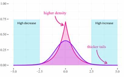
FIGURE II.1. LAPLACE AND GAUSSIAN DISTRIBUTIONS WITH EXCEEDANCE THRESHOLDS FOR BASINS WITH A HIGH INCREASE OR DECREASE IN SURFACE WATERS.

Note: Laplace distribution (red) compared with Gaussian distribution (purple). A Laplace probability density function can be applied to the deviation frequency distributions of all subindicators. The Laplace distribution is sharper at the centre and thicker at the tails compared with the better-known Gaussian distribution (Figure II.1). High-change basins for each subindicator (P, S and R) were identified by the 95 per cent confidence interval of their respective cumulative Laplace distribution functions (i.e. using the 2.5th and 97.5th percentiles as cut-off points) after adjusting for high-end outliers and excluding deserts, hyperarid basins and basins covered by permanent snow and/or ice. Although statistical anomalies, the outliers still reflect real changes, which is why they were brought back into the analysis as high-change basins despite the percentile cut-offs. Figure 0.1 depicts any basins experiencing a high change in any of the three subindicators (P, S and R), with Figures 6, 11 and 16 (and their respective sections in this report) reflecting each subindicator’s individual results, respectively.

Method for calculating changes in mangroves extent

Global mangrove area maps were generated in two phases: (i) a global map of mangrove extent for 2010; (ii) a global map of mangrove extent for 2010 with the addition of six annual data layers (1996, 2007, 2008, 2009, 2015 and 2016). Mangrove classification was limited to the use of a mangrove habitat mask, a method that uses a combination of radar (ALOS PALSAR) and optical (Landsat-5 and -7) satellite data. These were merged into optical and radar image composites covering tropical and subtropical coastlines in the Americas, Africa, Asia and Oceania. Mangrove changes were identified from measured changes in radar backscatter intensity between 2010 ALOS PALSAR data and JERS-1 SAR (1996), ALOS PALSAR (2007, 2008 and 2009) and ALOS-2 PALSAR-2 (2015 and 2016)