Full-Service Project Management: Mansi Negi/Aptara®, Inc.
Composition: Aptara®, Inc.
Printer/Binder: Courier Kendallville
Cover Printer: Lehigh/Phoenix
Color Hagerstown
Text Font: 10/12 Minion
Credits and acknowledgments borrowed from other sources and reproduced, with permission, in this textbook appear on the appropriate page within text.
Microsoft® and Windows® are registered trademarks of the Microsoft Corporation in the U.S.A. and other countries. Screen shots and icons reprinted with permission from the Microsoft Corporation. This book is not sponsored or endorsed by or affiliated with the Microsoft Corporation.
Many of the designations by manufacturers and sellers to distinguish their products are claimed as trademarks. Where those designations appear in this book, and the publisher was aware of a trademark claim, the designations have been printed in initial caps or all caps.
Library of Congress Cataloging-in-Publication Data
Mott, Robert L.
Applied fluid mechanics/Robert L. Mott, Joseph A. Untener. — Seventh edition. pages cm
Includes bibliographical references and index.
ISBN-13: 978-0-13-255892-1
ISBN-10: 0-13-255892-0
1. Fluid mechanics. I. Untener, Joseph A. II. Title.
TA357.M67 2015
620.1'06—dc23 2013026227
ISBN 10: 0-13-255892-0
ISBN 13: 978-0-13-255892-1
This page intentionally left blank
CONTENTS
Preface xi
Acknowledgments xv
1 The Nature of Fluids and the Study
of Fluid Mechanics 1
The Big Picture 1
1.1 Objectives 3
1.2 Basic Introductory Concepts 3
1.3 The International System of Units (SI) 4
1.4 The U.S. Customary System 4
1.5 Weight and Mass 5
1.6 Temperature 6
1.7 Consistent Units in an Equation 6
1.8 The Definition of Pressure 8
1.9 Compressibility 10
1.10 Density, Specific Weight, and Specific Gravity 11
1.11 Surface Tension 14
References 15
Internet Resources 15
Practice Problems 15
Computer Aided Engineering Assignments 18
2 Viscosity of Fluids 19
The Big Picture 19
2.1 Objectives 20
2.2 Dynamic Viscosity 21
2.3 Kinematic Viscosity 22
2.4 Newtonian Fluids and Non-Newtonian Fluids 23
2.5 Variation of Viscosity with Temperature 25
2.6 Viscosity Measurement 27
2.7 SAE Viscosity Grades 32
2.8 ISO Viscosity Grades 33
2.9 Hydraulic Fluids for Fluid Power Systems 33
References 34
Internet Resources 35
Practice Problems 35
Computer Aided Engineering Assignments 37
3 Pressure Measurement 38
The Big Picture 38
3.1 Objectives 39
3.2 Absolute and Gage Pressure 39
3.3 Relationship between Pressure and Elevation 40
3.4 Development of the Pressure–Elevation Relation 43
3.5 Pascal’s Paradox 45
3.6 Manometers 46
3.7 Barometers 51
3.8 Pressure Expressed as the Height of a Column of Liquid 52
3.9 Pressure Gages and Transducers 53
References 55
Internet Resources 55
Practice Problems 55
4 Forces Due to Static Fluids 63
The Big Picture 63
4.1 Objectives 65
4.2 Gases Under Pressure 65
4.3 Horizontal Flat Surfaces Under Liquids 66
4.4 Rectangular Walls 67
4.5 Submerged Plane Areas— General 69
4.6 Development of the General Procedure for Forces on Submerged Plane Areas 72
4.7 Piezometric Head 73
4.8 Distribution of Force on a Submerged Curved Surface 74
4.9 Effect of a Pressure above the Fluid Surface 78
4.10 Forces on a Curved Surface with Fluid Below It 78
4.11 Forces on Curved Surfaces with Fluid Above and Below 79
Practice Problems 80
Computer Aided Engineering Assignments 92
5 Buoyancy and Stability 93
The Big Picture 93
5.1 Objectives 94
5.2 Buoyancy 94
5.3 Buoyancy Materials 101
5.4 Stability of Completely Submerged Bodies 102
5.5 Stability of Floating Bodies 103
5.6 Degree of Stability 107
Reference 108
Internet Resources 108
Practice Problems 108
Stability Evaluation Projects 116
6 Flow of Fluids and Bernoulli’s Equation 117
The Big Picture 117
6.1 Objectives 118
6.2 Fluid Flow Rate and the Continuity Equation 118
6.3 Commercially Available Pipe and Tubing 122
6.4 Recommended Velocity of Flow in Pipe and Tubing 124
6.5 Conservation of Energy—Bernoulli’s Equation 127
6.6 Interpretation of Bernoulli’s Equation 128
6.7 Restrictions on Bernoulli’s Equation 129
6.8 Applications of Bernoulli’s Equation 129
6.9 Torricelli’s Theorem 137
6.10 Flow Due to a Falling Head 140 References 142
Internet Resources 142 Practice Problems 143
Analysis Projects Using Bernoulli’s Equation and Torricelli’s Theorem 153
7 General Energy Equation 154
The Big Picture 154
7.1 Objectives 155
7.2 Energy Losses and Additions 156
7.3 Nomenclature of Energy Losses and Additions 158
7.4 General Energy Equation 158
7.5 Power Required by Pumps 162
7.6 Power Delivered to Fluid Motors 165 Practice Problems 167
8 Reynolds Number, Laminar Flow, Turbulent Flow, and Energy Losses Due to Friction 178
The Big Picture 178
8.1 Objectives 181
8.2 Reynolds Number 181
8.3 Critical Reynolds Numbers 182
8.4 Darcy’s Equation 183
8.5 Friction Loss in Laminar Flow 183
8.6 Friction Loss in Turbulent Flow 184
8.7 Use of Software for Pipe Flow Problems 190
8.8 Equations for the Friction Factor 194
8.9 Hazen–Williams Formula for Water Flow 195
8.10 Other Forms of the Hazen–Williams Formula 196
8.11 Nomograph for Solving the Hazen–Williams Formula 196
References 198
Internet Resources 198
Practice Problems 198
Computer Aided Engineering Assignments 204
9 Velocity Profiles for Circular Sections and Flow in Noncircular Sections 205
The Big Picture 205
9.1 Objectives 206
9.2 Velocity Profiles 207
9.3 Velocity Profile for Laminar Flow 207
9.4 Velocity Profile for Turbulent Flow 209
9.5 Flow in Noncircular Sections 212
9.6 Computational Fluid Dynamics 216
References 218
Internet Resources 218
Practice Problems 218
Computer Aided Engineering Assignments 224
10 Minor Losses 225
The Big Picture 225
10.1 Objectives 227
10.2 Resistance Coefficient 227
10.3 Sudden Enlargement 228
10.4 Exit Loss 231
Gradual Enlargement 231
Sudden Contraction 233
Gradual Contraction 236
Entrance Loss 237
10.9 Resistance Coefficients for Valves and Fittings 238
10.10 Application of Standard Valves 244
10.11 Pipe Bends 246
10.12 Pressure Drop in Fluid Power Valves 248
10.13 Flow Coefficients for Valves Using CV 251
10.14 Plastic Valves 252
10.15 Using K-Factors in PIPE-FLO® Software 253
References 258
Internet Resources 258 Practice Problems 258
Computer Aided Analysis and Design Assignments 263
11 Series Pipeline Systems 264
The Big Picture 264
11.1 Objectives 265
11.2 Class I Systems 265
11.3 Spreadsheet Aid for Class I Problems 270
11.4 Class II Systems 272
11.5 Class III Systems 278
11.6 PIPE-FLO® Examples for Series Pipeline Systems 281
11.7 Pipeline Design for Structural Integrity 284
References 286
Internet Resources 286
Practice Problems 286
Computer Aided Analysis and Design Assignments 295
12 Parallel and Branching Pipeline Systems 296
The Big Picture 296
12.1 Objectives 298
12.2 Systems with Two Branches 298
12.3 Parallel Pipeline Systems and Pressure Boundaries in PIPE-FLO® 304
12.4 Systems with Three or More Branches— Networks 307
References 314
Internet Resources 314 Practice Problems 314
Computer Aided Engineering Assignments 317
13 Pump Selection and Application 318
The Big Picture 318
13.1 Objectives 319
13.2 Parameters Involved in Pump Selection 320
13.3 Types of Pumps 320
13.4 Positive-Displacement Pumps 320
13.5 Kinetic Pumps 326
13.6 Performance Data for Centrifugal Pumps 330
13.7 Affinity Laws for Centrifugal Pumps 332
13.8 Manufacturers’ Data for Centrifugal Pumps 333
13.9 Net Positive Suction Head 341
13.10 Suction Line Details 346
13.11 Discharge Line Details 346
13.12 The System Resistance Curve 347
13.13 Pump Selection and the Operating Point for the System 350
13.14 Using PIPE-FLO® for Selection of Commercially Available Pumps 352
13.15 Alternate System Operating Modes 356
13.16 Pump Type Selection and Specific Speed 361
13.17 Life Cycle Costs for Pumped Fluid Systems 363 References 364
Internet Resources 365 Practice Problems 366
Supplemental Problem (PIPE-FLO® Only) 367
Design Problems 367
Design Problem Statements 368
Comprehensive Design Problem 370
14 Open-Channel Flow 372
The Big Picture 372
14.1 Objectives 373
14.2 Classification of Open-Channel Flow 374
14.3 Hydraulic Radius and Reynolds Number in Open-Channel Flow 375
14.4 Kinds of Open-Channel Flow 375
14.5 Uniform Steady Flow in Open Channels 376
14.6 The Geometry of Typical Open Channels 380
14.7 The Most Efficient Shapes for Open Channels 382
14.8 Critical Flow and Specific Energy 382
14.9 Hydraulic Jump 384
14.10 Open-Channel Flow Measurement 386
References 390
Digital Publications 390
Internet Resources 390
Practice Problems 391
Computer Aided Engineering Assignments 394
15 Flow Measurement 395
The Big Picture 395
15.1 Objectives 396
15.2 Flowmeter Selection Factors 396
15.3 Variable-Head Meters 397
15.4 Variable-Area Meters 404
15.5 Turbine Flowmeter 404
15.6 Vortex Flowmeter 404
15.7 Magnetic Flowmeter 406
15.8 Ultrasonic Flowmeters 408
15.9 Positive-Displacement Meters 408
15.10 Mass Flow Measurement 408
15.11 Velocity Probes 410
15.12 Level Measurement 414
15.13 Computer-Based Data Acquisition and Processing 414
References 415
Internet Resources 415
Review Questions 416 Practice Problems 416
Computer Aided Engineering Assignments 417
16
Forces Due to Fluids in Motion 418
The Big Picture 418
16.1 Objectives 419
16.2 Force Equation 419
16.3 Impulse–Momentum Equation 420
16.4 Problem-Solving Method Using the Force Equations 420
16.5 Forces on Stationary Objects 421
16.6 Forces on Bends in Pipelines 423
16.7 Forces on Moving Objects 426 Practice Problems 427
17 Drag and Lift 432
The Big Picture 432
17.1 Objectives 434
17.2 Drag Force Equation 434
17.3 Pressure Drag 435
17.4 Drag Coefficient 435
17.5 Friction Drag on Spheres in Laminar Flow 441
17.6 Vehicle Drag 441
17.7 Compressibility Effects and Cavitation 443
17.8 Lift and Drag on Airfoils 443 References 445
Internet Resources 446
Practice Problems 446
18 Fans, Blowers, Compressors, and the Flow of Gases 450
The Big Picture 450
18.1 Objectives 451
18.2 Gas Flow Rates and Pressures 451
18.3 Classification of Fans, Blowers, and Compressors 452
18.4 Flow of Compressed Air and Other Gases in Pipes 456
18.5 Flow of Air and Other Gases Through Nozzles 461
References 467
Internet Resources 467
Practice Problems 468
Computer Aided Engineering Assignments 469
19 Flow of Air in Ducts 470
The Big Picture 470
19.1 Objectives 472
19.2 Energy Losses in Ducts 472
19.3 Duct Design 477
19.4 Energy Efficiency and Practical Considerations in Duct Design 483
References 484
Internet Resources 484
Practice Problems 484
Appendices 488
Appendix A Properties of Water 488
Appendix B Properties of Common Liquids 490
Appendix C Typical Properties of Petroleum Lubricating Oils 492
Appendix D Variation of Viscosity with Temperature 493
Appendix E Properties of Air 496
Appendix F Dimensions of Steel Pipe 500
Appendix G Dimensions of Steel, Copper, and Plastic Tubing 502
Appendix H Dimensions of Type K Copper Tubing 505
Appendix I Dimensions of Ductile Iron Pipe 506
Appendix J Areas of Circles 507
Appendix K Conversion Factors 509
Appendix L Properties of Areas 511
Appendix M Properties of Solids 513
Appendix N Gas Constant, Adiabatic Exponent, and Critical Pressure Ratio for Selected Gases 515
Answers to Selected Problems 516
Index 525
PREFACE
INTRODUCTION
The objective of this book is to present the principles of fluid mechanics and the application of these principles to practical, applied problems. Primary emphasis is on fluid properties; the measurement of pressure, density, viscosity, and flow; fluid statics; flow of fluids in pipes and noncircular conduits; pump selection and application; open-channel flow; forces developed by fluids in motion; the design and analysis of heating, ventilation, and air conditioning (HVAC) ducts; and the flow of air and other gases.
Applications are shown in the mechanical field, including industrial fluid distribution, fluid power, and HVAC; in the chemical field, including flow in materials processing systems; and in the civil and environmental fields as applied to water and wastewater systems, fluid storage and distribution systems, and open-channel flow. This book is directed to anyone in an engineering field where the ability to apply the principles of fluid mechanics is the primary goal. Those using this book are expected to have an understanding of algebra, trigonometry, and mechanics. After completing the book, the student should have the ability to design and analyze practical fluid flow systems and to continue learning in the field. Students could take other applied courses, such as those on fluid power, HVAC, and civil hydraulics, following this course. Alternatively, this book could be used to teach selected fluid mechanics topics within such courses.
APPROACH
The approach used in this book encourages the student to become intimately involved in learning the principles of fluid mechanics at seven levels:
1. Understanding concepts.
2. Recognizing how the principles of fluid mechanics apply to their own experience.
3. Recognizing and implementing logical approaches to problem solutions.
4. Performing the analyses and calculations required in the solutions.
5. Critiquing the design of a given system and recommending improvements.
6. Designing practical, efficient fluid systems.
7. Using computer-assisted approaches, both commercially available and self-developed, for design and analysis of fluid flow systems.
This multilevel approach has proven successful for several decades in building students’ confidence in their ability to analyze and design fluid systems.
Concepts are presented in clear language and illustrated by reference to physical systems with which the reader should be familiar. An intuitive justification as well as a mathematical basis is given for each concept. The methods of solution to many types of complex problems are presented in step-by-step procedures. The importance of recognizing the relationships among what is known, what is to be found, and the choice of a solution procedure is emphasized.
Many practical problems in fluid mechanics require relatively long solution procedures. It has been the authors’ experience that students often have difficulty in carrying out the details of the solution. For this reason, each example problem is worked in complete detail, including the manipulation of units in equations. In the more complex examples, a programmed instruction format is used in which the student is asked to perform a small segment of the solution before being shown the correct result. The programs are of the linear type in which one panel presents a concept and then either poses a question or asks that a certain operation be performed. The following panel gives the correct result and the details of how it was obtained. The program then continues.
The International System of Units (Système International d’Unités, or SI) and the U.S. Customary System of units are used approximately equally. The SI notation in this book follows the guidelines set forth by the National Institute of Standards and Technology (NIST), U.S. Department of Commerce, in its 2008 publication The International System of Units (SI) (NIST Special Publication 330), edited by Barry N. Taylor and Ambler Thompson.
COMPUTER-ASSISTED PROBLEM SOLVING AND DESIGN
Computer-assisted approaches to solving fluid flow problems are recommended only after the student has demonstrated competence in solving problems manually. They allow more comprehensive problems to be analyzed and give students tools for considering multiple design options while removing some of the burden of calculations. Also, many employers expect students to have not only the skill to use software, but the inclination to do so, and using software within the course effectively nurtures
this skill. We recommend the following classroom learning policy.
Users of computer software must have solid understanding of the principles on which the software is based to ensure that analyses and design decisions are fundamentally sound. Software should be used only after mastering relevant analysis methods by careful study and using manual techniques.
Computer-based assignments are included at the end of many chapters. These can be solved by a variety of techniques such as:
■ The use of a spreadsheet such as Microsoft® Excel
■ The use of technical computing software
■ The use of commercially available software for fluid flow analysis
Chapter 11, Series Pipeline Systems, and Chapter 13, Pump Selection and Application, include example Excel spreadsheet aids for solving fairly complex system design and analysis problems.
New, powerful, commercially available software: A new feature of this 7th edition is the integration of the use of a major, internationally renowned software package for piping system analysis and design, called PIPE-FLO®, produced and marketed by Engineered Software, Inc. (often called ESI) in Lacey, Washington. As stated by ESI’s CEO and president, along with several staff members, the methodology used in this textbook for analyzing pumped fluid flow systems is highly compatible with that used in their software. Students who learn well the principles and manual problem solving methods presented in this book will be well-prepared to apply them in industrial settings and they will also have learned the fundamentals of using PIPE-FLO® to perform the analyses of the kinds of fluid flow systems they will encounter in their careers. This skill should be an asset to students’ career development.
Students using this book in classes will be informed about a unique link to the ESI website where a specially adapted version of the industry-scale software can be used. Virtually all of the piping analysis and design problems in this book can be set up and solved using this special version. The tools and techniques for building computer models of fluid flow systems are introduced carefully starting in Chapter 8 on energy losses due to friction in pipes and continuing through Chapter 13, covering minor losses, series pipeline systems, parallel and branching systems, and pump selection and application. As each new concept and problem-solving method is learned from this book, it is then applied to one or more example problems where students can develop their skills in creating and solving real problems. With each chapter, the kinds of systems that students will be able to complete expand in breadth and depth. New supplemental problems using PIPE-FLO® are in the book so students can extend and demonstrate their abilities in assignments, projects, or self-study. The integrated companion software,
PUMP-FLO®, provides access to catalog data for numerous types and sizes of pumps that students can use in assignments and to become more familiar with that method of specifying pumps in their future positions.
Students and instructors can access the special version of PIPE-FLO® at this site: http://www.eng-software.com/appliedflluidmechanics
FEATURES NEW TO THE SEVENTH EDITION
The seventh edition continues the pattern of earlier editions in refining the presentation of several topics, enhancing the visual attractiveness and usability of the book, updating data and analysis techniques, and adding selected new material. The Big Picture begins each chapter as in the preceding two editions, but each has been radically improved with one or more attractive photographs or illustrations, a refined Exploration section that gets students personally involved with the concepts presented in the chapter, and brief Introductory Concepts that preview the chapter discussions. Feedback from instructors and students about this feature has been very positive. The extensive appendixes continue to be useful lea r ning and p roblem-so lv ing to ols and s e ver a l have been updated or expanded.
The following list highlights some of the changes in this edition:
■ A large percentage of the illustrations have been upgraded in terms of realism, consistency, and graphic quality. Full color has been introduced enhancing the appearance and effectiveness of illustrations, graphs, and the general layout of the book.
■ Many photographs of commercially available products have been updated and some new ones have been added.
■ Most chapters include an extensive list of Internet resources that provide useful supplemental information such as commercially available products, additional data for problem solving and design, more in-depth coverage of certain topics, information about fluid mechanics software, and industry standards. The resources have been updated and many have been added to those in previous editions.
■ The end-of-chapter references have been extensively revised, updated, and extended.
■ Use of metric units has been expanded in several parts of the book. Two new Appendix tables have been added that feature purely metric sizes for steel, copper, and plastic tubing. Use of the metric DN-designations for standard Schedules 40 and 80 steel pipes have been more completely integrated into the discussions, example problems, and end-of chapter problems. Almost all metric-based problems use these new tables for pipe or tubing designations, dimensions, and flow areas. This should give students strong foundations on which to build a career in the global industrial scene in which they will pursue their careers.
■ Many new, creative supplemental problems have been added to the end-of-chapter set of problems in several
chapters to enhance student learning and to provide more variety for instructors in planning their courses.
■ Graphical tools for selecting pipe sizes are refined in Chapter 6 and used in later chapters and design projects.
■ The discussion of computational fluid mechanics included in Chapter 9 has been revised with attractive new graphics that are highly relevant to the study of pipe flow.
■ The use of K-factors (resistance coefficients) based on the equivalent-length approach has been updated, expanded, and refined according to the latest version of the Crane Technical Paper 410 (TP 410).
■ Use of the flow coefficient CV for evaluating the relationship between flow rate and pressure drop across valves has been expanded in Chapter 10 with new equations for use with metric units. It is also included in new parts of Chapter 13 that emphasize the use of valves as control elements.
■ The section General Principles of Pipeline System Design has been refined in Chapter 11.
■ Several sections in Chapter 13 on pump selection and application have been updated and revised to provide more depth, greater consistency with TP 410, a smoother development of relevant topics, and use of the PIPE-FLO ® software.
INTRODUCING PROFESSOR JOSEPH A. UNTENER—NEW CO-AUTHOR OF THIS BOOK
We are pleased to announce that the seventh edition of Applied Fluid Mechanics has been co-authored by:
Robert L. Mott and Joseph A. Untener
Professor Untener has been an outstanding member of the faculty in the Department of Engineering Technology at the
University of Dayton since 1987 when he was hired by Professor Mott. Joe’s first course taught at UD was Fluid Mechanics, using the 2nd edition of this book, and he continues to include this course in his schedule. A gifted instructor, a strong leader, a valued colleague, and a wise counselor of students, Joe is a great choice for the task of preparing this book. He brings fresh ideas, a keen sense of style and methodology, and an eye for effective and attractive graphics. He initiated the major move toward integrating the PIPE-FLO® software into the book and managed the process of working with the leadership and staff of Engineered Software, Inc. His contributions should prove to be of great value to users of this book, both students and instructors.
DOWNLOAD INSTRUCTOR RESOURCES FROM THE INSTRUCTOR RESOURCE CENTER
This edition is accompanied by an Instructor’s Solutions Manual and a complete Image Bank of all figures featured in the text. To access supplementary materials online, instructors need to request an instructor access code. Go to www. pearsonhighered.com/irc to register for an instructor access code. Within 48 hours of registering, you will receive a confirming email including an instructor access code. Once you have received your code, locate your text in the online catalog and click on the ‘Instructor Resources’ button on the left side of the catalog product page. Select a supplement, and a login page will appear. Once you have logged in, you can access the instructor material for all Pearson textbooks. If you have any difficulties accessing the site or downloading a supplement, please contact Customer Service at http://247pearsoned.custhelp.com/.
This page intentionally left blank
ACKNOWLEDGMENTS
We would like to thank all who helped and encouraged us in the writing of this book, including users of earlier editions and the several reviewers who provided detailed suggestions: William E. Cole, Northeastern University; Gary Crossman, Old Dominion University; Charles Drake, Ferris State University; Mark S. Frisina, Wentworth Institute of Technology; Dr. Roy A. Hartman, P. E., Texas A & M University; Dr. Greg E. Maksi, State Technical Institute at Memphis; Ali Ogut, Rochester Institute of Technology; Paul Ricketts, New Mexico State University; Mohammad E. Taslim, Northeastern University at Boston; Pao-lien Wang, University of North Carolina at Charlotte; and Steve Wells, Old Dominion University. Special thanks go to our colleagues of the University of Dayton, the late Jesse Wilder, David Myszka, Rebecca Blust, Michael Kozak, and James Penrod, who used earlier editions of this book in class and offered helpful suggestions. Robert Wolff, also of the University of Dayton, has provided much help in the use of the SI system of units, based on his
REVIEWERS
Eric Baldwin
Bluefield State College
Randy Bedington Catawba Valley Community College
Chuck Drake Ferris State
Ann Marie Hardin Blue Mountain Community College
long experience in metrication through the American Society for Engineering Education. Professor Wolff also consulted on fluid power applications. University of Dayton student, Tyler Runyan, provided significant input to this edition by providing student feedback on the text, rendering some illustrations, and generating solutions to problems using PIPE-FLO®. We thank all those from Engineered Software, Inc. (ESI), for their cooperation and assistance in incorporating the PIPE-FLO ® software into this book. Particularly, we are grate ful for the collaboration by Ray Hardee, Christy Bermensolo, and Buck Jones of ESI. We are grateful for the expert professional and personal service provided by the editorial and marketing staff of Pearson Education. Comments from students who used the book are also appreciated because the book was written for them.
Robert L. Mott and Joseph A. Untener
Francis Plunkett Broome Community College
Mir Said Saidpour Farmingdale State College-SUNY
Xiuling Wang Calumet Purdue
This page intentionally left blank
THE NATURE OF FLUIDS AND THE STUDY OF FLUID MECHANICS
THE BIG PICTURE
As you begin the study of fluid mechanics, let’s look at some fundamental concepts and look ahead to the major topics that you will study in this book. Try to identify where you have encountered either stationary or moving, pressurized fluids in your daily life. Consider the water system in your home, hotels, or commercial buildings. Think about how your car’s fuel travels from the tank to the engine or how the cooling water flows through the engine and its cooling system. When enjoying time in an amusement park, consider how fluids are handled in water slides or boat rides. Look carefully at construction equipment to observe how pressurized fluids are used to actuate moving parts and to drive the machines. Visit manufacturing operations where automation equipment, material handling devices, and production machinery utilize pressurized fluids.
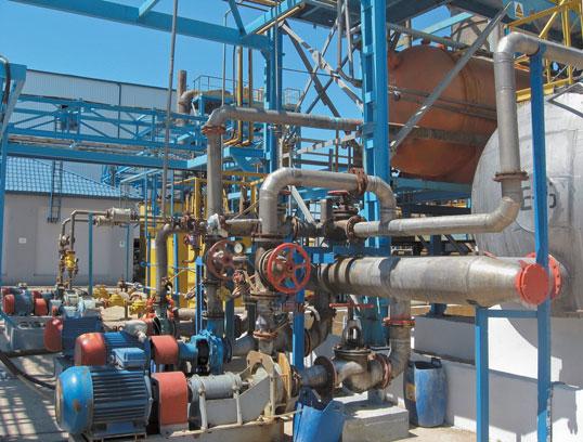
On a larger scale, consider the chemical processing plant shown in Fig. 1.1. Complex piping systems use pumps to transfer fluids from tanks and move them through various processing systems. The finished products may be stored in other tanks and then transferred to trucks or railroad cars to be delivered to customers.
Listed here are several of the major concepts you will study in this book:
■ Fluid mechanics is the study of the behavior of fluids, either at rest (fluid statics) or in motion (fluid dynamics).
■ Fluids can be either liquids or gases and they can be characterized by their physical properties such as density, specific weight, specific gravity, surface tension, and viscosity.
■ Quantitatively analyzing fluid systems requires careful use of units for all terms. Both the SI metric system of units and the U.S. gravitational system are used in this book. Careful distinction between weight and mass is also essential.
■ Fluid statics concepts that you will learn include the measurement of pressure, forces exerted on surfaces due to fluid pressure, buoyancy and stability of floating bodies.
■ Learning how to analyze the behavior of fluids as they flow through circular pipes and tubes and through conduits with other shapes is important.
■ We will consider the energy possessed by the fluid because of its velocity, elevation, and pressure.
■ Accounting for energy losses, additions, or purposeful removals that occur as the fluid flows through the
FIGURE 1.1 Industrial and commercial fluid piping systems, like this one used in a chemical processing plant, involve complex arrangements requiring careful design and analysis. (Source: Nikolay Kazachok/Fotolia)
components of a fluid flow system enables you to analyze the performance of the system.
■ A flowing fluid loses energy due to friction as it moves along a conduit and as it encounters obstructions (like in a control valve) or changes its direction (like in a pipe elbow).
■ Energy can be added to a flowing fluid by pumps that create flow and increase the fluid’s pressure.
■ Energy can be purposely removed by using it to drive a fluid motor, a turbine, or a hydraulic actuator.
■ Measurements of fluid pressure, temperature, and the fluid flow rate in a system are critical to understanding its performance.
Exploration
Now let’s consider a variety of systems that use fluids and that illustrate some of the applications of concepts learned from this book. As you read this section, consider such factors as:
■ The basic function or purpose of the system
■ The kind of fluid or fluids that are in the system
■ The kinds of containers for the fluid or the conduits through which it flows
■ If the fluid flows, what causes the flow to occur? Describe the flow path.
■ What components of the system resist the flow of the fluid?
■ What characteristics of the fluid are important to the proper performance of the system?
1. In your home, you use water for many different purposes such as drinking, cooking, bathing, cleaning, and watering lawns and plants. Water also eliminates wastes from the home through sinks, drains, and toilets. Rain water, melting snow, and water in the ground must be managed to conduct it away from the home using gutters, downspouts, ditches, and sump pumps. Consider how the water is delivered to your home. What is the ultimate source of the water—a river, a reservoir, or natural groundwater? Is the water stored in tanks at some points in the process of getting it to your home? Notice that the water system needs to be at a fairly high pressure to be effective for its uses and to flow reliably through the system. How is that pressure created? Are there pumps in the system? Describe their function and how they operate. From where does each pump draw the water? To what places is the water delivered? What quantities of fluid are needed at the delivery points? What pressures are required? How is the flow of water controlled? What materials are used for the pipes, tubes, tanks, and other containers or conduits?
As you study Chapters 6–13, you will learn how to analyze and design systems in which the water flows in a pipe or a tube. Chapter 14 discusses the cases of open-channel flow such as that in the gutters that catch the rain from the roof of your home.
2. In your car, describe the system that stores gasoline and then delivers it to the car’s engine. How is the windshield washer fluid managed? Describe the cooling system and the nature of the coolant. Describe what happens when you apply the brakes, particularly as it relates to the hydraulic fluid in the braking system. The concepts in Chapters 6–13 will help you to describe and analyze these kinds of systems.
3. Consider the performance of an automated manufacturing system that is actuated by fluid power systems such as the one shown in Fig. 1.2. Describe the fluids, pumps, tubes, valves, and other components of the system. What is the function of the system? How does the fluid accomplish that function? How is energy introduced to the system and how is it dissipated away from the system?
4. Consider the kinds of objects that must float in fluids such as boats, jet skis, rafts, barges, and buoys. Why do they float? In what position or orientation do they float? Why do they maintain their orientation? The principles of buoyancy and stability are discussed in Chapter 5.
5. What examples can you think of where fluids at rest or in motion exert forces on an object? Any vessel containing a fluid under pressure should yield examples. Consider a swimming pool, a hydraulic cylinder, a dam or a retaining wall holding a fluid, a high-pressure washer system, a fire hose, wind during a tornado or a hurricane, and water flowing through a turbine to generate power. What other examples can you think of? Chapters 4, 16, and 17 discuss these cases.
FIGURE 1.2 Typical piping system for fluid power.
6. Think of the many situations in which it is important to measure the flow rate of fluid in a system or the total quantity of fluid delivered. Consider measuring the gasoline that goes into your car so you can pay for just what you get. The water company wants to know how
much water you use in a given month. Fluids often must be metered carefully into production processes in a factory. Liquid medicines and oxygen delivered to a patient in a hospital must be measured continuously for patient safety. Chapter 15 covers flow measurement.
There are many ways in which fluids affect your life. Completion of a fluid mechanics course using this book will help you understand how those fluids can be controlled. Studying this book will help you learn how to design and analyze fluid systems to determine the kind of components that should be used and their size.
1.1 OBJECTIVES
After completing this chapter, you should be able to:
1. Differentiate between a gas and a liquid.
2. Define pressure.
3. Identify the units for the basic quantities of time, length, force, mass, and temperature in the SI metric unit system and in the U.S. Customary unit system.
4. Properly set up equations to ensure consistency of units.
5. Define the relationship between force and mass.
6. Define density, specific weight, and specific gravity and the relationships among them.
7. Define surface tension.
1.2 BASIC INTRODUCTORY CONCEPTS
■ Pressure Pressure is defined as the amount of force exerted on a unit area of a substance or on a surface. This can be stated by the equation
When a liquid is held in a container, it tends to take the shape of the container, covering the bottom and the sides. The top surface, in contact with the atmosphere above it, maintains a uniform level. As the container is tipped, the liquid tends to pour out.
When a gas is held under pressure in a closed container, it tends to expand and completely fill the container. If the container is opened, the gas tends to expand more and escape from the container.
In addition to these familiar differences between gases and liquids, another difference is important in the study of fluid mechanics. Consider what happens to a liquid or a gas as the pressure on it is increased. If air (a gas) is trapped in a cylinder with a tight-fitting, movable piston inside it, you can compress the air fairly easily by pushing on the piston. Perhaps you have used a hand-operated pump to inflate a bicycle tire, a beach ball, an air mattress, or a basketball. As you move the piston, the volume of the gas is reduced appreciably as the pressure increases. But what would happen if the cylinder contained water rather than air? You could apply a large force, which would increase the pressure in the water, but the volume of the water would change very little. This observation leads to the following general descriptions of liquids and gases that we will use in this book:
1. Gases are readily compressible.
Fluids are subjected to large variations in pressure depending on the type of system in which they are used. Milk sitting in a glass is at the same pressure as the air above it. Water in the piping system in your home has a pressure somewhat greater than atmospheric pressure so that it will flow rapidly from a faucet. Oil in a fluid power system is typically maintained at high pressure to enable it to exert large forces to actuate construction equipment or automation devices in a factory. Gases such as oxygen, nitrogen, and helium are often stored in strong cylinders or spherical tanks under high pressure to permit rather large amounts to be held in a relatively small volume. Compressed air is often used in service stations and manufacturing facilities to operate tools or to inflate tires. More discussion about pressure is given in Chapter 3.
■ Liquids and Gases Fluids can be either liquids or gases.
2. Liquids are only slightly compressible.
More discussion on compressibility is given later in this chapter. We will deal mostly with liquids in this book.
■ Weight and Mass An understanding of fluid properties requires a careful distinction between mass and weight. The following definitions apply:
Mass is the property of a body of fluid that is a measure of its inertia or resistance to a change in motion. It is also a measure of the quantity of fluid.
We use the symbol m for mass in this book.
Weight is the amount that a body of fluid weighs, that is, the force with which the fluid is attracted toward Earth by gravitation.
We use the symbol w for weight.
The relationship between weight and mass is discussed in Section 1.5 as we review the unit systems used in this book. You must be familiar with both the International System of Units, called SI, and the U.S. Customary System of units.
■ Fluid Properties The latter part of this chapter presents other fluid properties: specific weight , density , specific gravity, and surface tension. Chapter 2 presents an additional property, viscosity, which is a measure of the ease with which a fluid flows. It is also important in determining the character of the flow of fluids and the amount of energy that is lost from a fluid flowing in a system as discussed in Chapters 8–13.
1.3 THE INTERNATIONAL SYSTEM OF UNITS (SI)
In any technical work the units in which physical properties are measured must be stated. A system of units specifies the units of the basic quantities of length, time, force, and mass. The units of other terms are then derived from these.
The ultimate reference for the standard use of metric units throughout the world is the International System of Units (Système International d’Unités), abbreviated as SI. In the United States, the standard is given in the 2008 publication of the National Institute of Standards and Technology (NIST), U.S. Department of Commerce, The International System of Units (SI) (NIST Special Publication 330), edited by Barry N. Taylor and Ambler Thompson (see Reference 1). This is the standard used in this book.
The SI units for the basic quantities are
length = meter (m)
time = second (s)
mass = kilogram (kg) or N # s2/m
force = newton (N) or kg # m/s2
An equivalent unit for force is kg # m/s2, as indicated above. This is derived from the relationship between force and mass,
F = ma
where a is the acceleration expressed in units of m/s2 Therefore, the derived unit for force is
F = ma = kg # m/s2 = N
Thus, a force of 1.0 N would give a mass of 1.0 kg an acceleration of 1.0 m/s2. This means that either N or kg # m/s2 can be used as the unit for force. In fact, some calculations in this book require that you be able to use both or to convert from one to the other.
Similarly, besides using the kg as the standard unit mass, we can use the equivalent unit N # s2/m. This can be derived again from F = ma:
m = F a = N m/s2 = N # s 2 m
Therefore, either kg or N # s2/m can be used for the unit of mass.
TABLE 1.1 SI unit prefixes
Prefix SI symbol Factor
1.3.1 SI Unit Prefixes
Because the actual size of physical quantities in the study of fluid mechanics covers a wide range, prefixes are added to the basic quantities. Table 1.1 shows these prefixes. Standard usage in the SI system calls for only those prefixes varying in steps of 103 as shown. Results of calculations should normally be adjusted so that the number is between 0.1 and 10 000 times some multiple of 103.* Then the proper unit with a prefix can be specified. Note that some technical professionals and companies in Europe often use the prefix centi, as in centimeters, indicating a factor of 10−2. Some examples follow showing how quantities are given in this book.
0.004 23 m 4.23 * 10 - 3 m, or 4.23 mm (millimeters) 15 700 kg 15.7 * 103 kg, or 15.7 Mg (megagrams) 86 330 N 86.33 * 103 N, or 86.33 kN (kilonewtons)
1.4 THE U.S. CUSTOMARY SYSTEM
Sometimes called the English gravitational unit system or the pound-foot-second system, the U.S. Customary System defines the basic quantities as follows:
length = foot (ft)
time = second (s)
force = pound (lb)
mass = slug or lb s2/ft
Probably the most difficult of these units to understand is the slug because we are more familiar with measuring in
*Because commas are used as decimal markers in many countries, we will not use commas to separate groups of digits. We will separate the digits into groups of three, counting both to the left and to the right from the decimal point, and use a space to separate the groups of three digits. We will not use a space if there are only four digits to the left or right of the decimal point unless required in tabular matter.
terms of pounds, seconds, and feet. It may help to note the relationship between force and mass,
F = ma
where a is acceleration expressed in units of ft/s2. Therefore, the derived unit for mass is
m = F a = lb ft/s2 = lb s 2 ft = slug
This means that you may use either slugs or lb s2/ft for the unit of mass. In fact, some calculations in this book require that you be able to use both or to convert from one to the other.
1.5 WEIGHT AND MASS
A rigid distinction is made between weight and mass in this book. Weight is a force and mass is the quantity of a substance. We relate these two terms by applying Newton’s law of gravitation stated as force equals mass times acceleration, or
F = ma
When we speak of weight w, we imply that the acceleration is equal to g, the acceleration due to gravity. Then Newton’s law becomes
➭ Weight–Mass Relationship
w = mg (1–2)
In this book, we will use g = 9.81 m/s2 in the SI system and g = 32.2 ft/s2 in the U.S. Customary System. These are the standard values on Earth for g to three significant digits. To a greater degree of precision, we have the standard values g = 9.806 65 m/s2 and g = 32.1740 ft/s2. For highprecision work and at high elevations (such as aerospace operations) where the actual value of g is different from the standard, the local value should be used.
1.5.1 Weight and Mass in the SI Unit System
For example, consider a rock with a mass of 5.60 kg suspended by a wire. To determine what force is exerted on the wire, we use Newton’s law of gravitation (w = mg):
w = mg = mass * acceleration due to gravity
Under standard conditions, however, g = 9.81 m/s2. Then, we have
w = 5.60 kg * 9.81 m/s2 = 54.9 kg # m/s2 = 54.9 N
Thus, a 5.60 kg rock weighs 54.9 N.
We can also compute the mass of an object if we know its weight. For example, assume that we have measured the weight of a valve to be 8.25 N. What is its mass? We write
w = mg
m = w g = 8.25 N 9.81 m/s2 = 0.841 N # s 2 m = 0.841 kg
1.5.2 Weight and Mass in the U.S. Customary Unit System
For an example of the weight–mass relationship in the U.S. Customary System, assume that we have measured the weight of a container of oil to be 84.6 lb. What is its mass? We write
w = mg
1.5.3 Mass Expressed as lbm (Pounds-Mass)
In the analysis of fluid systems, some professionals use the unit lbm (pounds-mass) for the unit of mass instead of the unit of slugs. In this system, an object or a quantity of fluid having a weight of 1.0 lb has a mass of 1.0 lbm. The pound-force is then sometimes designated lbf. It must be noted that the numerical equivalence of lbf and lbm applies only when the value of g is equal to the standard value.
This system is avoided in this book because it is not a coherent system. When one tries to relate force and mass units using Newton’s law, one obtains
F = ma = lbm(ft/s2) = lbm ft/s2
This is not the same as the lbf.
To overcome this difficulty, a conversion constant, commonly called gc , is defined having both a numerical value and units. That is,
gc = 32.2 lbm lbf/(ft/s2) = 32.2 lbm ft/s2 lbf
Then, to convert from lbm to lbf, we use a modified form of Newton’s law:
F = m(a > gc)
Letting the acceleration a = g, we find
F = m(g > gc)
For example, to determine the weight of material in lbf that has a mass of 100 lbm, and assuming that the local value of g is equal to the standard value of 32.2 ft/s2, we have
w = F = m g gc = 100 lbm
32.2 ft/s2
32.2
This shows that weight in lbf is numerically equal to mass in lbm provided g = 32.2 ft/s2
If the analysis were to be done for an object or fluid on the Moon, however, where g is approximately 1/6 of that on Earth, 5.4 ft/s2, we would find w = F = m g gc = 100 lbm 5.4 ft/s2
32.2 lbm ft/s2 lbf = 16.8 lbf
This is a dramatic difference.
In summary, because of the cumbersome nature of the relationship between lbm and lbf, we avoid the use of lbm in this book. Mass will be expressed in the unit of slugs when problems are in the U.S. Customary System of units.
1.6 TEMPERATURE
Temperature is most often indicated in °C (degrees Celsius) or °F (degrees Fahrenheit). You are probably familiar with the following values at sea level on Earth:
Water freezes at 0 C and boils at 100 C.
Water freezes at 32 F and boils at 212 F.
Thus, there are 100 Celsius degrees and 180 Fahrenheit degrees between the same two physical data points, and 1.0 Celsius degree equals 1.8 Fahrenheit degrees exactly. From these observations we can define the conversion procedures between these two systems as follows:
Given the temperature TF in °F, the temperature TC in °C is
TC = (TF - 32) > 1.8
Given the temperature TC in °C, the temperature TF in °F is
TF = 1.8TC + 32
For example, given TF = 180 F, we have
TC = (TF - 32) > 1.8 = (180 - 32) > 1.8 = 82.2 C
Given TC = 33 C, we have
TF = 1.8TC + 32 = 1.8(33) + 32 = 91.4 F
In this book we will use the Celsius scale when problems are in SI units and the Fahrenheit scale when they are in U.S. Customary units.
1.6.1 Absolute Temperature
The Celsius and Fahrenheit temperature scales were defined according to arbitrary reference points, although the Celsius scale has convenient points of reference to the properties of water. The absolute temperature, on the other hand, is defined so the zero point corresponds to the condition where all molecular motion stops. This is called absolute zero.
In the SI unit system, the standard unit of temperature is the kelvin, for which the standard symbol is K and the reference (zero) point is absolute zero. Note that there is no degree symbol attached to the symbol K. The interval between points on the kelvin scale is the same as the interval used for the Celsius scale. Measurements have shown that the freezing point of water is 273.15 K above absolute zero. We can then make the conversion from the Celsius to the kelvin scale by using
TK = TC + 273.15
For example, given TC = 33 C, we have
TK = TC + 273.15 = 33 + 273.15 = 306.15 K
It has also been shown that absolute zero on the Fahrenheit scale is at - 459.67 F. In some references you will find
another absolute temperature scale called the Rankine scale, where the interval is the same as for the Fahrenheit scale. Absolute zero is 0 R and any Fahrenheit measurement can be converted to °R by using TR = TF + 459.67
Also, given the temperature in °F, we can compute the absolute temperature in K from TK = (TF + 459.67) > 1.8 = TR > 1.8
For example, given TF = 180 F, the absolute temperature in K is
The analyses required in fluid mechanics involve the algebraic manipulation of several terms. The equations are often complex, and it is extremely important that the results be dimensionally correct. That is, they must have their proper units. Indeed, answers will have the wrong numerical value if the units in the equation are not consistent. Table 1.2 summarizes standard and other common units for the quantities used in fluid mechanics.
A simple straightforward procedure called unit cancellation will ensure proper units in any kind of calculation, not only in fluid mechanics, but also in virtually all your technical work. The six steps of the procedure are listed below.
Unit-Cancellation Procedure
1. Solve the equation algebraically for the desired term.
2. Decide on the proper units for the result.
3. Substitute known values, including units.
4. Cancel units that appear in both the numerator and the denominator of any term.
5. Use conversion factors to eliminate unwanted units and obtain the proper units as decided in Step 2.
6. Perform the calculation.
This procedure, properly executed, will work for any equation. It is really very simple, but some practice may be required to use it. We are going to borrow some material from elementary physics, with which you should be familiar, to illustrate the method. However, the best way to learn how to do something is to do it. The following example problems are presented in a form called programmed instruction. You will be guided through the problems in a step-by-step fashion with your participation required at each step.
To proceed with the program you should cover all material under the heading Programmed Example Problem, using an opaque sheet of paper or a card. You should have a blank piece of paper handy on which to perform the requested operations. Then successively uncover one panel at a time down to the heavy line that runs across the page. The first panel presents a problem and asks you to perform
TABLE 1.2 Units for common quantities used in fluid mechanics in SI units and U.S. Customary units
flow rate (W) w/time
Mass flow rate (M) M/time
Specific weight (g) w/V N/m3 or kg/m2·s2 lb/ft3
Density (r) M/V kg/m3 or N·s2/m4 slugs/ft3
some operation or to answer a question. After doing what is asked, uncover the next panel, which will contain information that you can use to check your result. Then continue with the next panel, and so on through the program.
Remember, the purpose of this is to help you learn how to get correct answers using the unit-cancellation method. You may want to refer to the table of conversion factors in Appendix K.
PROGRAMMED EXAMPLE PROBLEM
Example Problem 1.1
Imagine you are traveling in a car at a constant speed of 80 kilometers per hour (km/h). How many seconds (s) would it take to travel 1.5 km?
For the solution, use the equation
s = vt
where s is the distance traveled, y is the speed, and t is the time. Using the unit-cancellation procedure outlined above, what is the first thing to do?
The first step is to solve for the desired term. Because you were asked to find time, you should have written
t = s v
Now perform Step 2 of the procedure described above.
Step 2 is to decide on the proper units for the result, in this case time. From the problem statement the proper unit is seconds. If no specification had been given for units, you could choose any acceptable time unit such as hours.