The Advantages of MATLAB for Technical Programming
MATLAB has many advantages compared to conventional computer languages for technical problem solving. Among them are:
1. Ease of use.
MATLAB is an interpreted language, like many versions of Basic. Like Basic, it is very easy to use. The program can be used as a scratch pad to evaluate expressions typed at the command line, or it can be used to execute large prewritten programs. Programs may be easily written and modi ed with the built-in integrated development environment, and debugged with the MATLAB debugger. Because the language is so easy to use, it is ideal for educational use, and for the rapid prototyping of new programs.
Many program development tools are provided to make the program easy to use. They include an integrated editor/debugger, online documentation and manuals, a workspace browser, and extensive demos.
2. Platform independence.
MATLAB is supported on many different computer systems, and this provides a large measure of platform independence. At the time of this writing, the language is supported on Windows 7/8/10, Linux, and Mac OS X 10.10 and 10.11. Programs written on any platform will run on all of the other platforms, and data les written on any platform may be read transparently on any other platform. As a result, programs written in MATLAB can migrate to new platforms when the needs of the user change.
3. Prede ned functions.
MATLAB comes complete with an extensive library of prede ned functions that provide tested and prepackaged solutions to many basic technical tasks. For example, suppose that you are writing a program that must calculate the statistics associated with an input data set. In most languages, you would need to write your own subroutines or functions to implement calculations such as the arithmetic mean, standard deviation, median, etc. These and hundreds of other functions are built right into the MATLAB language, making your job much easier.
In addition to the large library of functions built into the basic MATLAB language, there are many special-purpose toolboxes available to help solve complex problems in speci c areas. For example, a user can buy standard toolboxes to solve problems in Signal Processing, Control Systems, Communications, Image Processing, and Neural Networks, among many others.
4. Device-independent plotting.
Unlike other computer languages, MATLAB has many integral plotting and imaging commands. The plots and images can be displayed on any graphical output device supported by the computer on which MATLAB is running. This capability makes MATLAB an outstanding tool for visualizing technical data.
5. Graphical user interface.
MATLAB includes tools that allow a programmer to interactively construct a graphical user interface (GUI) for his or her program. With this capability, the programmer can design sophisticated data analysis programs that can be operated by relatively inexperienced users.
Pedagogical Features
This book is speci cally designed to be used in a rst-year “Introduction to Programming/Problem Solving” course. It should be possible to cover this material comfortably in a 9-week, 3-hour-per-week course. If there is insuf cient time to cover all of the material in a particular engineering program, Chapters 8 and 9 may be deleted, and the remaining material will still teach the fundamentals of programming and using MATLAB to solve problems. This feature should appeal to harassed engineering educators trying to cram ever more material into a nite curriculum.
The book includes several features designed to aid student comprehension. A total of 14 quizzes appear scattered throughout the chapters, with answers to all questions included in Appendix C. These quizzes can serve as a useful self-test of comprehension. In addition, there are approximately 150 end-ofchapter exercises. Answers to all exercises are included in the Instructor’s Manual. Good programming practices are highlighted in all chapters with special Good Programming Practice boxes, and common errors are highlighted in Programming Pitfalls boxes. End-of-chapter materials include Summaries of Good Programming Practice and Summaries of MATLAB Commands and Functions.
Instructor Resources
A detailed Instructor’s Solutions Manual containing solutions to all end-ofchapter exercises is available via the secure, password-protected Instructor Resource Center at https://sso.cengage.com. The Instructor Resource Center also contains helpful Lecture Note PowerPoint slides, the MATLAB source code for all examples in the book, and the source code for all of the solutions in the Instructor’s Solutions Manual.
A Final Note to the User
No matter how hard I try to proofread a document like this book, it is inevitable that some typographical errors will slip through and appear in print. If you should spot any such errors, please drop me a note via the publisher at globalengineering@cengage.com, and I will do my best to get them eliminated from subsequent printings and editions. Thank you very much for your help in this matter.
I will maintain a complete list of errata and corrections at the Instructor Resource Center mentioned above. Please check that site for any updates and/ or corrections.
Acknowledgments
I would like to thank these reviewers who offered their helpful suggestion for this edition:
David Eromom
Arlene Guest
Georgia Southern University
Naval Postgraduate School
Mary M. Ho e Idaho State University
Mark Hutchenreuther California Polytechnic State University
Mani Mini Iowa State University
In addition I would like to acknowledge and thank my Global Engineering team at Cengage Learning for their dedication to this edition: Timothy Anderson, Product Director; Mona Zeftel, Senior Content Developer; D. Jean Buttrom, Content Project Manager; Kristin Stine, Marketing Manager; Elizabeth Murphy and Brittany Burden, Learning Solutions Specialists; Ashley Kaupert, Associate Media Content Developer; Teresa Versaggi and Alexander Sham, Product Assistants; and Rose Kernan of RPK Editorial Services, Inc. They have skillfully guided every aspect of this text’s development and production to successful completion.
In addition, I would like to thank my wife Rosa for her help and encouragement over the more than 40 years we have spent together.
Stephen J. Chapman
Melbourne, Australia November 8, 2015
MindTap Online Course
Essentials of MATLAB Programming is also available through MindTap, Cengage Learning’s digital course platform. The carefully-crafted pedagogy and exercises in this trusted textbook are made even more effective by an interactive, customizable eBook, automatically graded assessments, and a full suite of study tools.
As an instructor using MindTap, you have at your ngertips the full text and a unique set of tools, all in an interface designed to save you time. MindTap makes it easy for instructors to build and customize their course, so you can focus on the most relevant material while also lowering costs for your students. Stay connected and informed through realtime student tracking that provides the opportunity to adjust your course as needed based on analytics of interactivity and performance. End-of-chapter assessments test students’ knowledge of programming concepts in each chapter. Tutorial videos help students master MATLAB functionality, programming, and concepts.
How does MindTap bene t instructors?
■ You can build and personalize your course by integrating your own content into the MindTap Reader (like lecture notes or problem sets to download) or pull from sources such as RSS feeds, YouTube videos, websites, and more. Control what content students see with a built-in learning path that can be customized to your syllabus.
■ MindTap saves you time by providing you and your students with automatically graded assignments and quizzes. These problems include immediate, speci c feedback, so students know exactly where they need more practice.
■ The Message Center helps you to quickly and easily contact students directly from MindTap. Messages are communicated directly to each student via the communication medium (email, social media, or even text message) designated by the student.
■ StudyHub is a valuable studying tool that allows you to deliver important information and empowers your students to personalize their experience. Instructors can choose to annotate the text with notes and highlights, share content from the MindTap Reader, and create ashcards to help their students focus and succeed.
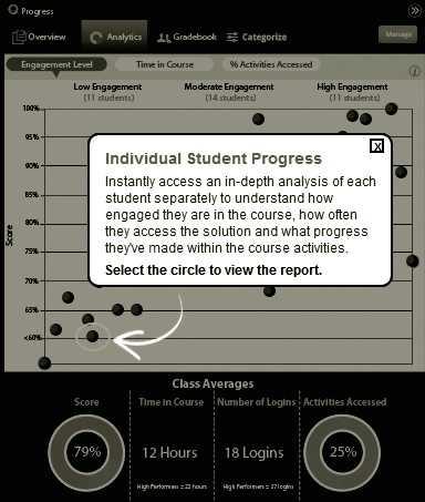
■ The Progress App lets you know exactly how your students are doing (and where they might be struggling) with live analytics. You can see overall class engagement and drill down into individual student performance, enabling you to adjust your course to maximize student success.
How does MindTap bene t your students?
■ The MindTap Reader adds the abilities to have the content read aloud, to print from the reader, and to take notes and highlights while also capturing them within the linked StudyHub App.
■ The MindTap Mobile App keeps students connected with alerts and noti cations while also providing them with on-the-go study tools like Flashcards and quizzing, helping them manage their time ef ciently.
■ Flashcards are pre-populated to provide a jump start on studying, and students and instructors can also create customized cards as they move through the course.
■ The Progress App allows students to monitor their individual grades, as well as their level compared to the class average. This not only helps them stay on track in the course but also motivates them to do more, and ultimately to do better.
■ The unique StudyHub is a powerful single-destination studying tool that empowers students to personalize their experience. They can quickly and easily access all notes and highlights marked in the MindTap Reader, locate bookmarked pages, review notes and Flashcards shared by their instructor, and create custom study guides.
For more information about MindTap for Engineering, or to schedule a demonstration, please call (800) 354-9706 or email higheredcs@cengage.com. For those instructors outside the United States, please visit http://www.cengage.com/contact/ to locate your regional of ce.
Contents
Chapter 1 Introduction to MATLAB 1
1.1 The Advantages of MATLAB 2
1.2 Disadvantages of MATLAB 3
1.3 The MATLAB Environment 4
1.3.1 The MATLAB Desktop 4
1.3.2 The Command Window 6
1.3.3 The Toolstrip 7
1.3.4 The Command History Window 8
1.3.5 The Document Window 8
1.3.6 Figure Windows 11
1.3.7 Docking and Undocking Windows 12
1.3.8 The MATLAB Workspace 12
1.3.9 The Workspace Browser 14
1.3.10 The Current Folder Browser 15
1.3.11 Getting Help 16
1.3.12 A Few Important Commands 18
1.3.13 The MATLAB Search Path 19
1.4 Using MATLAB as a Calculator 21
1.5 Summary 23
1.5.1 MATLAB Summary 23
1.6 Exercises 24
Chapter 2 MATLAB Basics 27
2.1 Variables and Arrays 27
2.2 Creating and Initializing Variables in MATLAB 31
2.2.1 Initializing Variables in Assignment Statements 31
2.2.2 Initializing with Shortcut Expressions 34
2.2.3 Initializing with Built-in Functions 35
2.2.4 Initializing Variables with Keyboard Input 36
2.3 Multidimensional Arrays 38
2.3.1 Storing Multidimensional Arrays in Memory 39
2.3.2 Accessing Multidimensional Arrays with One Dimension 40
2.4 Subarrays 40
2.4.1 The end Function 41
2.4.2 Using Subarrays on the Left-Hand Side of an Assignment Statement 41
2.4.3 Assigning a Scalar to a Subarray 43
2.5 Special Values 43
2.6 Displaying Output Data 46
2.6.1 Changing the Default Format 46
2.6.2 The disp Function 48
2.6.3 Formatted Output with the fprintf Function 48
2.7 Data Files 49
2.8 Scalar and Array Operations 52
2.8.1 Scalar Operations 52
2.8.2 Array and Matrix Operations 53
2.9 Hierarchy of Operations 56
2.10 Built-in MATLAB Functions 59
2.10.1 Optional Results 60
2.10.2 Using MATLAB Functions with Array Inputs 60
2.10.3 Common MATLAB Functions 60
2.11 Introduction to Plotting 62
2.11.1 Using Simple xy Plots 62
2.11.2 Printing a Plot 63
2.11.3 Exporting a Plot as a Graphical Image 64
2.11.4 Multiple Plots 66
2.11.5 Line Color, Line Style, Marker Style, and Legends 67
2.11.6 Logarithmic Scales 70
2.12 Examples 71
2.13 Debugging MATLAB Programs 78 2.14 Summary 80
2.14.1 Summary of Good Programming Practice 81
2.14.2 MATLAB Summary 82
2.15 Exercises 85
Chapter 3 Two-Dimensional Plots 93
3.1 Additional Plotting Features for Two-Dimensional Plots 93
3.1.1 Logarithmic Scales 93
3.1.2 Controlling x- and y-axis Plotting Limits 97
3.1.3 Plotting Multiple Plots on the Same Axes 100
3.1.4 Creating Multiple Figures 101
3.1.5 Subplots 101
3.1.6 Controlling the Spacing between Points on a Plot 104
3.1.7 Enhanced Control of Plotted Lines 107
3.1.8 Enhanced Control of Text Strings 108
3.2 Polar Plots 111
3.3 Annotating and Saving Plots 113
3.4 Additional Types of Two-Dimensional Plots 116
3.5 Using the plot Function with Two-Dimensional Arrays 121
3.6 Summary 123
3.6.1 Summary of Good Programming Practice 124
3.6.2 MATLAB Summary 124
3.7 Exercises 125
Chapter 4 Branching Statements and Program Design 129
4.1 Introduction to Top-Down Design Techniques 129
4.2 Use of Pseudocode 133
4.3 The Logical Data Type 134
4.3.1 Relational and Logic Operators 134
4.3.2 Relational Operators 135
4.3.3 A Caution about the == and ~= Operators 136
4.3.4 Logic Operators 137
4.3.5 Logical Functions 142
4.4 Branches 144
4.4.1 The if Construct 144
4.4.2 Examples Using if Constructs 146
4.4.3 Notes Concerning the Use of if Constructs 152
4.4.4 The switch Construct 155
4.4.5 The try/catch Construct 156
4.5 More on Debugging MATLAB Programs 164
4.6 Summary 171
4.6.1 Summary of Good Programming Practice 171
4.6.2 MATLAB Summary 172
4.7 Exercises 172
Chapter 5 Loops and Vectorization 179
5.1 The while Loop 179
5.2 The for Loop 185
5.2.1 Details of Operation 192
5.2.2 Vectorization: A Faster Alternative to Loops 194
5.2.3 The MATLAB Just-In-Time (JIT) Compiler 195
5.2.4 The break and continue Statements 198
5.2.5 Nesting Loops 200
5.3 Logical Arrays and Vectorization 201
5.3.1 Creating the Equivalent of if/else Constructs with Logical Arrays 202
5.4 The MATLAB Pro ler 204
5.5 Additional Examples 207
5.6 The textread Function 222
5.7 Summary 223
5.7.1 Summary of Good Programming Practice 224
5.7.2 MATLAB Summary 224
5.8 Exercises 225
Chapter 6 Basic User - De ned Functions 235
6.1 Introduction to MATLAB Functions 236
6.2 Variable Passing in MATLAB: T he Pass-by-Value Scheme 242
6.3 Optional Arguments 253
6.4 Sharing Data Using Global Memory 258
6.5 Preserving Data between Calls to a Function 265
6.7 Built-in MATLAB Functions: Random Number Functions 272
6.8 Summary 272
6.8.1 Summary of Good Programming Practice 273
6.8.2 MATLAB Summary 273
6.9 Exercises 274
Chapter 7 Advanced Features of User-De ned Functions 283
7.1 Function Functions 283
7.2 Local Functions, Private Functions, and Nested Functions 288
7.2.1 Local Functions 288
7.2.2 Private Functions 289
7.2.3 Nested Functions 290
7.2.4 Order of Function Evaluation 292
7.3 Function Handles 293
7.3.1 Creating and Using Function Handles 293
7.3.2 The Signi cance of Function Handles 296
7.3.3 Function Handles and Nested Functions 297
7.3.4 An Example Application: Solving Ordinary Differential Equations 299
7.4 Anonymous Functions 305
7.5 Recursive Functions 306
7.6 Plotting Functions 307
7.7 Histograms 310
7.8 Summary 316
7.8.1 Summary of Good Programming Practice 316
7.8.2 MATLAB Summary 317
7.9 Exercises 317
Chapter 8 Additional Data Types and Plot Types 325
8.1 Complex Data 325
8.1.1 Complex Variables 327
8.1.2 Using Complex Numbers with Relational Operators 328
8.1.3 Complex Functions 329
8.1.4 Plotting Complex Data 334
8.2 Strings and String Functions 338
8.2.1 String Conversion Functions 338
8.2.2 Creating Two-Dimensional Character Arrays 339
8.2.3 Concatenating Strings 340
8.2.4 Comparing Strings 340
8.2.5 Searching/Replacing Characters within a String 344
8.2.6 Uppercase and Lowercase Conversion 345
8.2.7 Trimming Whitespace from Strings 345
8.2.8 Numeric-to-String Conversions 346
8.2.9 String-to-Numeric Conversions 348
8.2.10 Summary 349
8.3 Multidimensional Arrays 355
8.4 Three-Dimensional Plots 357
8.4.1 Three-Dimensional Line Plots 357
8.4.2 Three-Dimensional Surface, Mesh, and Contour Plots 358
8.4.3 Creating Three-Dimensional Objects Using Surface and Mesh Plots 365
8.5 Summary 368
8.5.1 Summary of Good Programming Practice 368
8.5.2 MATLAB Summary 369
8.6 Exercises 371
Chapter 9 Cell Arrays, Structures, and Handle Graphics 377
9.1 Cell Arrays 377
9.1.1 Creating Cell Arrays 379
9.1.2 Using Braces {} as Cell Constructors 380
9.1.3 Viewing the Contents of Cell Arrays 381
9.1.4 Extending Cell Arrays 381
9.1.5 Deleting Cells in Arrays 384
9.1.6 Using Data in Cell Arrays 385
9.1.7 Cell Arrays of Strings 385
9.1.8 The Signi cance of Cell Arrays 386
9.1.9 Summary of cell Functions 390
9.2 Structure Arrays 391
9.2.1 Creating Structure Arrays 391
9.2.2 Adding Fields to Structures 394
9.2.3 Removing Fields from Structures 395
9.2.4 Using Data in Structure Arrays 395
9.2.5 The getfield and setfield Functions 397
9.2.6 Dynamic Field Names 397
9.2.7 Using the size Function with Structure Arrays 399
9.2.8 Nesting Structure Arrays 399
9.2.9 Summary of structure Functions 400
9.3 Handle Graphics 401
9.3.1 The MATLAB Graphics System 402
9.3.2 Object Handles 403
9.3.3 Examining and Changing Object Properties 404
9.3.4 Changing Object Properties at Creation Time 404
9.3.5 Changing Object Properties after Creation Time 405
9.3.6 Examining and Changing Properties Using Object Notation 405
9.3.7 Examining and Changing Properties Using get/set Functions 407
9.3.8 Examining and Changing Properties Using the Property Editor 409
9.3.9 Using set to List Possible Property Values 414
9.3.10 Finding Objects 415
9.3.11 Selecting Objects with the Mouse 417
9.4 Position and Units 420
9.4.1 Positions of figure Objects 420
9.4.2 Positions of axes and uicontrol Objects 421
9.4.3 Positions of text Objects 422
9.5 Printer Positions 425
9.6 Default and Factory Properties 425
9.7 Graphics Object Properties 427
9.8 Summary 428
9.8.1 Summary of Good Programming Practice 428
9.8.2 MATLAB Summary 429
9.9 Exercises 429
Appendix A UTF-8 Character Set 433
Appendix B MATLAB Input/Output Functions 435
Appendix C Answers to Quizzes 457
Appendix D MATLAB Functions and Commands 471
Index 479
Chapter 1 Introduction to MATLAB
MATLAB (short for MATrix LABoratory) is a special-purpose computer program optimized to perform engineering and scienti c calculations. It started life as a program designed to perform matrix mathematics, but over the years it has grown into a exible computing system capable of solving essentially any technical problem.
The MATLAB program implements the MATLAB programming language and provides a very extensive library of prede ned functions to make technical programming tasks easier and more ef cient. This book introduces the MATLAB language as it is implemented in MATLAB Version 2014B and shows how to use it to solve typical technical problems.
MATLAB is a huge program, with an incredibly rich variety of functions. Even the basic version of MATLAB without any toolkits is much richer than other technical programming languages. There are more than 1000 functions in the basic MATLAB product alone, and the toolkits extend this capability with many more functions in various specialties. Furthermore, these functions often solve very complex problems (solving differential equations, inverting matrices, and so forth) in a single step, saving large amounts of time. Doing the same thing in another computer language usually involves writing complex programs yourself or buying a third-party software package (such as IMSL or the NAG software libraries) that contains the functions.
The built-in MATLAB functions are almost always better than anything that an individual engineer could write on his or her own because many people have worked on them, and they have been tested against many different data sets. These functions are also robust, producing sensible results for wide ranges of input data and gracefully handling error conditions.
This book makes no attempt to introduce the user to all of MATLAB’s functions. Instead, it teaches a user the basics of how to write, debug, and optimize good MATLAB programs, plus a subset of the most important functions used to solve common scienti c and engineering problems. Just as importantly, it teaches
the scientist or engineer how to use MATLAB’s own tools to locate the right function for a speci c purpose from the enormous list of choices available. In addition, it teaches how to use MATLAB to solve many practical engineering problems, such as vector and matrix algebra, curve tting, differential equations, and data plotting.
The MATLAB program is a combination of a procedural programming language, an integrated development environment (IDE) including an editor and debugger, and an extremely rich set of functions to perform many types of technical calculations.
The MATLAB language is a procedural programming language, meaning that the engineer writes procedures, which are effectively mathematical recipes for solving a problem. This makes MATLAB very similar to other procedural languages such as C, Basic, Fortran, and Pascal. However, the extremely rich list of prede ned functions and plotting tools makes it superior to these other languages for many engineering analysis applications.
1.1 The Advantages of MATLAB
MATLAB has many advantages compared to conventional computer languages for technical problem solving. Among them are:
1. Ease of use.
MATLAB is an interpreted language, like many versions of Basic. Like Basic, it is very easy to use. The program can be used as a scratch pad to evaluate expressions typed at the command line, or it can be used to execute large prewritten programs. Programs may be easily written and modi ed with the built-in integrated development environment and debugged with the MATLAB debugger. Because the language is so easy to use, it is ideal for the rapid prototyping of new programs.
Many program development tools are provided to make the program easy to use. They include an integrated editor/debugger, online documentation and manuals, a workspace browser, and extensive demos.
2. Platform independence.
MATLAB is supported on many different computer systems, providing a large measure of platform independence. At the time of this writing, the language is supported on Windows Vista/7/8/10, Linux, Unix and the Macintosh. Programs written on any platform will run on all of the other platforms, and data les written on any platform may be read transparently on any other platform. As a result, programs written in MATLAB can migrate to new platforms when the needs of the user change.
3. Prede ned functions.
MATLAB comes complete with an extensive library of prede ned functions that provide tested and prepackaged solutions to many basic technical tasks. For example, suppose that you are writing a program that must calculate the statistics associated with an input data set. In most languages, you would need to write your own subroutines or functions to
implement calculations such as the arithmetic mean, standard deviation, median, and so forth. These and hundreds of other functions are built right into the MATLAB language, making your job much easier.
In addition to the large library of functions built into the basic MATLAB language, there are many special-purpose toolboxes available to help solve complex problems in speci c areas. For example, a user can buy standard toolboxes to solve problems in signal processing, control systems, communications, image processing, and neural networks, among many others. There is also an extensive collection of free user-contributed MATLAB programs that are shared through the MATLAB website.
4. Device-independent plotting.
Unlike most other computer languages, MATLAB has many integral plotting and imaging commands. The plots and images can be displayed on any graphical output device supported by the computer on which MATLAB is running. This capability makes MATLAB an outstanding tool for visualizing technical data.
5. Graphical user interface.
MATLAB includes tools that allow an engineer to interactively construct a Graphical User Interface (GUI) for his or her program. With this capability, the engineer can design sophisticated data analysis programs that can be operated by relatively inexperienced users.
6. MATLAB compiler.
MATLAB’s exibility and platform independence is achieved by compiling MATLAB programs into a device-independent p-code, and then interpreting the p-code instructions at run-time. This approach is similar to that used by Microsoft’s Visual Basic or by Java. Unfortunately, the resulting programs can sometimes execute slowly because the MATLAB code is interpreted rather than compiled. Recent versions of MATLAB have partially overcome this problem by introducing just-in-time (JIT) compiler technology. The JIT compiler compiles portions of the MATLAB code as it is executed to increase overall speed.
A separate MATLAB compiler is also available. This compiler can compile a MATLAB program into a standalone executable that can run on a computer without a MATLAB license. It is a great way to convert a prototype MATLAB program into an executable suitable for sale and distribution to users.
1.2 Disadvantages of MATLAB
MATLAB has two principal disadvantages. The rst is that it is an interpreted language and therefore can execute more slowly than compiled languages. This problem can be mitigated by properly structuring the MATLAB program to maximize the performance of vectorized code and by the use of the JIT compiler.
The second disadvantage is cost: a full copy of MATLAB is ve to ten times more expensive than a conventional C or Fortran compiler. This relatively high cost is more than offset by the reduced time required for an engineer or scientist to create a working program, so MATLAB is cost-effective for businesses. However, it is too expensive for most individuals to consider purchasing. Fortunately, there is also an inexpensive student edition of MATLAB, which is a great tool for students wishing to learn the language. The student edition of MATLAB is essentially identical to the full edition.1
1.3 The MATLAB Environment
The fundamental unit of data in any MATLAB program is the array. An array is a collection of data values organized into rows and columns and known by a single name. Individual data values within an array can be accessed by including the name of the array followed by subscripts in parentheses, which identify the row and column of the particular value. Even scalars are treated as arrays by MATLAB—they are simply arrays with only one row and one column. We will learn how to create and manipulate MATLAB arrays in Section 1.4.
When MATLAB executes, it can display several types of windows that accept commands or display information. The three most important types of windows are the Command Window, where commands may be entered; gure windows, which display plots and graphs; and edit windows, which permit a user to create and modify MATLAB programs. We will see examples of all three types of windows in this section.
In addition, MATLAB can display other windows that provide help and that allow the user to examine the values of variables de ned in memory. We will examine some of these additional windows here and examine the others when we discuss how to debug MATLAB programs.
1.3.1 The MATLAB Desktop
When you start MATLAB Version 2014B, a special window called the MATLAB desktop appears. The desktop is a window that contains other windows showing MATLAB data, plus toolbars and a “Toolstrip” or “Ribbon Bar” similar to that used by Microsoft Of ce. By default, most MATLAB tools are docked to the desktop, so that they appear inside the desktop window. However, the user can choose to undock any or all tools, making them appear in windows separate from the desktop.
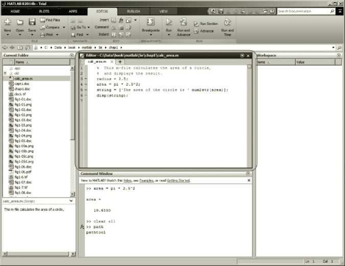
The default con guration of the MATLAB desktop is shown in Figure 1.1. It integrates many tools for managing les, variables, and applications within the MATLAB environment.
1There are also some free software programs that are largely compatible with MATLAB, such as GNU Octave and FreeMat.
Current Folder Browser shows a list of the files in the current directory
This control allow a user to view or change the current directory
Launch the Help Browser
MATLAB Editor
Details Window displays the properties of a file selected in the Current Folder Browser
MATLAB Command Window
Workspace Browser shows variables defined in workspace
Figure 1.1 The default MATLAB desktop. The exact appearance of the desktop may differ slightly on different types of computers.
The major tools within or accessible from the MATLAB desktop are:
■ Command Window
■ Toolstrip
■ Documents Window, including the Editor/Debugger and Array Editor
■ Figure Windows
■ Workspace Browser
■ Current Folder Browser, with the Details Window
■ Help Browser
■ Path Browser
■ Popup Command History Window
Table 1.1: Tools and Windows Included in the MATLAB Desktop
Tool
Command Window
Toolstrip
Command History Window
Document Window
Figure Window
Workspace Browser
Current Folder Browser
Help Browser
Path Browser
Description
A window where the user can type commands and see immediate results
A strip across the top of the desktop containing icons to select functions and tools, arranged in tabs and sections of related functions
A window that displays recently used commands, accessed by clicking the up arrow when typing in the Command Window
A window that displays MATLAB les and allows the user to edit or debug them
A window that displays a MATLAB plot
A window that displays the names and values of variables stored in the MATLAB Workspace
A window that displays the names of les in the current directory. If a le is selected in the Current Folder Browser, details about the le will appear in the Details Window
A tool to get help for MATLAB functions, accessed by clicking the Help button
A tool to display the MATLAB search path, accessed by clicking the Set Path button
The functions of these tools are summarized in Table 1.1. We will discuss them in later sections of this chapter.
1.3.2 The Command Window
The bottom center of the default MATLAB desktop contains the Command Window. A user can enter interactive commands at the command prompt (») in the Command Window, and they will be executed on the spot.
As an example of a simple interactive calculation, suppose that you want to calculate the area of a circle with a radius of 2.5 m. This can be done in the MATLAB Command Window by typing:
» area = pi * 2.5^2
area = 19.6350
MATLAB calculates the answer as soon as the Enter key is pressed, and stores the answer in a variable (really a 1 3 1 array) called area. The contents of the variable are displayed in the Command Window as shown in Figure 1.2, and
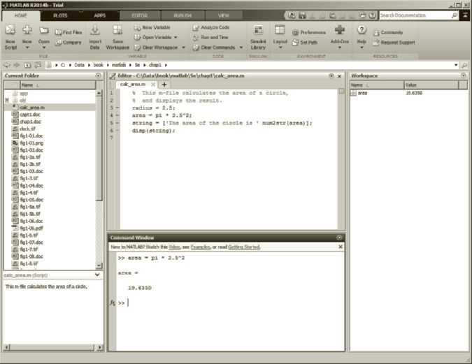
Figure 1.2 The Command Window appears in the center of the desktop. Users enter commands and see responses here.
the variable can be used in further calculations. (Note that is prede ned in MATLAB, so we can just use pi without rst declaring it to be 3.141592. . . .)
If a statement is too long to type on a single line, it may be continued on successive lines by typing an ellipsis ( ) at the end of the rst line, and then continuing on the next line. For example, the following two statements are identical.
x1 = 1 + 1/2 + 1/3 + 1/4 + 1/5 + 1/6 and
x1 = 1 + 1/2 + 1/3 + 1/4 ... + 1/5 + 1/6
Instead of typing commands directly in the Command Window, a series of commands can be placed into a le, and the entire le can be executed by typing its name in the Command Window. Such les are called script les. Script les (and functions, which we will see later) are also known as M- les, because they have a le extension of “.m”.
1.3.3
The Toolstrip
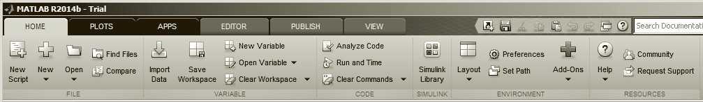
The Toolstrip (see Figure 1.3) is a bar of tools that appears across the top of the desktop. The controls on the Toolstrip are organized into related categories of functions, rst by tabs and then by groups. For example, the tabs visible in
User input
Result of calculation
Result is added to the workspace
Figure 1.3 The Toolstrip, which allows a user to select from a wide variety of MATLAB tools and commands.
Figure 1.3 are Home, Plots, Apps, Editor, and so forth. When one of the tabs is selected, a series of controls grouped into sections is displayed. In the Home tab, the sections are File, Variable, Code, and so forth. With practice, the logical grouping of commands helps the user to quickly locate any desired function. In addition, the upper right-hand corner of the Toolstrip contains the Quick Access Toolbar, which is a place where the user can customize the interface and display the most commonly used commands and functions at all times. To customize the functions displayed there, right-click on the toolbar and select the Customize option from the popup menu.
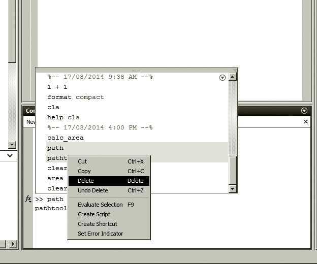
1.3.4 The Command History Window
The Command History window displays a list of the commands that a user has previously entered in the Command Window. The list of commands can extend back to previous executions of the program. Commands remain in the list until they are deleted. To display the Command History window, press the up arrow key while typing in the Command Window. To re-execute any command, simply double-click it with the left mouse button. To delete one or more commands from the Command History window, select the commands and rightclick them with the mouse. A popup menu will be displayed that allows the user to delete the items (see Figure 1.4).
1.3.5
The Document Window
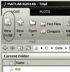
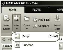
A Document Window (also called an Edit/Debug Window) is used to create new M- les or modify existing ones. An Edit Window is created automatically when you create a new M- le or open an existing one. You can create a new M- le with the New Script command from the File group on the Toolstrip (Figure 1.5a), or by clicking the New icon and selecting Script from the popup
Figure 1.4 The Command History Window, showing two commands being deleted.
menu (Figure 1.5b). You can open an existing M- le le with the Open command from the File section on the Toolstrip.
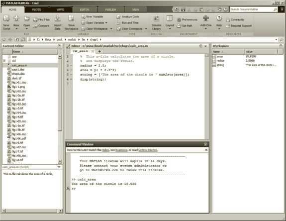
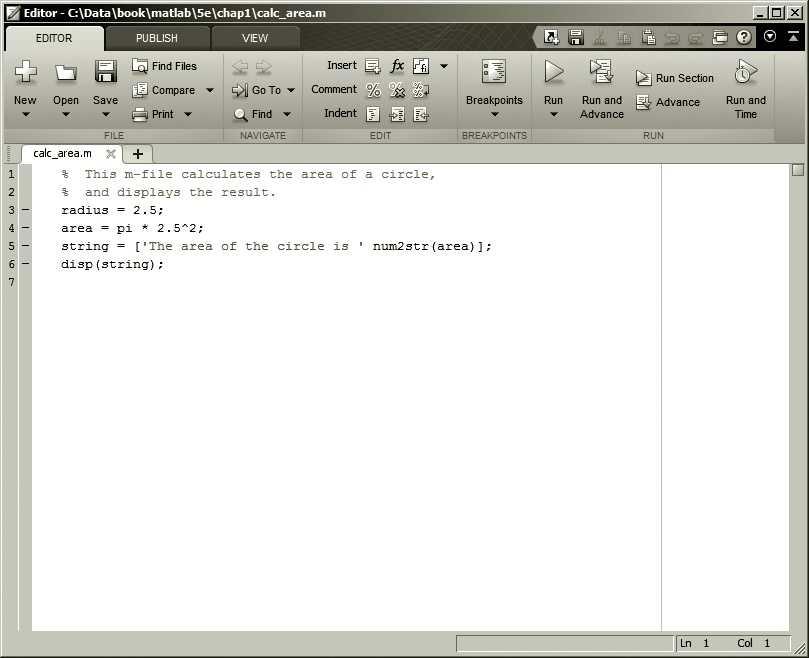
An Edit Window displaying a simple M- le called calc_area.m is shown in Figure 1.5. This le calculates the area of a circle given its radius and displays the result. By default, the Edit Window is docked to the desktop, as shown in Figure 1.5 c . The Edit Window can also be undocked from the MATLAB desktop. In that case, it appears within a container called the Documents Window, as shown in Figure 1.5 d . We will learn how to dock and undock a window later in this chapter.
The Edit Window is essentially a programming text editor, with the MATLAB language’s features highlighted in different colors. On screen, comments in an M- le le appear in green, variables and numbers appear in black, complete character strings appear in magenta, incomplete character strings appear in red, and language keywords appear in blue. [See color insert.]
After an M- le is saved, it may be executed by typing its name in the Command Window. For the M- le in Figure 1.5, the results are:
» calc_area
The area of the circle is 19.635
The Edit Window also doubles as a debugger, as we shall see in Chapter 2.
(a)
(b)
(c)
1.3.6
Figure 1.5 (a) Creating a new M- le with the New Script command. (b) Creating a new M- le with the New >> Script popup menu. (c) The MATLAB Editor, docked to the MATLAB desktop. (d) The MATLAB Editor, displayed as an independent window. [See color insert.] (d)
Figure Windows
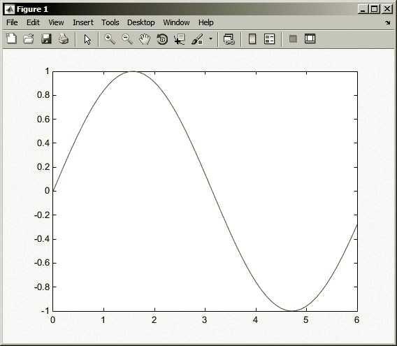
A gure window is used to display MATLAB graphics. A gure can be a two- or three-dimensional plot of data, an image, or a graphical user interface (GUI). A simple script le that calculates and plots the function sin x is shown below:
% sin_x.m: This M-file calculates and plots the % function sin(x) for 0 <= x <= 6.
x = 0:0.1:6
y = sin(x) plot(x,y)
If this le is saved under the name sin_x.m, then a user can execute the le by typing “sin_x” in the Command Window. When this script le is executed, MATLAB opens a gure window and plots the function sin x in it. The resulting plot is shown in Figure 1.6.
Figure 1.6 MATLAB plot of sin x versus x.
1.3.7 Docking and Undocking Windows
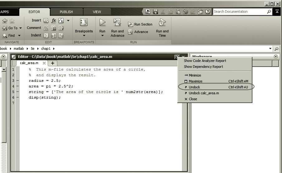
MATLAB windows such as the Command Window, the Edit Window, and Figure Windows can either be docked to the desktop, or they can be undocked. When a window is docked, it appears as a pane within the MATLAB desktop. When it is undocked, it appears as an independent window on the computer screen separate from the desktop. When a window is docked to the desktop, it can be undocked by selecting the small down arrow in the upper right-hand corner and selecting the Undock option from the popup menu (see Figure 1.7). When the window is an independent window, the upper right-hand corner contains a small button with an arrow pointing down and to the right ( ). If this button is clicked, then the window will be re-docked with the desktop. The Dock button is visible in the upper-right corner of Figure 1.6.
1.3.8 The MATLAB Workspace
A statement like z = 10
creates a variable named z, stores the value 10 in it, and saves it in a part of computer memory known as the workspace. A workspace is the collection of all the variables and arrays that can be used by MATLAB when a particular command, M- le, or function is executing. All commands executed in the Command
Figure 1.7 Select the Undock option from the menu displayed after clicking the small down arrow in the upper-right corner of a pane.
Window (and all script les executed from the Command Window) share a common workspace, so they can all share variables. As we will see later, MATLAB functions differ from script les in that each function has its own separate workspace.
A list of the variables and arrays in the current workspace can be generated with the whos command. For example, after M- les calc_area and sin_x are executed, the workspace contains the following variables.
» whos
Script le calc_area created variables area, radius, and string, while script le sin_x created variables x and y. Note that all of the variables are in the same workspace, so if two script les are executed in succession, the second script le can use variables created by the rst script le.
The contents of any variable or array may be determined by typing the appropriate name in the Command Window. For example, the contents of string can be found as follows: