GDP and FDI flows

Methodology for analysis

Once again, we have selected a World Bank data series as their datasets cover a wide number of countries and are the some of the closest to a standardised international measurement. Once again, for transparency and clarity, the definition of the dataset we are using is outlined below: Foreign direct investment, net inflows (BoP, current US$) – Foreign direct investment refers to direct investment equity flows in the reporting economy. It is the sum of equity capital, reinvestment of earnings, and other capital. Direct investment is a category of cross-border investment associated with a resident in one economy having control or a significant degree of influence on the management of an enterprise that is resident in another economy. Ownership of 10% or more of the ordinary shares of voting stock is the criterion for determining the existence of a direct investment relationship. Data are in current US dollars.xvii

Given the above, it is important to explore the rationale for using this dataset:

• As the dataset is net flows it should account for the resultant cross-border outcome.

• The dataset is the sum of equity capital, reinvestment of earnings and other capital which, whilst having a broad potential for investment, some will ultimately end up in infrastructure. Also, if flows are significant, the resultant effect is likely to be more demand for infrastructure in the area into which the capital is flowing.

• The FDI flows by definition within the data set are for residents where they have a significant degree of control in another residency, so are more likely to be associated with significant flows of capital.

It should, however, also be highlighted that the above will not be a perfect indicator for investment purely within infrastructure and it will inevitably have some degree of inflationary and exchange rate influence within it due to the nature of the series.

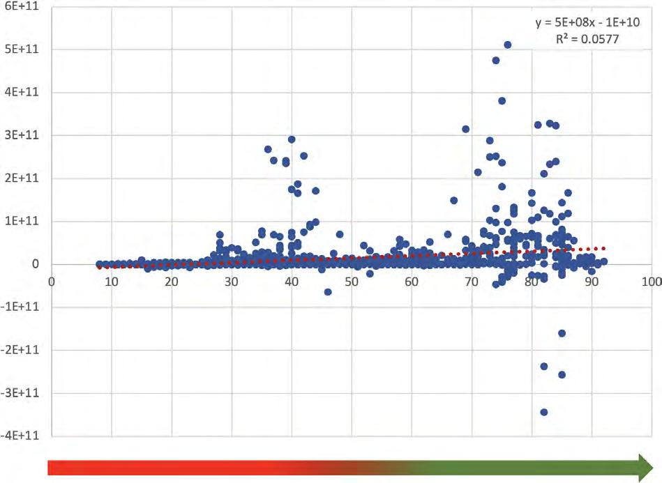
As can be seen below if we conduct a similar unrestrained analysis on net FDI flows, it shows not only a weak association between corruption and net flows, but also that the R-squared value of the data is particularly low.

Unlike the previous series, this report has not constrained the model (0 intercept). The rationale behind this is that economic activity could still occur (and so corruption is possible) within a country despite no net trade flows.

The outcome and conclusions

To better understand the relationship, in Appendix C we performed a similar analysis but for separate annual periods and it is interesting to note that the performance of other periods does vary considerably more than the GDP and industry value-added series.

2012, 2013 and 2014 have similar outcomes in terms of the slope of the relationship as do 2015, 2017 and 2020 and likewise for 2018 and 2019. Some of the explanation for this could be down to general economic conditions with improvements out of the financial crisis in the first period and some degree of normality in the mid period and then the entry into Covid for the later period.

Looking at the chart on the next page, it is reasonable to highlight that there are three areas where outliers over the various years are affecting this relationship. These are numbered one to three.

GDP and FDI flows – Unrestricted plot

1 3 4

2

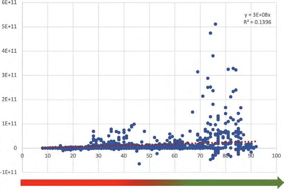
If we consider these areas, it could be argued that areas one and two (yellow) are distinct and could be considered outliers. Removing these from the results as shown below creates an improved R-squared, but it is fair to say the relationship between the CPI score and FDI net flows remains weak.

3

4

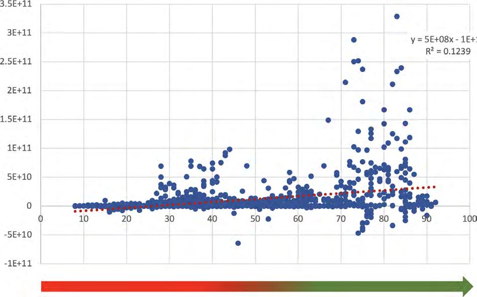
Then you could suggest that area 3 are also outliers (green) but unfortunately if this is removed as one would expect the slope of the relationship increases the R squared value actually falls.

4

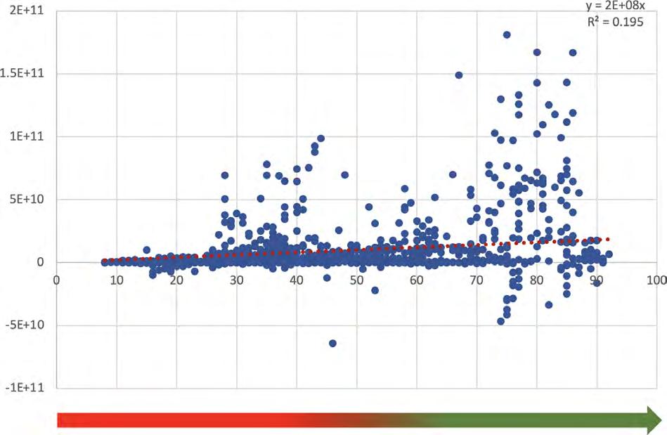
Finally, you could suggest that area 4 are also now outliers but as can be seen below this does further improve the R-squared value, suggesting a better fit with the data, but it also reduces the slope of the relationship between lower corruption and higher FDI flows.

At this stage of removal, it should rightly be questioned if it is reasonable to assume the result is still a fair reflection of the data. It is also important to note that the stepped approach taken in this report was done to demonstrate the difference such actions make, but also show potentially how the relationship changes.

So, what can we conclude from the stages and data as it has been analysed above?

• There is some relationship between FDI flows and corruption, with net FDI flows generally being higher in low corruption countries.

• Whilst net flows can be positive for a country, the extent to which flows occur depend on many factors and can be a political/economic decision.

• Whilst the relationship was not as strong as anticipated, the significant scale of the sums involved means even a small relationship results in significant loses.

• The relationship is, however, weak in terms of the amount of data that fits the linear relationship (R-squared value) unless you remove outliers.

• Having removed several stages of potential outliers, whilst the data fit improves, the relationship between corruption and net FDI gets weaker.

• Looking at the annual plots, unlike GDP per capita and value added in the industry (including construction), it is not as evident that the cost of corruption is increasing - ie: that the slope is increasing and so the benefit of reducing corruption is increasing.

Given all of the above results, this report next poses the question specifically for the industry – just what is the cost and implications of not reducing corruption?

A simple model - considering and calculating the cost of corruption over time and the extent to which reducing corruption makes a difference depending on its ‘cost’

One of the advantages of the analysis above is by also looking at individual year periods across countries, you are able to consider the potential cost of corruption in the light of the failure to act to prevent it.

Let’s consider that countries across the world had performed at the highest rate of Industry (including construction) value-added as opposed to the lowest. So, if corruption had the highest cost of growth verses the minimum, what would the result be?

As can be seen below, the linear slopes of the analysis of the lowest and highest year have been taken and the difference calculated. These are from the unconstrained model, taking the best case for the cost of corruption being significant (and having changed the most) and thus demonstrating the extent of change that needs to occur to tackle the cost of corruption faster.

The outcome and conclusions

The results show that a single point improvement in reducing corruption under the high versus low periods is $344 per person for industry value-added including construction. This was chosen to try and focus into the industry, infrastructure and construction sector.

Industry value-added (inc construction

Low slope gradient

1464.7

High slope gradient

1808.9

High low slope difference 344.2

As can be seen from Appendix D, using ILO data from the latest period on construction employmentxviii and the industry cost (which includes construction per point improvement) across the various countries where data is available, the difference in the cost of action of not reducing corruption by one point across each

employee would be approximately $38bn across the countries listed.

Consider then the latest CPI scores for 2021 and in a true drive to reduce corruption you raised all countries scores by ten, so no country was below 20 that is now worth $380bn in value-added lost in the industry

(including construction) sector.

You can easily see how even taking the different approach (which just considers the differential in corruption and not the totality of corruption within even the lower model, the cost of corruption if you were to raise all countries to a CPI score above 50, consider the cost of corruption and the cost of putting such activity right you would easily be hitting the $2.6tn cost of corruption per year (5% of GDP) mentioned by the UN using WEF data.xix

Our analysis, however, suggests that given the GDP per capita models were lower than the industry equivalent, the cost of this could be even higher. Whilst the simple approach that has been taken in this report is by no means definitive, it demonstrates the extreme cost of corruption, not only on economies and projects, but also on individuals across the globe.