14 minute read
CodeSport

by Hiba Dweib

CODE SPORT
Sandya Mannarswamy
Advertisement
In this month’s column, we continue our discussion on information retrieval.
Last month, I focused on the basic problem of information retrieval, namely, ‘ad-hoc information retrieval’ where, given a collection of documents, the user can arbitrarily query for any information which may or may not be contained in the given document collection. One of the well-known examples of ad-hoc information retrieval systems is the Web search engine, using which the user can pose a query on an arbitrary topic, and the set of documents is all the searchable Web pages available on the ‘World Wide Web’. A related but different kind of information retrieval is what is known as a ‘filtering’ task. In the case of filtering, a user profile is created, and a set of documents that may be of relevance or interest to the user are filtered from the document collection and presented to the user. A well-known example of information filtering is the personalisation of news delivery based on the user’s profile. Typically, in the case of the information filtering task, the set of documents in the document collection keeps changing dynamically (for instance, new news stories arrive and old news stories are retired from the collection), while the user query (for finding documents which are of interest based on the user profile) remains relatively stable. This is in contrast to ‘adhoc information retrieval’, wherein the document collection remains stable but queries keep changing dynamically.
In last month’s column, we discussed the Boolean model of ad-hoc information retrieval, wherein user information needs are presented in terms of a keyword-based query, and the documents in the collection are looked up using a Boolean model for the presence of the keywords in the query. For example, given that the document collection is the entire works of Shakespeare, the query term ‘Julius Caesar’ would find the documents that contain the query terms ‘Julius’ and ‘Caesar’ in them. In order to facilitate the queries, a data structure known as inverted index is generally built. The inverted index consists of the dictionary of terms in the document collection and a ‘pos list’ for each term, listing the document IDs which contain that term. Typically, the ‘pos list’ has not just the document IDs of the documents containing the term, but also contains the ‘position’ in the document where the term appears. Given the set of documents in the document collection, the pre-processing step is to construct the inverted index. So how do we construct this index? As I mentioned before, each document is scanned and broken into tokens or terms. There are two ways of constructing an inverted index. The first one is known as the ‘Blocked Sort Based Indexing’ (BSBI) method. Till now, when building inverted indexes was discussed, we made an implicit assumption that the data can fit in the main memory. But that assumption does not hold true for large document collections and, obviously, for a Web search. Hence, we need to consider the case when the document collection cannot be analysed in its entirety in the main memory to construct the inverted index. That’s where BSBI comes in.
BSBI divides the document collection into blocks, where each block can fit in the main memory. It then analyses one block, gets the terms in that block, and creates a sorted list of (term ID, doc ID) pairs. We can think of the sorting as being done with the ‘term ID’ as the primary key and the ‘doc ID’ as the secondary key. Note that since the block can fit in main memory, the sorting can be done in the main memory for that block and the results of the sorting are written back to the stable storage. Once all the blocks are processed, we have an ‘inverted index’ corresponding to each block of the document collection on disk in intermediate files. These intermediate ‘inverted indices’ need to be merged in order to construct the final ‘inverted index’ for the document collection. Let us assume that we have divided the document collection into 10 blocks. After the intermediate index construction step, we have 10 intermediate index files on disk. Now, in the final merging process, we open the 10 files, read data from each file into a read buffer, and we open a write buffer for writing back the results. During each step, we select the smallest term ID among those present in the read buffer and process it. All the document IDs corresponding to the term ID are processed and added to the ‘pos list’ for that term, and written back to disk. We can view this process as the equivalent of merging 10 individual sorted lists into one final sorted list. I leave it as an exercise for the reader to compute the complexity associated with BSBI.
Note that BSBI is a multi-pass algorithm since it breaks up the document collection into multiple blocks, processes each block individually in a sorting phase, and then merges the sorted results of each block in the final step. The alternative to BSBI is the ‘Single Pass In-Memory Indexing’ (SPIMI). While BSBI processes each block and creates a sorted list of (term ID, doc ID) pairs, SPIMI does not have the pre-processing step of creating the sorted list of (term ID, doc ID) pairs.
Similar to BSBI, SPIMI also divides the collection into blocks. But the division into blocks is governed by the memory available. As long as there is enough free memory available, SPIMI continues to process one term at a time. On encountering a term, SPIMI checks to see if the term is already encountered as part of the current block’s dictionary. If not, it creates a new term entry in the dictionary and creates a ‘pos list’ associated with that term. If the term is already present in the dictionary, it retrieves the ‘pos list’ associated with that term and adds this ‘doc ID’ to the ‘pos list’. When there is not enough free memory, it stops the processing of terms, sorts the current terms dictionary, writes it to disk and starts the processing of the next block. After processing all the terms, there are a number of on-disk block dictionaries which need to be combined to create the final ‘inverted index’.
Note that, till now, we have been discussing the creation of an inverted index for a document collection in a single computer system, and the only hardware constraint we have considered so far is the amount of available main memory in the computer system where the document collection is being processed. However, consider the case of constructing an inverted index for the document collection that comprises the ‘World Wide Web’. This task cannot be done on a single computer system and needs to be carried out on a very large cluster of machines. Hence, a distributed ‘inverted index’ creation method is needed. This is typically done in search engines using the ‘Map Reduce’ paradigm, which I will cover in my next column.
In the earlier discussion on BSBI and SPIMI, we assumed that documents can be scanned to get a token stream, and each token can be considered as a term for the document collection. Similarly, a user query is also broken down into query terms, and we look for documents which contain the query terms using the inverted index. We have glossed over many of the issues that arise when creating the terms from documents or queries. Documents can typically contain many common words such as ‘the’, ‘an’, ‘a’, etc. Such words do not contribute to deciding which documents are more relevant to a user query. Hence, such common terms need to be eliminated from being added to the term dictionary. This is typically achieved by what is known as a ‘stop word list’. Any word in the ‘stop word list’ is skipped from being processed when it is encountered in a document.
There are further complications in tokenisation. How do we handle hyphenated terms such as ‘anti-discriminatory’ or ‘wellknown’, etc? Do we break them into individual pieces or treat them as a single term? How do we handle the case sensitivity of terms in document collection and in queries? Case sensitivity can be useful in distinguishing between two semantically different query terms such as ‘Windows’ and ‘windows’. For instance, ‘Windows’ could potentially refer to the Windows operating system, whereas ‘windows’ could refer to windows in a house. But maintaining case sensitivity in an inverted index makes the index bloat up and, hence, most search engines/information retrieval systems do not support case sensitivity.
So far we have been considering simple queries where the user types the exact query without any spelling mistakes. But, frequently, users do misspell the query terms. Misspelled queries need to be handled intelligently by information retrieval systems such as search engines. We have often seen search engines give us intelligent hints such as, “Did you mean ‘carrot’?” when the user misspells ‘carrot’ as ‘carot’. One way of handling misspelled queries is to compute the edit distance from the misspelled word to words closest to it in the dictionary, and then use that set of words as the search term. Misspelled queries become more difficult to detect and deal with for proper nouns, such as in cases like ‘Tom Cruise’ getting misspelled as ‘Tom Cruse’, etc. The major challenge is to identify the subset of words in the dictionary for which we want to compute the edit distance with the query term.
Another challenge for information retrieval systems is the issue of handling wild card queries. I leave it as a take-away question to the reader to come up with an algorithm for handling wild card queries.
My ‘must-read book’ for this month
This month’s book suggestion comes from one of our readers, Nita Kumar. Her recommendation is the book, ‘Beautiful Data: The Stories Behind Elegant Data Solutions’ by Toby Segaran and Jeff Hammerbacher. It comprises a series of essays on elegant data solutions encompassing a wide spectrum of topics such as opinion polls data analysis, data analysis of Mars images and data storage on the cloud. By the way, Toby Segaran is the author of the famous book, ‘Programming the Collective Intelligence’, which discusses how to mine the data on the Web. Thank you, Nita for your recommendation.
If you have a favourite programming book/article that you think is a must-read for every programmer, please do send me a note with the book’s name, and a short write-up on why you think it is useful, so I can mention it in this column. This would help many readers who want to improve their software skills.
If you have any favourite programming questions/software topics that you would like to discuss on this forum, please send them to me, along with your solutions and feedback, at sandyasm_AT_yahoo_DOT_com. Till we meet again next month, happy programming!
By: Sandya Mannarswamy
The author is an expert in systems software and is currently working with Hewlett Packard India Ltd. Her interests include compilers, multi-core and storage systems. If you are preparing for systems software interviews, you may find it useful to visit Sandya's LinkedIn group Computer Science Interview Training India at http:// www.linkedin.com/groups?home=HYPERLINK "http://www. linkedin.com/groups?home=&gid=2339182"&HYPERLINK "http:// www.linkedin.com/groups?home=&gid=2339182"gid=2339182
Android Apps Made Easy with Processing

Any computer enthusiast would love to create an Android app, a seemingly difficult task. But combine Android with Processing and it is easy. Here’s a simple demonstration on how to use Android in tandem with Processing to create apps.
Android application development has become the coolest thing in the cyber world, for geeks and developers, and there is a great demand for them. Tutorials on Android app development with Eclipse can become frustrating at times. But as always, with the open source world, there is always an alternative way that works just out-of-the-box.
Android is a Linux-based operating system for mobile devices such as smartphones and tablet computers. It has been developed by the Open Handset Alliance, led by Google, and other companies. The initial developer of the software, Android Inc, was bought over by Google in 2005. The Android distribution was launched in 2007, and the Open Handset Alliance was founded. This is a consortium of 86 hardware, software and telecommunications companies devoted to advancing open standards for mobile devices. Google releases the Android code as open source, under the Apache License. The Android Open Source Project (AOSP) is tasked with the maintenance and further development of Android.
About Processing
Processing is an open source programming language and integrated development environment (IDE) built for the electronic arts and visual design communities with the purpose of teaching the basics of computer programming in a visual context, and to serve as the foundation for electronic sketchbooks. The project was initiated in 2001 by Casey Reas and Benjamin Fry. It brings complex graphics programming down to earth for the common man. For more, visit http:// www.processing.org
Before starting this tutorial I would like readers to get acquainted with Processing and its code, which is Java, and learn to write basic programs with it.
So combining Processing with Android can make the open source world livelier. Let’s look at how to develop Android apps using Processing and package them as .apk files.
Prerequisites
For this article I have used Processing 2.1 on Ubuntu 13.10. Processing can be downloaded from http://www.
processing.org/download/?processing Extract it to any folder of your choice. Download the Android SDK from: http://developer. android.com/sdk/index.html. Extract it where ever you like. Go into the extracted Android-SDK folder, into the tools subfolder and run android. In Linux, just open the terminal, cd to that folder and type ./android Through the GUI that launches, update and install all available packages. The main package is the Android SDK Platform-tools You can install the version of Android you want. Since I had a phone with Android 2.3, that is what I installed. Windows users need the Google USB drivers too. Once this is done, your system is ready to develop
Android apps.
Coding
On the terminal, cd to the folder in which you have extracted Processing and type ./processing. Make sure that the file Processing has the executable permission set. Start Processing. On the top right corner you will find a box called standard. Click on it and select android. Now write down the code. Most of the code in Processing can be used in Android, but there are certain exceptions. Here’s a small code example, in which we are creating an app to use a finger to draw on the smartphone screen.
void setup() { size(640,360); background(100); smooth(); stroke(255); } void draw() { if(mousePressed==true) { ellipse(mouseX,mouseY,5,5); } }
Press the Play button on the top left of the Processing window and wait till the emulator is loaded with the app. You can also connect your Android device to your PC and make the app run on your device. For that, you will have to activate the USB debugging mode in your Android device. Once you have tested your sketch and are satisfied, it is time to distribute it to the world and for that we have to package it.
Generating the .apk file
From the file menu in Processing, select Export
Android Project. A folder called Android is created in your sketch folder.
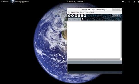
Figure 1: Android mode
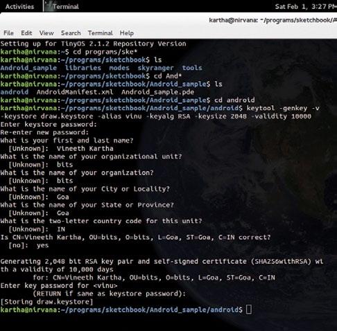
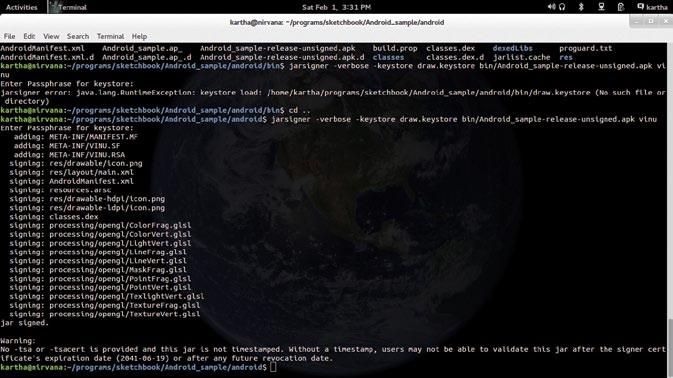
Figure 2: Generate the keystore
Open the terminal and cd to that particular folder. Then generate a private-public keypair, as follows:
$ keytool -genkey -v -keystore <keyfile.keystore> -alias <alias> -keyalg RSA -keysize 2048 -validity 10000
This command is nothing but generating a key and calling it draw.keystore. And it is valid for 10,000 days.
Answer all the questions which follow and remember those answers. Next, build the .apk:
$ ant release
This command will generate a file called sketchnamerelease-unsigned.apk in the bin folder. Sign the app:
$ jarsigner -verbose -keystore <Keyfile.keystore> bin/draw-
release-unsigned.apk <alias>
To execute this command, do remember to be in the directory in which your keyfile.keystore was located. Finally, generate the .apk file
For this, cd to the folder in which your Android SDK has been installed. Then cd to the Tools directory in AndroidSDK and type the following command:
$ ./zipalign -v 4 bin/sketchnamerelease-unsigned.apk name.apk
Your .apk file will be located in the tools folder as this is the location from Figure 3: Sign the .apk which you executed the zipalign command.
Wrapping it up
For more information, refer to http://wiki.processing. org/w/Android
This is how we step into the world of Android.
You now have your Android app ready for distribution to the world. In case you want your own icons, create icon-36.png, icon-48.png and icon-72.png. These should be 36×36, 48×48 and 72×72 pixel icons. Place them in the sketch folder (not the data folder or any other sub-folder), and rebuild the app.
By: Vineeth Kartha
The author is a post-graduate student in embedded systems at BITS Pilani, Goa. He has a great passion for open source technologies, computer programming and electronics. And when not coding, he loves to do glass paintings. He can be reached at vineeth.kartha@gmail.com or at http://www.thebeautifullmind.com