2 The light dawns

Chapter 2

The light dawns

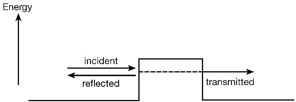
The years following Max Planck’s pioneering proposal were a time of confusion and darkness for the physics community. Light was waves; light was particles. Tantalizingly successful models, such as the Bohr atom, held out the promise that a new physical theory was in the offing, but the imperfect imposition of these quantum patches on the battered ruins of classical physics showed that more insight was needed before a consistent picture could emerge. When eventually the light did dawn, it did so with all the suddenness of a tropical sunrise.

In the years 1925 and 1926 modern quantum theory came into being fully fledged. These anni mirabiles remain an episode of great significance in the folk memory of the theoretical physics community, still recalled with awe despite the fact that living memory no longer has access to those heroic times. When there are contemporary stirrings in fundamental aspects of physical theory, people may be heard to say, ‘I have the feeling that it is 1925 all over again’. There is a wistful note present in such a remark. As Wordsworth said about the French Revolution, ‘Bliss it was in that dawn to be alive, but to be young was very heaven!’ In fact, though many important advances have been made in the last 75 years, there has not yet been a second time when radical revision of physical principles has been necessary on the scale that attended the birth of quantum theory.

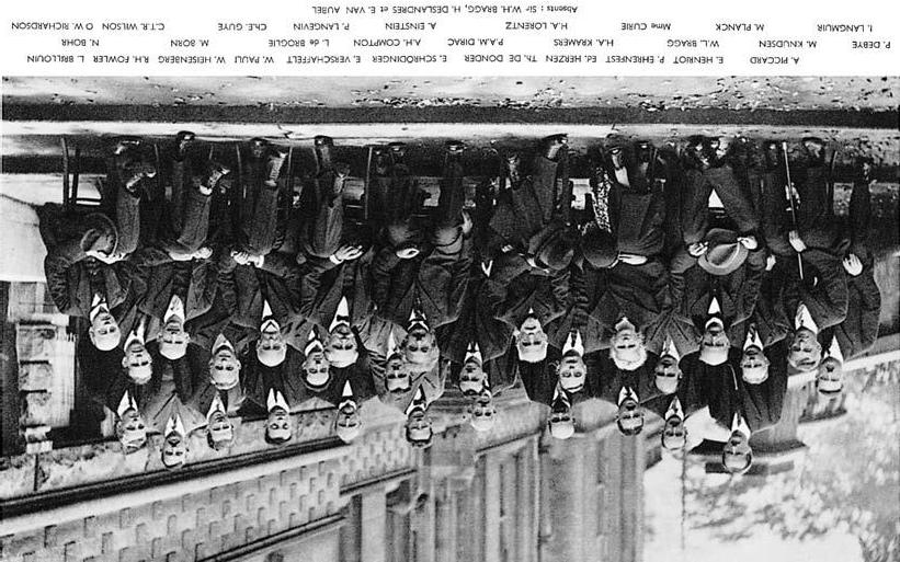
2.The great and the good of quantum theory: Solvay Conference 1927

Two men in particular set the quantum revolution underway, producing almost simultaneously startling new ideas.

Matrix mechanics

One of them was a young German theorist, Werner Heisenberg. He had been struggling to understand the details of atomic spectra. Spectroscopy has played a very important role in the development of modern physics. One reason has been that experimental techniques for the measurement of the frequencies of spectral lines are capable of great refinement, so that they yield very accurate results that pose very precise problems for theorists to attack. We have already seen a simple example of this in the case of the hydrogen spectrum, with Balmer’s formula and Bohr’s explanation of it in terms of his atomic model. Matters had become more complicated since then, and Heisenberg was concerned with a much wider and more ambitious assault on spectral properties generally. While recuperating on the North Sea island of Heligoland from a severe attack of hay fever, he made his big breakthrough. The calculations looked pretty complicated but, when the mathematical dust settled, it became apparent that what had been involved was the manipulation of mathematical entities called matrices (arrays of numbers that multiply together in a particular way). Hence Heisenberg’s discovery came to be known as matrix mechanics. The underlying ideas will reappear a little later in a yet more general form. For the present, let us just note that matrices differ from simple numbers in that, in general, they do not commute. That is to say, if A and B are two matrices, the product AB and the product BA are not usually the same. The order of multiplication matters, in contrast to numbers, where 2 times 3 and 3 times 2 are both 6. It turned out that this mathematical property of matrices has an important physical significance connected with what quantities could simultaneously be measured in quantum mechanics. [See 4 for a further mathematical generalization that proved necessary for the full development of quantum theory.]

In 1925 matrices were as mathematically exotic to the average theoretical physicist as they may be today to the average nonmathematical reader of this book. Much more familiar to the physicists of the time was the mathematics associated with wave motion (involving partial differential equations). This used techniques that were standard in classical physics of the kind that Maxwell had developed. Hard on the heels of Heisenberg’s discovery came a very different-looking version of quantum theory, based on the much more friendly mathematics of wave equations.

Wave mechanics

Appropriately enough, this second account of quantum theory was called wave mechanics. Although its fully developed version was discovered by the Austrian physicist Erwin Schrödinger, a move in the right direction had been made a little earlier in the work of a young French aristocrat, Prince Louis de Broglie [5]. The latter made the bold suggestion that if undulating light also showed particlelike properties, perhaps correspondingly one should expect particles such as electrons to manifest wavelike properties. De Broglie could cast this idea into a quantitative form by generalizing the Planck formula. The latter had made the particlelike property of energy proportional to the wavelike property of frequency. De Broglie suggested that another particlelike property, momentum (a significant physical quantity, well-defined and roughly corresponding to the quantity of persistent motion possessed by a particle), should analogously be related to another wavelike property, wavelength, with Planck’s universal constant again the relevant constant of proportionality. These equivalences provided a kind of mini-dictionary for translating from particles to waves, and vice versa. In 1924, de Broglie laid out these ideas in his doctoral dissertation. The authorities at the University of Paris felt pretty suspicious of such heterodox notions, but fortunately they consulted Einstein on the side. He recognized the young man’s genius and the degree was awarded. Within a few years, experiments by Davisson and Germer in the United States, and by

George Thomson in England, were able to demonstrate the existence of interference patterns when a beam of electrons interacted with a crystal lattice, thereby confirming that electrons did indeed manifest wavelike behaviour. Louis de Broglie was awarded the Nobel Prize for physics in 1929. (George Thomson was the son of J. J. Thomson. It has often been remarked that the father won his Nobel Prize for showing that the electron is a particle, while the son won his Nobel Prize for showing that the electron is a wave.)

The ideas that de Broglie had developed were based on discussing the properties of freely moving particles. To attain a full dynamical theory, a further generalization would be required that allowed the incorporation of interactions into its account. This is the problem that Schrödinger succeeded in solving. Early in 1926 he published the famous equation that now goes by his name [6]. He had been led to its discovery by exploiting an analogy drawn from optics.

Although physicists in the 19th century thought of light as consisting of waves, they did not always use the full-blown calculational techniques of wave motion to work out what was happening. If the wavelength of the light was small compared to the dimensions defining the problem, it was possible to employ an altogether simpler method. This was the approach of geometrical optics, which treated light as moving in straight line rays which were reflected or refracted according to simple rules. School physics calculations of elementary lens and mirror systems are performed today in just the same fashion, without the calculators having to worry at all about the complexities of a wave equation. The simplicity of ray optics applied to light is similar to the simplicity of drawing trajectories in particle mechanics. If the latter were to prove to be only an approximation to an underlying wave mechanics, Schrödinger argued that this wave mechanics might be discoverable by reversing the kind of considerations that had led from wave optics to geometrical optics. In this way he discovered the Schrödinger equation.

Schrödinger published his ideas only a few months after Heisenberg had presented his theory of matrix mechanics to the physics community. At the time, Schrödinger was 38, providing an outstanding counterexample to the assertion, sometimes made by non-scientists, that theoretical physicists do their really original work before they are 25. The Schrödinger equation is the fundamental dynamical equation of quantum theory. It is a fairly straightforward type of partial differential equation, of a kind that was familiar to physicists at that time and for which they possessed a formidable battery of mathematical solution techniques. It was much easier to use than Heisenberg’s new-fangled matrix methods. At once people could set to work applying these ideas to a variety of specific physical problems. Schrödinger himself was able to derive from his equation the Balmer formula for the hydrogen spectrum. This calculation showed both how near and yet how far from the truth Bohr had been in the inspired tinkering of the old quantum theory. (Angular momentum was important, but not exactly in the way that Bohr had proposed.)

Quantum mechanics

It was clear that Heisenberg and Schrödinger had made impressive advances. Yet at first sight the way in which they had presented their new ideas appeared so different that it was not clear whether they had made the same discovery, differently expressed, or whether there were two rival proposals on the table [see the discussion of 10]. Important clarificatory work immediately followed, to which Max Born in Göttingen and Paul Dirac in Cambridge were particularly significant contributors. It soon became established that there was a single theory that was based on common general principles, whose mathematical articulation could take a variety of equivalent forms. These general principles were eventually most transparently set out in Dirac’s Principles of Quantum Mechanics, first published in 1930 and one of the intellectual classics of the 20th century. The preface to the first edition begins with the deceptively simple statement, ‘The methods of progress in

theoretical physics have undergone a vast change during the present century’. We must now consider the transformed picture of the nature of the physical world that this vast change had introduced.

I learned my quantum mechanics straight from the horse’s mouth, so to speak. That is to say, I attended the famous course of lectures on quantum theory that Dirac gave in Cambridge over a period of more than 30 years. The audience included not only final year undergraduates like myself, but frequently also senior visitors who rightly thought it would be a privilege to hear again the story, however familiar it might be to them in outline, from the lips of the man who had been one of its outstanding protagonists. The lectures followed closely the pattern of Dirac’s book. An impressive feature was an utter lack of emphasis on the part of the lecturer on what had been his own considerable personal contribution to these great discoveries. I have already spoken of Dirac as a kind of scientific saint, in the purity of his mind and the singleness of his purpose. The lectures enthralled one by their clarity and the majestic unfolding of their argument, as satisfying and seemingly inevitable as the development of a Bach fugue. They were wholly free from rhetorical tricks of any kind, but near the beginning Dirac did permit himself a mildly theatrical gesture.

He took a piece of chalk and broke it in two. Placing one fragment on one side of his lectern and the other on the other side, Dirac said that classically there is a state where the piece of chalk is ‘here’ and one where the piece of chalk is ‘there’, and these are the only two possibilities. Replace the chalk, however, by an electron and in the quantum world there are not only states of ‘here’ and ‘there’ but also a whole host of other states that are mixtures of these possibilities – a bit of ‘here’ and a bit of ‘there’ added together. Quantum theory permits the mixing together of states that classically would be mutually exclusive of each other. It is this counterintuitive possibility of addition that marks off the quantum

world from the everyday world of classical physics [7]. In professional jargon this new possibility is called the superposition principle.

Double slits and superposition

The radical consequences that follow from the assumption of superposition are well illustrated by what is called the double slits experiment. Richard Feynman, the spirited Nobel Prize physicist who has caught the popular imagination by his anecdotal books, once described this phenomenon as lying at ‘the heart of quantum mechanics’. He took the view that you had to swallow quantum theory whole, without worrying about the taste or whether you could digest it. This could be done by gulping down the double slits experiment, for

In reality it contains the only mystery. We cannot make the mystery go away by ‘explaining’ how it works. We will just tell you how it works. In telling you how it works we will have told you about the basic peculiarities of all quantum mechanics.

After such a trailer, the reader will surely want to get to grips with this intriguing phenomenon. The experiment involves a source of quantum entities, let us say an electron gun that fires a steady stream of particles. These particles impinge on a screen in which there are two slits, A and B. Beyond the slitted screen there is a detector screen that can register the arrival of the electrons. It could be a large photographic plate on which each incident electron will make a mark. The rate of delivery from the electron gun is adjusted so that there is only a single electron traversing the apparatus at any one time. We then observe what happens.

The electrons arrive at the detector screen one by one, and for each of them one sees a corresponding mark appearing that records its point of impact. This manifests individual electron behaviour in a particlelike mode. However, when a large number of marks have

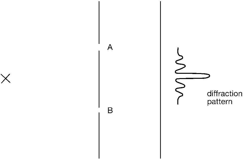
3.The double slits experiment

accumulated on the detector screen, we find that the collective pattern they have created shows the familiar form of an interference effect. There is an intense dark spot on the screen opposite the point midway between the two slits, corresponding to the location where the largest number of electron marks have been deposited. On either side of this central band there are alternating light and diminishingly dark bands, corresponding to the non-arrival and arrival of electrons at these positions respectively. Such a diffraction pattern (as the physicists call these interference effects) is the unmistakable signature of electrons behaving in a wavelike mode.

The phenomenon is a neat example of electron wave/particle duality. Electrons arriving one by one is particlelike behaviour; the resulting collective interference pattern is wavelike behaviour. But there is something much more interesting than that to be said. We can probe a little deeper into what is going on by asking the question, When an indivisible single electron is traversing the apparatus, through which slit does it pass in order to get to the detector screen? Let us suppose that it went through the top slit,

A. If that were the case, the lower slit B was really irrelevant and it might just as well have been temporarily closed up. But, with only A open, the electron would not be most likely to arrive at the midpoint of the far screen, but instead it would be most likely to end up at the point opposite A. Since this is not the case, we conclude that the electron could not have gone through A. Standing the argument on its head, we conclude that the electron could not have gone through B either. What then was happening? That great and good man, Sherlock Holmes, was fond of saying that when you have eliminated the impossible, whatever remains must have been the case, however improbable it may seem to be. Applying this Holmesian principle leads us to the conclusion that the indivisible electron went through both slits. In terms of classical intuition this is a nonsense conclusion. In terms of quantum theory’s superposition principle, however, it makes perfect sense. The state of motion of the electron was the addition of the states (going through A) and (going through B).

The superposition principle implies two very general features of quantum theory. One is that it is no longer possible to form a clear picture of what is happening in the course of physical process. Living as we do in the (classical) everyday world, it is impossible for us to visualize an indivisible particle going through both slits. The other consequence is that it is no longer possible to predict exactly what will happen when we make an observation. Suppose we were to modify the double slits experiment by putting a detector near each of the two slits, so that it could be determined which slit an electron had passed through. It turns out that this modification of the experiment would bring about two consequences. One is that sometimes the electron would be detected near slit A and sometimes it would be detected near slit B. It would be impossible to predict where it would be found on any particular occasion but, over a long series of trials, the relative probabilities associated with the two slits would be 50–50. This illustrates the general feature that in quantum theory predictions of the results of measurement

are statistical in character and not deterministic. Quantum theory deals in probabilities rather than certainties. The other consequence of this modification of the experiment would be the destruction of the interference pattern on the final screen. No longer would electrons tend to the middle point of the detector screen but they would split evenly between those arriving opposite A and those arriving opposite B. In other words, the behaviour one finds depends upon what one chooses to look for. Asking a particlelike question (which slit?) gives a particlelike answer; asking a wavelike question (only about the final accumulated pattern on the detector screen) gives a wavelike answer.

Probabilities

It was Max Born at Göttingen who first clearly emphasized the probabilistic character of quantum theory, an achievement for which he would only receive his well-deserved Nobel Prize as late as 1954. The advent of wave mechanics had raised the familiar question, Waves of what? Initially there was some disposition to suppose that it might be a question of waves of matter, so that it was the electron itself that was spread out in this wavelike way. Born soon realized that this idea did not work. It could not accommodate particlelike properties. Instead it was waves of probability that the Schrödinger equation described. This development did not please all the pioneers, for many retained strongly the deterministic instincts of classical physics. Both de Broglie and Schrödinger became disillusioned with quantum physics when presented with its probabilistic character.

The probability interpretation implied that measurements must be occasions of instantaneous and discontinuous change. If an electron was in a state with probability spread out ‘here’, ‘there’, and, perhaps, ‘everywhere’, when its position was measured and found to be, on this occasion, ‘here’, then the probability distribution had suddenly to change, becoming concentrated solely on the actually measured position, ‘here’. Since the probability distribution is to

be calculated from the wavefunction, this too must change discontinuously, a behaviour that the Schrödinger equation itself did not imply. This phenomenon of sudden change, called the collapse of the wavepacket, was an extra condition that had to be imposed upon the theory from without. We shall see in the next chapter that the process of measurement continues to give rise to perplexities about how to understand and interpret quantum theory. In someone like Schrödinger, the issue evoked more than perplexity. It filled him with distaste and he said that if he had known that his ideas would have led to this ‘damn quantum jumping’ he would not have wished to discover his equation!

Observables

(Warning to the reader: This section includes some simple mathematical ideas that are well worth the effort to acquire, but whose digestion will require some concentration. This is the only section in the main text to risk a glancing encounter with mathematics. I regret that it cannot help being somewhat hardgoing for the non-mathematician.)

Classical physics describes a world that is clear and determinate. Quantum physics describes a world that is cloudy and fitful. In terms of the formalism (the mathematical expression of the theory), we have seen that these properties arise from the fact that the quantum superposition principle permits the mixing together of states that classically would be strictly immiscible. This simple principle of counterintuitive additivity finds a natural form of mathematical expression in terms of what are called vector spaces [7].

A vector in ordinary space can be thought of as an arrow, something of given length pointing in a given direction. Arrows can be added together simply by following one after the other. For example, four miles in a northerly direction followed by three miles in an easterly direction adds up to five miles in a direction 37° east of north (see

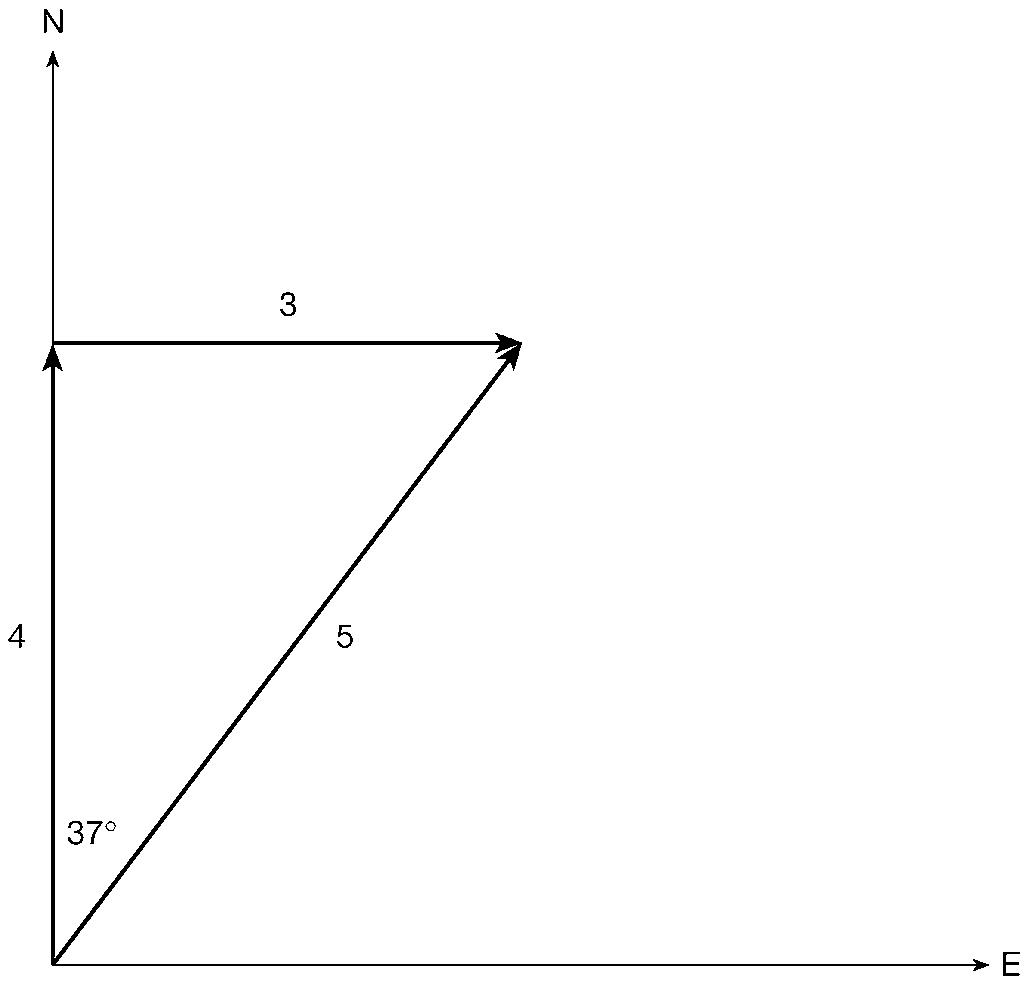
4.Adding vectors

figure 4). Mathematicians can generalize these ideas to spaces of any number of dimensions. The essential property that all vectors have is that they can be added together. Thus they provide a natural mathematical counterpart to the quantum superposition principle. The details need not concern us here but, since it is always good to feel at home with terminology, it is worth remarking that a particularly sophisticated form of vector space, called a Hilbert space, provides the mathematical vehicle of choice for quantum theory.

So far the discussion has concentrated on states of motion. One may think of them as arising from specific ways of preparing the initial material for an experiment: firing electrons from an electron gun; passing light through a particular optical system; deflecting

particles by a particular set of electric and magnetic fields; and so on. One can think of the state as being ‘what is the case’ for the system that has been prepared, though the unpicturability of quantum theory means that this will not be as clear and straightforward a matter as it would be in classical physics. If the physicist wants to know something more precisely (where actually is the electron?), it will be necessary to make an observation, involving an experimental intervention on the system. For example, the experimenter may wish to measure some particular dynamical quantity, such as the position or the momentum of an electron. The formal question then arises: If the state is represented by a vector, how are the observables that can be measured to be represented? The answer lies in terms of operators acting on the Hilbert space. Thus the scheme linking mathematical formalism to physics includes not only the specification that vectors correspond to states, but also that operators correspond to observables [8].

The general idea of an operator is that it is something that transforms one state into another. A simple example is provided by rotation operators. In ordinary three-dimensional space, a rotation through 90° about the vertical (in the sense of a right-handed screw) turns a vector (think of it as an arrow) pointing east into a vector (arrow) pointing north. An important property of operators is that usually they do not commute with each other; that is to say the order in which they act is significant. Consider two operators: R1, a rotation through 90° about the vertical; R2, a rotation through 90° (again right-handed) about a horizontal axis pointing north. Apply them in the order R1 followed by R2 to an arrow pointing east. R1 turns this into an arrow pointing north, which is then unchanged by R2. We represent the two operations performed in this order as the product R2.R1, since operators, like Hebrew and Arabic, are always read from right to left. Applying the operators in the reverse order first changes the eastward arrow into an arrow pointing downwards (effect of R2), which is then left unchanged (effect of R1). Since R2.R1 ends up with an arrow pointing north and R1.R2

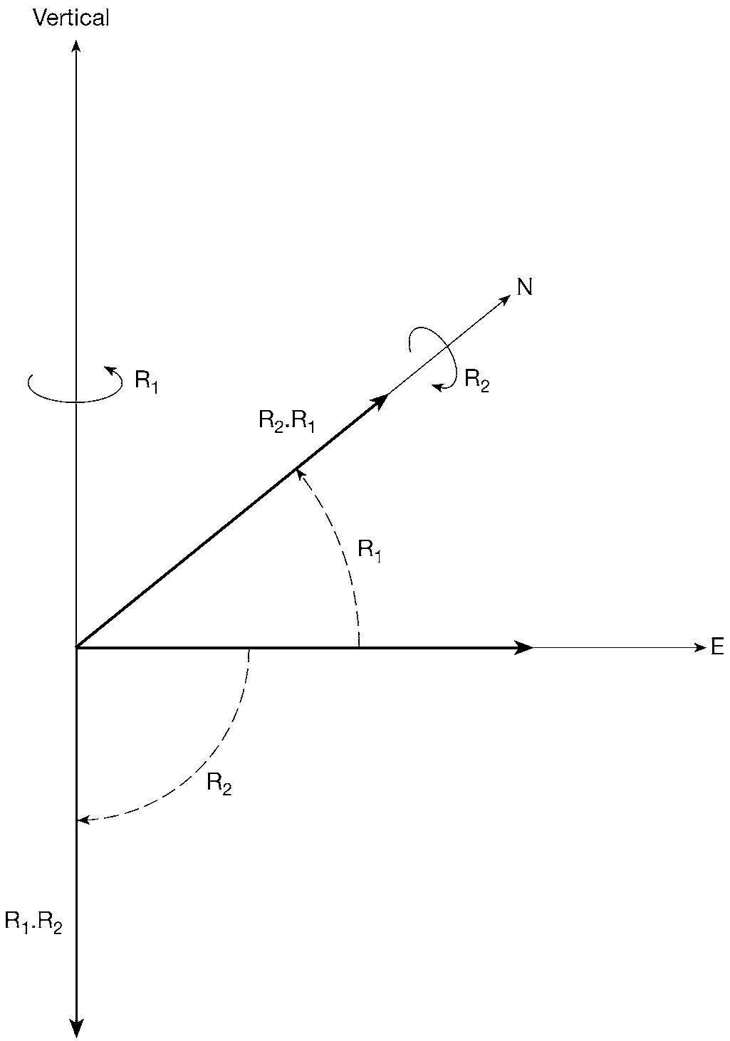
5.Non-commuting rotations

ends up with an arrow pointing downwards, these two products are quite distinct from each other. The order matters – rotations do not commute.

Mathematicians will recognize that matrices can also be considered as operators, and so the non-commutativity of the matrices that Heisenberg used is another specific example of this general operator property.

All this may seem pretty abstract, but non-commutativity proves to be the mathematical counterpart of an important physical property. To see how this comes about, one must first establish how the operator formalism for observables is related to the actual results of experiments. Operators are fairly sophisticated mathematical entities, but measurements are always expressed as unsophisticated numbers, such as 2.7 units of whatever it might be. If abstract theory is to make sense of physical observations, there must be a way of associating numbers (the results of observations) with operators (the mathematical formalism). Fortunately mathematics proves equal to this challenge. The key ideas are eigenvectors and eigenvalues [8].

Sometimes an operator acting on a vector does not change that vector’s direction. An example would be a rotation about the vertical axis, which leaves a vertical vector completely unchanged. Another example would be the operation of stretching in the vertical direction. This would not change a vertical vector’s direction, but it would change its length. If the stretch has a doubling effect, the length of the vertical vector gets multiplied by 2. In more general terms, we say that if an operator O turns a particular vector v into a multiple λ of itself, then v is an eigenvector of O with eigenvalue λ. The essential idea is that eigenvalues (λ) give a mathematical way of associating numbers with a particular operator (O) and a particular state (v). The general principles of quantum theory include the bold requirement that an eigenvector (also called an eigenstate) will correspond physically to a state in

A number of significant consequences flow from this rule. One is the converse, that, because there are many vectors that are not eigenvectors, there will be many states in which measuring O will not give any particular result with certainty. (Mathematica aside: it is fairly easy to see that superposing two eigenstates of O corresponding to different eigenvalues will give a state that cannot be a simple eigenstate of O.) Measuring O in states of this latter kind must, therefore, give a variety of different answers on different occasions of measurement. (The familiar probabilistic character of quantum theory is again being manifested.) Whatever result is actually obtained, the consequent state must then correspond to it; that is to say, the vector must change instantaneously to become the appropriate eigenvector of O. This is the sophisticated version of the collapse of the wavepacket.

Another important consequence relates to what measurements can be mutually compatible, that is to say, made at the same time. Suppose it is possible to measure both O1 and O2 simultaneously, with results λ1 and λ2, respectively. Doing so in one order multiplies the state vector by λ1 and then by λ2, while reversing the order of the observations simply reverses the order in which the λs multiplies the state vector. Since the λs are just ordinary numbers, this order does not matter. This implies that O2.O1 and O1.O2 acting on the state vector have identical effects, so that the operator order does not matter. In other words, simultaneous measurements can only be mutually compatible for observables corresponding to operators that commute with each other. Putting it the other way round, observables that do not commute will not be simultaneously measurable.

Here we see the familar cloudiness of quantum theory being manifested again. In classical physics the experimenter can measure whatever is desired whenever it is desired to do so. The

physical world is laid out before the potentially all-seeing eye of the scientist. In the quantum world, by contrast, the physicist’s vision is partially veiled. Our access to knowledge of quantum entities is epistemologically more limited than classical physics had supposed.

Our mathematical flirtation with vector spaces is at an end. Any reader who is dazed should simply hold on to the fact that in quantum theory only observables whose operators commute with each other can be measured simultaneously.

The uncertainty principle

What all this means was considerably clarified by Heisenberg in 1927 when he formulated his celebrated uncertainty principle. He realized that the theory should specify what it permitted to be known by way of measurement. Heisenberg’s concern was not with mathematical arguments of the kind that we have just been considering, but with idealized ‘thought experiments’ that sought to explore the physical content of quantum mechanics. One of these thought experiments involved considering the so-called γ-ray microscope.

The idea is to find out in principle how accurately one might be able to measure the position and momentum of an electron. According to the rules of quantum mechanics, the corresponding operators do not commute. Therefore, if the theory really works, it should not be possible to know the values of both position and momentum with arbitrary accuracy. Heisenberg wanted to understand in physical terms why this was so. Let’s start by trying to measure the electron’s position. In principle, one way to do this would be to shine light on the electron and then look through a microscope to see where it is. (Remember these are thought experiments.) Now, optical instruments have a limited resolving power, which places restrictions on how accurately objects can be located. One cannot do better than the wavelength of the light being used. Of course one way to increase accuracy would be to use shorter wavelengths –

which is where the γ-rays come in, since they are very highfrequency (short wavelength) radiation. However, this ruse exacts a cost, resulting from the particlelike character of the radiation. For the electron to be seen at all, it must deflect at least one photon into the microscope. Planck’s formula implies that the higher the frequency, the more energy that photon will be carrying. As a result, decreasing the wavelength subjects the electron to more and more by way of an uncontrollable disturbance of its motion through its collision with the photon. The implication is that one increasingly loses knowledge of what the electron’s momentum will be after the position measurement. There is an inescapable trade-off between the increasing accuracy of position measurement and the decreasing accuracy of knowledge of momentum. This fact is the basis of the uncertainty principle: it is not possible simultaneously to have perfect knowledge of both position and momentum [9]. In more picturesque language, one can know where an electron is, but not know what it is doing; or one can know what it is doing, but not know where it is. In the quantum world, what the classical physicist would regard as half-knowledge is the best that we can manage.

This demi-knowledge is a quantum characteristic. Observables come in pairs that epistemologically exclude each other. An everyday example of this behaviour can be given in musical terms. It is not possible both to assign a precise instant to when a note was sounded and to know precisely what its pitch was. This is because determining the pitch of a note requires analysing the frequency of the sound and this requires listening to a note for a period lasting several oscillations before an accurate estimate can be made. It is the wave nature of sound that imposes this restriction, and if the measurement questions of quantum theory are discussed from the point of view of wave mechanics, exactly similar considerations lead back to the uncertainty principle.

There is an interesting human story behind Heisenberg’s discovery. At the time he was working at the Institute in Copenhagen, whose head was Niels Bohr. Bohr loved interminable discussions and the

young Heisenberg was one of his favourite conversation partners. In fact, after a while, Bohr’s endless ruminations drove his younger colleague almost to distraction. Heisenberg was glad to seize the opportunity afforded by Bohr’s absence on a skiing holiday to get on with his own work by completing his paper on the uncertainty principle. He then rushed it off for publication before the grand old man got back. When Bohr returned, however, he detected an error that Heisenberg had made. Fortunately the error was correctable and doing so did not affect the final result. This minor blunder involved a mistake about the resolving power of optical instruments. It so happened that Heisenberg had had trouble with this subject before. He did his doctoral work in Munich under the direction of Arnold Sommerfeld, one of the leading protagonists of the old quantum theory. Brilliant as a theorist, Heisenberg had not bothered much with the experimental work that was also supposed to be a part of his studies. Sommerfeld’s experimental colleague, Wilhelm Wien, had noted this. He resented the young man’s cavalier attitude and decided to put him through it at the oral examination. He stumped Heisenberg precisely with a demand to derive the resolving power of optical instruments! After the exam, Wien asserted that this lapse meant that Heisenberg should fail. Sommerfeld, of course (and rightly), argued for a pass at the highest level. In the end, there had to be a compromise and the future Nobel Prize winner was awarded his PhD, but at the lowest possible level.

Probability amplitudes

The way in which probabilities are calculated in quantum theory is in terms of what are called probability amplitudes. A full discussion would be inappropriately mathematically demanding, but there are two aspects of what is involved of which the reader should be aware. One is that these amplitudes are complex numbers, that is to say, they involve not only ordinary numbers but also i, the ‘imaginary’ square root of −1. In fact, complex numbers are endemic in the formalism of quantum theory. This is because they afford a very convenient way of representing an aspect of waves that was referred

to in Chapter 1, in the course of discussing interference phenomena. We saw that the phase of waves relates to whether two sets of waves are in step or out of step with each other (or any possibility intermediate between these two). Mathematically, complex numbers provide a natural and convenient way of expressing these ‘phase relations’. The theory has to be careful, however, to ensure that the results of observations (eigenvalues) are free from any contamination by terms involving i. This is achieved by requiring that the operators corresponding to observables satisfy a certain condition that the mathematicians call being ‘hermitean’ [8].

The second aspect of probability amplitudes that we need at least to be told about is that, as part of the mathematical apparatus of the theory that we have been discussing, their calculation is found to involve a combination of state vectors and observable operators. Since it is these ‘matrix elements’ (as such combinations are called) that carry the most direct physical significance, and because it turns out that they are formed from what one might call state-observable ‘sandwiches’, the time-dependence of the physics can be attributed either to a time-dependence present in the state vectors or to a time-dependence present in the observables. This observation turns out to provide the clue to how, despite their apparent differences, the theories of Heisenberg and Schrödinger do actually correspond to exactly the same physics [10]. Their seeming dissimilarity arises from Heisenberg’s attributing all the timedependence to the operators and Schrödinger’s attributing it wholly to the state vectors.

The probabilities themselves, which to make sense must be positive numbers, are calculated from the amplitudes by a kind of squaring (called ‘the square of the modulus’) that always yields a positive number from the complex amplitude. There is also a scaling condition (called ‘normalization’) that ensures that when all the probabilities are added together they total up to 1 (certainly something must happen!).

All the while these wonderful discoveries were coming to light, Copenhagen had been the centre where assessments were made and verdicts delivered on what was happening. By this time, Niels Bohr was no longer himself making detailed contributions to technical advances. Yet he remained deeply interested in interpretative issues and he was the person to whose integrity and discernment the Young Turks, who were actually writing the pioneering papers, submitted their discoveries. Copenhagen was the court of the philosopher-king, to whom the intellectual offerings of the new breed of quantum mechanics were brought for evaluation and recognition.

In addition to this role as father-figure, Bohr did offer an insightful gloss on the new quantum theory. This took the form of his notion of complementarity. Quantum theory offered a number of alternative modes of thought. There were the alternative representations of process that could be based on measuring either all positions or all momenta; the duality between thinking of entities in terms of waves or in terms of particles. Bohr emphasized that both members of these pairs of alternatives were to be taken equally seriously, and could be so treated without contradiction because each complemented rather than conflicted with the other. This was because they corresponded to different, and mutually incompatible, experimental arrangements that could not both be employed at the same time. Either you set up a wave experiment (double slits), in which case a wavelike question was being asked that would receive a wavelike answer (an interference pattern); or you set up a particle experiment (detecting which slit the electron went through) in which case the particlelike question received a particlelike answer (two areas of impact opposite the two slits).

Complementarity was obviously a helpful idea, though it by no means resolved all interpretative problems, as the next chapter will show. As Bohr grew older he became increasingly concerned with

philosophical issues. He was undoubtedly a very great physicist, but it seems to me that he was distinctly less gifted at this later avocation. His thoughts were extensive and cloudy, and many books have subsequently been written attempting to analyse them, with conclusions that have assigned to Bohr a variety of mutually incompatible philosophical positions. Perhaps he would not have been surprised at this, for he liked to say that there was a complementarity between being able to say something clearly and its being something deep and worth saying. Certainly, the relevance of complementarity to quantum theory (where the issue arises from experience and we possess an overall theoretical framework that renders it intelligible) provides no licence for the easy export of the notion to other disciplines, as if it could be invoked to ‘justify’ any paradoxical pairing that took one’s fancy. Bohr may be thought to have got perilously close to this when he suggested that complementarity could shed light on the age-old question of determinism and free will in relation to human nature. We shall postpone further philosophical reflection until the final chapter.

Quantum logic

One might well expect quantum theory to modify in striking ways our conceptions of such physical terms as position and momentum. It is altogether more surprising that it has also affected how we think about those little logical words ‘and’ and ‘or’.

Classical logic, as conceived of by Aristotle and the man on the Clapham omnibus, is based on the distributive law of logic. If I tell you that Bill has red hair and he is either at home or at the pub, you will expect either to find a red-haired Bill at home or a red-haired Bill at the pub. It seems a pretty harmless conclusion to draw, and formally it depends upon the Aristotelian law of the excluded middle: there is no middle term between ‘at home’ and ‘not at home’. In the 1930s, people began to realize that matters were different in the quantum world. An electron can not only be ‘here’ and ‘not here’, but also in any number of other states that are

superpositions of ‘here’ and ‘not here’. That constitutes a middle term undreamed of by Aristotle. The consequence is that there is a special form of logic, called quantum logic, whose details were worked out by Garret Birkhoff and John von Neumann. It is sometimes called three-valued logic, because in addition to ‘true’ and ‘false’ it countenances the probabilistic answer ‘maybe’, an idea that philosophers have toyed with independently.