25 minute read
I(x,y) /(F(x,y) *I(x,y
International Journal of Artificial Intelligence and Applications (IJAIA), Vol.12, No.2, March 2021
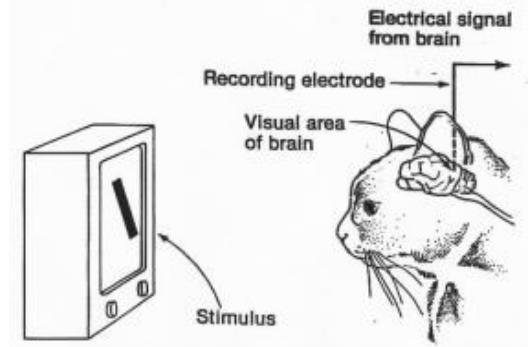
were activated, when exhibited to vertical edges and also another set of neurons fired when exposed to horizontal or diagonal edges. All of these categories of neurons are arranged in a columnar configuration and collectively these neurons can produce visual perception.
Advertisement
Different portions of the visual cortex are classified as V1, V2, V3, and V4. In general, V1 and V2 regions of visual cortex are having close resemblance with convolutional and subsampling layers, whereas inferior temporal region resembles the higher layers of CNN [16]. During theprocess of training, CNN learns with the help of backpropagation algorithm by making adjustments in weights with respect to the target.
Fig.2. Hubel and Wiesel experiment
3.2. CNN Architecture
In CNN architecture, network layers are divided into three types: the convolutional, pooling and fully connected layers [20]. The architecture of CNN is as shown in Fig 3.
3.2.1. Convolutional Layer
In CNN, every neuron in the convolutional layer is linked only to a small portion of the neurons in the preceding layer, which is in square shape area across the height and width dimensions. The size of this square is a hyperparameter (controllable parameter) and called as Receptive Field. For the depth dimension, there is no hyperparameter available since the convolution operations are normally carried out for the whole depth. Generally, the depth dimension of the input describes the various colors of the image. Hence it is usually required to link them in order to bring out necessary information.
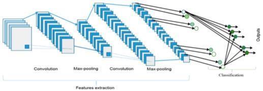
Fig.3.The CNN architecture
6
International Journal of Artificial Intelligence and Applications (IJAIA), Vol.12, No.2, March 2021
Neurons present in the convolution operator can recognize certain local patterns of the previous layer’s output. Once features are obtained, its actual position is not important and all the neurons are expected to identify the same pattern. This is achieved by forcing all the neurons to have a common single set of parameters known as Parameter Sharing [9].
In order to identify various unique features within one layer, it is necessary to have multiple filters, where each filter is a group of neurons that recognize a certain pattern at different locations in the image.
3.2.2. Pooling Layer
The main aim of pooling layer is to reduce the complexity of CNNs. The neurons present in the pooling layer form a square shaped area across the width and height dimensions of the preceding layer. Even though it is very similar to the convolutional layer, it is different from convolutional layer because the pooling layer is Non-Parametrized Layer.
The function carried out by this layer is known as subsampling or down sampling. During this process, contraction in size results in concurrent loss of data. On the other hand, such a loss is helpful to the network because the reduction in size not only reduces the computational burden for the succeeding layers of the network and also it reduces the effects of overfitting [12].
Max pooling and average pooling are the generally used techniques shown in (Fig.4). Max Pooling chooses the largest element within each receptive field [14] whereas Average Pooling computes the average among the output neurons within the pooling window. Max-pooling chooses the most prominent feature in a pooling window. On the other hand, average-pooling method selects whole features into consideration. Thus, max-pooling method keeps texture related information, while average pooling method retains the background related data [24]. Pooling operation does not combine neurons with different depth values. Instead, the resulting pooling layer will have the uniform depth as the previous layer and it will only combine local areas within a filter.
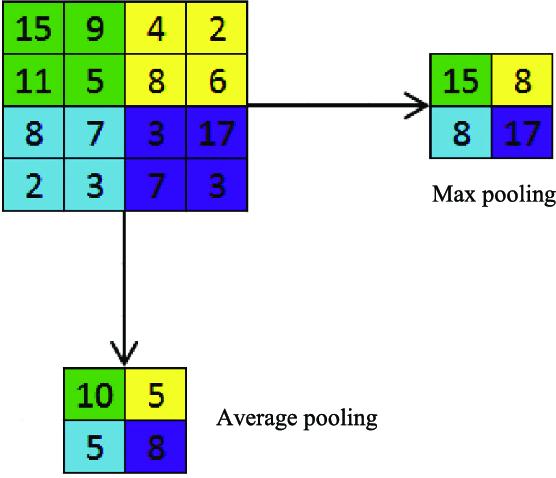
Fig.4.Max Pooling and Average Pooling Operations Illustration.
3.2.3. Fully Connected Layer
The filters and neurons present in this layer are connected to all the activation in the preceding layers resulting in a completely connected structure. Hence the name. The output feature maps of the final convolution or pooling layer is converted into a one-dimensional (1D) array of numbers [18]. High-level reasoning in the network is carried out via fully connected layers [19].
7
International Journal of Artificial Intelligence and Applications (IJAIA), Vol.12, No.2, March 2021
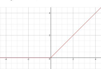
The final fully connected layer has the same number of output nodes as the number of classes. Each fully connected layer is followed by a nonlinear function, such as ReLU (Rectified Linear Units). ReLU is an activation function operates by thresholding values at 0, i.e. f (x) = max (0, x). In other words, it outputs 0 when x < 0, and contrarily, it outputs a linear function with a slope of 1 when x ≥ 0 [15] as shown in the (Fig.5).
3.3. CNN Operation
Fig.5. The Rectified Linear Unit (ReLU)
Based on local receptive field, each component in a convolutional layer accepts inputs from a set of adjacent units belonging to the preceding layer layer. This way neurons are proficient in extracting rudimentary features like edges or corners. These features are then linked by the succeeding convolutional layers in order to further extract high level features.
The components of a convolutional layer are arranged in planes. All units of a plane share the same set of weights. Thus, each plane is in charge for building a particular feature. The results obtained from the plane is termed as feature maps. Each convolutional layer consists of several planes, so that multiple feature maps can be constructed at each location. The most significant features derived are passed from initial layers to higher layers. As the features are passed to the higher layer, there is a dimensionality reduction in features determined by kernel size of the convolutional and max-pooling layers. On the other hand, there is an increase in number of feature maps for representing better features of the input images for ensuring classification accuracy [13]. The derived feature vector either could be an input for classification task or could be treated as a feature vector for next level processing.
The network designed to do the classification task consists of several convolution pooling layers followed by some fully-connected layers. The first two layers mentioned above perform convolution and pooling operation in order to extract high-level features. The final layer’s output of CNN is applied as the input to a fully connected network, which does the task of classification. The output layer for classification task consists of one neuron for each class and the values of these neurons describes the score of each class. If score distribution is chosen, the score range will be between zero and one. The summation of class scores is one. The values of each neuron can be presumed as the probability of occurrence of the class.
8
International Journal of Artificial Intelligence and Applications (IJAIA), Vol.12, No.2, March 2021
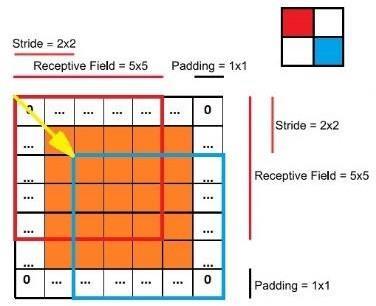
Fig.6. A visual representation of the various hyperparameters of convolutional layers: receptive field, stride and padding
4. EXPERIMENTAL SETUP
The implementations are carried out in MATLAB 2019b on a workstation with windows 10 OS, AMD processor with 2.0 GHz, hard drive with 8 GB RAM. The experiments are conducted in Extended Yale B and FERET Database with deep CNN model.
4.1. Extended Yale B Database
The extended Yale Face Database B contains 16128 images of 28 human subjects under 9 poses and 64 illumination conditions as shown in (Fig.7). The data format of this database is the same as that of the Yale Face Database B.
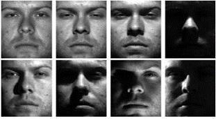
Fig.7. Images from extended Yale B database.
4.2. FERET Database
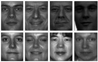
The FERET database was collected in 15 sessions between August 1993 and July 1996. The database contains 1564 sets of images for a total of 14,126 images that includes 1199 individuals and 365 duplicate sets of images as shown in (Fig.8). A duplicate set is a second set of images of a person already in the database and was usually taken on a different day.
9
International Journal of Artificial Intelligence and Applications (IJAIA), Vol.12, No.2, March 2021
4.3. Experiment
Fig.8. Images from FERET database
The model uses a deep CNN network with six convolution layers (with size 3x3), two maxpooling and two fully convolutional layers. The first two convolutions use 8 filters, next two uses 16 and the last convolution layers uses 32 each in order to extract complex features.
The model uses batch normalization and dropouts in all convolutional layers along with ReLU activation function. In order to reduce the overfitting, the dropout rate is kept higher on the final convolutional layers. Two maxpooling layers are introduced after second and fourth convolutional layers to reduce the feature space dimension. The two fully connected layers use 128 and 28 neurons respectively. The final classification layer uses softmax activation with categorical cross entropy loss function. The softmax layer is used to produce the classification scores, in which each score is the probability of a particular class for a given instance [31].
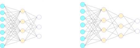
The dropout principle is employed on the convolutional neural networks model and the value of drop out is chosen by trial and error method. The (Fig.9) shows the network model with drop out and the values of the drop out is different for different layers. The model also uses Adam
Optimizer with a learning rate of 0.001 which was found empirically after trying different combinations.
The feature maps are subsampled with maxpooling layers with a stride of 2x2. Stride is the number of pixels which shifts over the input matrix. When the stride is 2, it means the filter is moved by 2 pixels at a time. The number of neurons in this output layer is limited to 28 in Extended Yale B database. In FERET database, the number of neurons in the output layer is 994.
Data Augmentation is implemented in the form of simple methods like resizing, rotation, and reflection. The batch size of 128 and number of epochs 250 are chosen to achieve best results.
The training is designed to use different batch sizes to do a fair trade off between accuracy and training time.
(a) (b)
Fig.9. (a) The neural networks model (b) The model after applying drop out
10
International Journal of Artificial Intelligence and Applications (IJAIA), Vol.12, No.2, March 2021
5. RESULTS
The CNN trained with back-propagation algorithm in batch mode with a various batch sizes of 4, 8, 16 and 32 for different epochs are computed for Extended YALE B with an image size of 128×128 for 50 epochs. The same experiment is conducted on FERET database for the frontal face image size of 128×128 for 300 epochs.
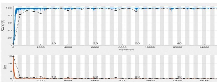
For the Extended YALE B Database, the maximum accuracy rate of 97.2% is achieved for the batch size of 4 without applying preprocessing technique as shown in (Fig.10). After applying the preprocessing techniques, the maximum accuracy is improved to 99.8% as shown in (Fig.11).
For the batch size of 8, the maximum accuracy rate of 97.0% is achieved without applying any preprocessing technique. After applying the preprocessing techniques, the maximum accuracy is improved to 99.4%.
For the batch size of 8, SQI, LTISN and HE perform very equally well and yield the maximum accuracy of 99.4%, 99.3% and 99.1%.
For the batch size of 16, the maximum accuracy rate of 96.8% is achieved without applying preprocessing technique. After applying the preprocessing techniques, the maximum accuracy is improved to 99.1%.
For the batch size of 16 HE, SQI and GIC perform equally well and yield the maximum accuracy of 99.1%. 98.8% and 98.8% respectively.
For the batch size of 32, the maximum accuracy rate of 96.2% is achieved without applying preprocessing technique. After applying the preprocessing techniques, the maximum accuracy is improved to 98.7% for the same batch size.
For the batch size of 32, GIC, SQI, and HE perform equally well and yield the maximum accuracy of 98.7%, 98.3% and 98.3% respectively. Table 1 shows the accuracy rates of Extended Yale B database for various batch sizes before and after application of preprocessing techniques.
For the FERET Database, the maximum accuracy rate of 71.4% is achieved without applying preprocessing technique, for the batch size of 4, as shown in (Fig.12). After applying the preprocessing techniques, the maximum accuracy improved to 76.6% as shown in (Fig.13).
DoG, HE and LTISN perform equally well and yield the maximum accuracy of 76.6%, 76.3% and 75.6% respectively.
For the batch size of 8, the maximum accuracy rate of 71.2% is achieved without applying preprocessing technique. After applying the preprocessing techniques, the maximum accuracy is improved to 76.4%.
For the batch size of 8, HE, SQI and LTISN perform very equally well and yield the maximum accuracy of 76.4%, 74.6% and 72.5% respectively.
For the batch size of 16, the maximum accuracy rate of 71.0% is achieved without applying preprocessing technique. After applying the preprocessing techniques, the maximum accuracy is improved to 76.1%.
11
International Journal of Artificial Intelligence and Applications (IJAIA), Vol.12, No.2, March 2021
For the batch size of 16 HE, LTISN and SQI perform very equally well and yield the maximum accuracy of 76.1%, 72.0% and 71.5% respectively.
For the batch size of 32, the maximum accuracy rate of 68.7% is achieved without applying preprocessing technique. After applying the preprocessing techniques, the maximum accuracy is improved to 71.0%.
For the batch size of 32, SQI, GIC, LTISN and DoG perform equally well and yield the maximum accuracy of 71%, 70.9%, 70.8% and 69.9% respectively.
SQI and HE perform equally well and provide best results for all the batch sizes in both Extended Yale B and FERET database.
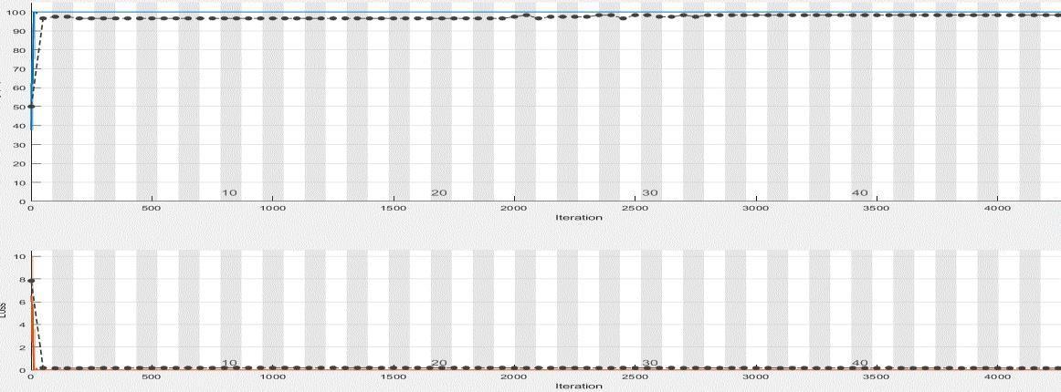
Fig.10.Accuracy using Extended YALE B Database before applying of preprocessing techniques
Fig.11.Accuracy using Extended YALE B Database after application of preprocessing techniques
12
International Journal of Artificial Intelligence and Applications (IJAIA), Vol.12, No.2, March 2021

Fig.12.Accuracy using FERET Database before the application of preprocessing techniques.

Fig.13.Accuracy using FERET Database after application of preprocessing techniques.

Table 1 Accuracy rates of Extended Yale B database for various batch sizes before and after application of preprocessing techniques.
Database Accuracy Rates Batch Size 4 8 16 32
Extended Yale B (WOAPP) 97.2 97.0 96.8 96.2 DoG 99.1 99.0 98.7 97.9 SQI 99.8 99.4 98.8 98.3 LTISN 99.2 99.3 98.4 98.1 HE 99.7 99.1 99.1 98.3 GIC 99.6 98.9 98.8 98.7
13
International Journal of Artificial Intelligence and Applications (IJAIA), Vol.12, No.2, March 2021 Table 2 Accuracy rates of FERET database for various batch sizes before and after application of preprocessing techniques
Database AccuracyRates Batch Size 4 8 16 32
FERET(WOAPP) 71.4 71.2 71 68.7 DoG 76.6 72.6 71.3 69.9 SQI 74.9 74.6 71.5 71.0 LTISN 75.6 72.5 72.0 70.8 HE 76.3 76.4 76.1 69.2 GIC 74.2 71.3 71.0 70,9
Data augmentation with the batch size of 128 and number of epochs 250 yields best results, especially with the preprocessing technique Histogram Equalization. In FERET Database, the maximum accuracy of 79.6% is achieved.
For the same batch size and number of epochs, LTISN provides almost the same accuracy rate of 78.9%.
DoG, SQI and GIC performs almost equally and provides the accuracy enhancement of 78.2%, 78.3% and 78.1%
Data augmentation Methods does not have much effect in Extended Yale B database. With the batch size of 128 and number of epochs 250 yields best results, especially with the preprocessing technique of Histogram Equalization. In Extended Yale B Database, the maximum accuracy of 99.86% is achieved.
For the same batch size and number of epochs, SQI and LTISN provides almost the same accuracy rate of 99.91% and 99.31%
DoG, HE and GIC performs almost equally and provides the accuracy enhancement of 99.21%, 99.78% and 99.71%
The number of trainable parameters is computed for each layer as below. The deep architecture is as shown in (Fig.14).
C1 Layer
Input image 128×128×1 and having one channel. Number of weights per filter=3×3×1 There are totally eight filters in C1 layer and there is one bias parameter for each filter.
Total number of trainable parameters in C1 Layer is = (3×3×1+1) × 8= 80.
C2 Layer
Input feature maps to C2 layer having 8 channels. Number of weights per filter is 3×3×8.
14
International Journal of Artificial Intelligence and Applications (IJAIA), Vol.12, No.2, March 2021
There are 8 such filters in the layer. Hence total number of weights = ((3×3×8) +1) ×8 and ther e is one bias for each filter. Total weights in C2 = ((3×3×8) +1) ×12=584.
S1 Layer
S1 layer is using max pooling operation. Hence no trainable parameter available for this layer.
C3 Layer
Input to C3 has eight feature channels. Number of weights per filter is 3×3×8. There are 16 such filters in the layer. Hence total number of weights = ((3×3) ×8+1) ×16 and there is one bias for each filter. Total weights in C3 = (3×3×8+1) ×16=1168.
C4 Layer
Input to C4 has sixteen feature channels. Number of weights per filter is 3×3×16. There are 16 such filters in the layer. Hence total number of weights = ((3×3) ×16+1) ×16 and there is one bias for each filter. Total weights in C4 = (3×3×16+1) ×16=2320.
S2 Layer
S2 layer is using max pooling operation. Hence no trainable parameter available for this layer.
C5 Layer
Input to C5 has sixteen feature channels. Number of weights per filter is 3×3×16. There are 32 such filters in the layer. Hence total number of weights = ((3×3) ×16+1) ×32 and there is one bias for each filter. Total weights in C4 = (3×3×16+1) ×32=4640.
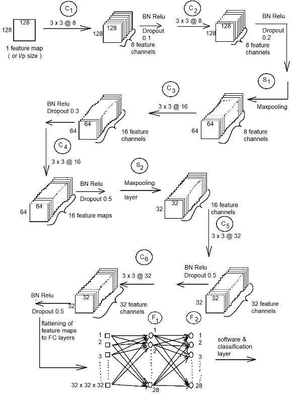
Fig.14. Deep CNN Model Architecture (BN-Batch Normalization)
15
International Journal of Artificial Intelligence and Applications (IJAIA), Vol.12, No.2, March 2021
C6 Layer
Input to C6 has 32 feature channels. Number of weights per filter is 3×3×32 There are 32 such filters in the layer. Hence total number of weights = (3×3 ×32+1) ×32 and there is one bias for each filter. Total weights in C4 = (3×3×32+1) ×32=9248.
F1 Layer
In the fully connected layer, the input is having total feature space of size 32×32 and 32. Input samples to F1 layer=32×32×32 There are 128 neurons in F1 layer and each have a bias. Total Number of trainable parameters for F1 layer is = (32×32×2+1) ×128=4194432.
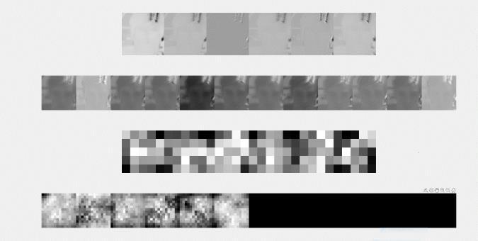
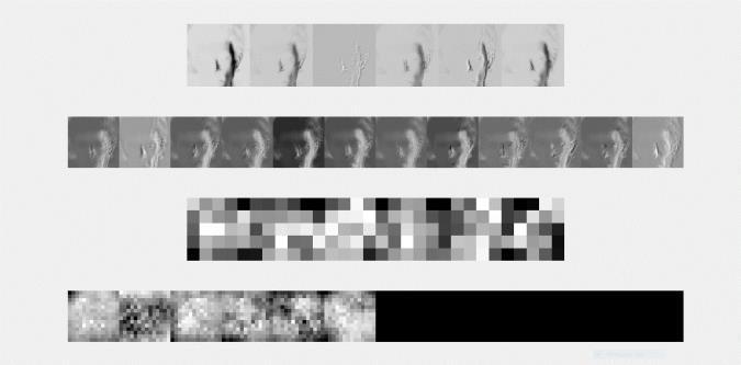
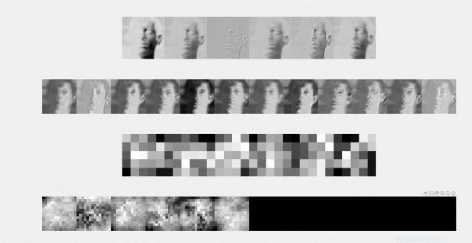
Fig.15.Feature map obtained for the batch size 32 and epoch 2
Fig.16.Feature map obtained for the batch size 32 and epoch 5
Fig.17.Feature map obtained for the batch size 32 and epoch 25
16
International Journal of Artificial Intelligence and Applications (IJAIA), Vol.12, No.2, March 2021
F2 Layer
The input to F2 layer is the output from F1 layer. It is connected to 28 neurons (since there are 28 classes). So, total number of trainable parameters = (128 +1) ×28= 16512. Feature maps extracted for different batch size and epochs are as shown in the (Fig.15,16,17).
6. COMPARISON WITH OTHER APPROACHES
In this section, the proposed approach is compared with the various approaches.
Hybrid system, which combines convolutional neural network (CNN) and a Logistic regression classifier (LRC) yields the accuracy of 80%. A CNN is trained to recognize facial images and LRC is used to classify the features learned by the convolutional network [26]. The neural network with the nonlinear theories, such as wavelet theory and fuzzy set is a new research idea, when applied in face recognition, gives accuracy around 93% in Wavelet-BP [25]. CNN architecture along with Max-Feature-Map (MFM) could extract compact vital information yields the accuracy rate of 98% [28]. The popular LeNet-5 architecture in FERET database yields accuracy rate is 81.25% [27]. The pre-trained CNN model along with the VGG- Face provides face verification rate accuracy of 86.85% and 83.32% on FRGC and LFW databases respectively [29].
Table 3. Comparison of Accuracy rates of different approaches.
Sno Architectureused Dataset Accuracy 1 Proposedmethod(C Extended Yale 99.8% NN) BFERET 76.3% 2 VGG+CNN[29] FRGC,LFW 86.85%, 83.32%
3 CNN withMAF activationfunction [28] LFW 98%
4 Wavelet-BP[25] AT&T 93.0% 5 CNN-LRC Yale 80% [26] 6 CNN-LENET[27] FERET 81.25%
The proposed method compared with existing approaches are given in Table 3. The proposed method performs better in comparison to all other approaches in Extended Yale B. In FERET database, CNN-LENET method performs better than the proposed method.
7. CONCLUSION
In this paper, deep convolution neural network (CNN) is applied for extracting features and classification. The performance of the network is assessed before and after applying preprocessing techniques for various batch sizes and epochs on YALE B and FERET dataset.
Adam optimizers with a learning rate of 0.001 is applied in this experiment. The batch sizes used in this experiment are [4, 8, 16,32];
The optimum batch sizes are chosen using trial and error method. Initially, multiple batch sizes of [4,8,16,32,64,128] are selected for this experiment. Batch size of 4 with learning rate of0.001 and
17
International Journal of Artificial Intelligence and Applications (IJAIA), Vol.12, No.2, March 2021
number of epochs 50 give the best results. Batch sizes of [4,8,16,32] provide consistent and best results. The batch sizes are normally selected in power of 2. Choosing smaller batch size with low value of learning rate yields best result.
The results showed the maximum accuracy rate of 97.2% of achieved without using preprocessing techniques. When the preprocessing techniques are applied, the improved accuracy rates are achieved up to 99.8%.
The same experiments are conducted in FERET. dataset also. For the frontal face, the maximum 71.4% is achieved without optimization. After applying the preprocessing techniques, the accuracy rate increased to 76.3%.
The proposed approach performs very well as compared to existing methods.
REFERENCES
[1] S. Setiowati, Zulfanahri, E. L. Franita and I. Ardiyanto, "A review of optimization method in face recognition: Comparison deep learning and non-deep learning methods” 9th International Conference on Information Technology and Electrical Engineering (ICITEE), Phuket, pp. 1-6, 2017. [2] Aleix M. Marttinez and Avinash C. Kak, “PCA versus LDA”. IEEE Transactions on Pattern Analysis and Machine Intelligence, Vol. 23, No.2, pp. 228-233, 2001. [3] Rahul Haridas, Jyothi R L “Convolutional Neural Networks: A Comprehensive Survey” International
Journal of Applied Engineering Research Volume 14, Number 3, pp. 780-789, (2019). [4] Goodfellow, I. J., Bengio, Y., and Courville, A. Deep Learning MIT Press, (2016). [5] Jason Wang, Luis Perez The Effectiveness of Data Augmentation in Image Classification using Deep
Learning. In: Stanford University research report, 2017. [6] Di Huang, Caifeng Shan, Mohsen Ardebilian, Yunhong Wang, and Liming Chen “Local Binary
Patterns and Its Application to Facial Image Analysis: A Survey” IEEE Transactions on Systems,
Man and Cybernetics, part C, volume 41, pp 765-781, 2011. [7] Shailaja A Patil and Dr. P. J. Deore “Face Recognition: A Survey” Informatics Engineering, an
International Journal (IEIJ), Vol.1, No.1, December 2013. [8] Connor Shorten and Taghi M. Khoshgoftaar “A survey on Image Data Augmentation for Deep
Learning” Jounal of Big Data, - Springer, 2019. [9] Felix Ellenberger, Claus Lenz “A Non-Technical Survey on Deep Convolutional
Neural Network Architectures” Computer Vision and Pattern Recognition, 2018. [10] S.V.G. Reddy, K. Thammi Reddy, V. ValliKumari “Optimization of Deep Learning using various
Optimizers, Loss functions and Dropout” International Journal of Recent Technology and
Engineering (IJRTE) Volume-7 Issue-4S2, pp 448-455, December 2018. [11] SaezTrigueros, D.; Meng, L.; Hartnett, M. Face Recognition: From Traditional to Deep Learning
Methods. J. Theory. Appl. Inf. Technol. 2018, 97, 3332–3342. [12] Athanasios Voulodimos, Nikolaos Doulamis, AnastasiosDoulamis, and EftychiosProtopapadakis
“Deep Learning for Computer Vision: A Brief Review” Computational Intelligence and
Neuroscience, pp 1-13, 2018. [13] MdZahangirAlom, Tarek M. Taha, Chris Yakopcic, Stefan Westberg, PahedingSidike,
MstShamimaNasrin, Mahmudul Hasan, Brian C. van Essen, Abdul A. S. Awwal and Vijayan K.
Asari “A State-of-the-Art Survey on Deep Learning Theory and Architectures”. Electronics 2019, 8, 292 [14] WaseemRawat and Zenghui Wang “Deep Convolutional Neural Networks for Image Classification:
A Comprehensive Review” Volume 29, pp 2352-2449 September 2017. [15] A. F. Agarap. Deep learning using rectified linear units (relu). CoRR, abs/1803.08375, URL http://arxiv.org/abs/1803.08375 , 2018. [16] Khan, Asifullah&Sohail, Anabia&Zahoora, Umme& Saeed, Aqsa “A Survey of the Recent
Architectures of Deep Convolutional Neural Networks”, published in Artificial Intelligence Review (2019).
18
International Journal of Artificial Intelligence and Applications (IJAIA), Vol.12, No.2, March 2021 [17] D. H. Hubel and T. N. Wiesel. “Receptive fields of single neurons in the cat’s striate cortex” The
Journal of Physiology, 148(3):574–91, 1959. [18] Yamashita, R., Nishio, M., Do, R.K.G. et al. “Convolutional neural networks: an overview and application in radiology” Insights Imaging 9, pp 611–629, 2018. [19] MamounAlazab, MingJian Tang “Deep Learning Applications for Cyber Security”, Springer, ISBN 978-3- 030-13057-2, May 2019. [20] N. Aloysius and M. Geetha, "A review on deep convolutional neural networks," 2017 International
Conference on Communication and Signal Processing (ICCSP), Chennai, pp. 0588-0592, doi: 10.1109/ICCSP.2017.8286426, 2017. [21] Nusrat, Ismoilov and Sung-Bong Jang. “A Comparison of Regularization Techniques in Deep Neural
Networks.” Symmetry 10 (2018): 648. [22] B. S. Manjunath, R. Chellappa and C. von der Malsburg, "A feature-based approach to face recognition," Proceedings 1992 IEEE Computer Society Conference on Computer Vision and Pattern
Recognition, Champaign, IL, USA, pp. 373-378, 1992. [23] Srivastava, Nitish et al. “Dropout: a simple way to prevent neural networks from overfitting.” J.
Mach. Learn. Res. 15, pp 1929-1958, (2014). [24] Zhao, Qi et al. “Multiactivation Pooling Method in Convolutional Neural Networks for Image
Recognition.” Wireless Communications and Mobile Computing (2018): n. page. Wireless
Communications and Mobile Computing. Web, 2018. [25] J. Kittler, P. Koppen, et. al, "Conformal Mapping of a 3D Face Representation onto a 2D Image for
CNN Based Face Recognition," 2018 International Conference on Biometrics (ICB), Gold Coast,
QLD, pp. 124-131, 2018. [26] H. Khalajzadeh, M. Manthouri and M. Teshnehlab, ’Face recognition using convolutional neural networks and simple logistic classifier’, Advances in intelligent systems and computing, 223, pp 197207, (2014). [27] A.R. syafeeza, M.K. Hani, S.S. Uiw and R. Bakhteri,’ Convolutional neural network for face recognition with pose and illumination variation’, International journal of engineering and
Technology, 6(1), pp 44-57, (2014). [28] Y. Xu, F. Liang, G. Zhang and H. Xu, ‘Image intelligent detection based on the Gabor wavelet and the neural network’, Symmetry, 8(130), (2016). [29] Wu, Xiang et al. “A Lightened CNN for Deep Face Representation.” ArXiv abs/1511.02683 (2015):n. pag. [30] Z. Lu, X. Jiang and A. Kot, "Enhance deep learning performance in face recognition,” 2nd
International Conference on Image, Vision and Computing (ICIVC), Chengdu, pp. 244-248, 2017. [31] Pouyanfar, S., Sadiq, S., Yan, Y., Tian, H., Tao, Y., Reyes, M. P, Iyengar, S. S. A survey on deep learning: Algorithms, techniques, and applications. ACM Computing Surveys, 51(5), (2018). [32] Y. Admi, Y. Moses and S. Ulman “Face Recognition: The problem of compensating for changes in illumination direction”, IEEE Transaction. Pattern Anal. Mach. Intell., vol. 19, pp 721–732, Jul. 1997. [33] SoodehNikan and M. Ahmadi. “Human Face Recognition under Occlusion using LBP and Entropy
Weighted Voting” 21st International Conference on Pattern Recognition ICPR pp. 1699-1702, 2012. [34] S. Anila, K. Arulsukanya, K. Divya, C. Kanimozhi, and D. Kavitha “An efficient Preprocessing
Technique for Face Recognition under difficult Lighting Conditions,” in Proc. National Conference on Emerging Trends in Computer Communication and Informatics (ETCCI-2011), March 10-11, 2011. [35] Hu Han, Shiguang Shan, Xilin Chen, Wen Gao “A comparative study on illumination preprocessing in face recognition” Pattern Recognition., Volume 46, Issue 6, Pages 1691-1699, June 2013. [36] Calvo G., Baruque B., Corchado E. (2013) Study of the Pre-processing Impact in a Facial
Recognition System. In: Pan JS., Polycarpou M.M., Woźniak M., de Carvalho A.C.P.L.F., Quintián
H., Corchado E. (eds) Hybrid Artificial Intelligent Systems. HAIS, Lecture Notes in Computer
Science, vol 8073. Springer, Berlin, Heidelberg, 2013. [37] Koringa P.A., Mitra S.K., Asari, V.K. Handling Illumination Variation: A Challenge for Face
Recognition. In: Raman B., Kumar S., Roy P., Sen D. (eds) Proceedings of International Conference on Computer Vision and Image Processing. Advances in Intelligent Systems and Computing, vol 460.
Springer, Singapore, 2017.
19
International Journal of Artificial Intelligence and Applications (IJAIA), Vol.12, No.2, March 2021 [38] Dr. A. Sri Krishna, G. Srinivasa Rao and M. Sravya “Contrast Enhancement Techniques using
Histogram Equalization Methods on Color Images with Poor Lightning”, International Journal of
Computer Science, Engineering and Applications (IJCSEA) Vol.3, No.4, August 2013. [39] P. Suganya, S. Gayathri, N. Mohanapriya “Survey on Image Enhancement Techniques” International
Journal of Computer Applications Technology and Research, Volume 2– Issue 5, 623 - 627, 2013. [40] Biglari M, Mirzaei F, Ebrahimpour-Komeh H. Illumination invariant face recognition using SQI and weighted LBP histogram[C]. Pattern Recognition and Image Analysis (PRIA), 2013 First Iranian
Conference on. IEEE, pp 1-7, 2013. [41] E Krieger, VK Asari, and S Arigela. Color image enhancement of low-resolution images captured in extreme lighting conditions. In SPIE Sensing Technology and Applications, pages 91200Q– 91200Q.
International Society for Optics and Photonics, 2014. [42] Anila, S., and N. Devarajan. "Preprocessing technique for face recognition applications under varying illumination conditions." Global Journal of Computer Science and Technology Volume 12, issue 11,
Version 1, 2012. [43] NungsanginlaLongkumer, Mukesh Kumar and RohiniSaxena “Contrast Enhancement Techniques using Histogram Equalization: A Survey” International Journal of Current Engineering and
Technology, Vol.4, No.3, E-ISSN 2277 – 4106, P-ISSN 2347 – 5161 (June 2014). [44] Ali M. Reza. "Realization of the Contrast Limited Adaptive Histogram Equalization (CLAHE) for
Real-Time Image Enhancement." Journal of VLSI Signal Processing, vol. 38, pp 35-44, 2004. [45] Porcu, S.; Floris, A.; Atzori, L. Evaluation of Data Augmentation Techniques for Facial Expression
Recognition Systems. Electronics 2020, 9, 1892. https://doi.org/10.3390/electronics9111892. [46] Zagoruyko, K. Wide residual networks. In BMVC, 2016. [47] DeVries, T. and Taylor, G. W. Improved regularization of convolutional neural networks with cutout. arXiv preprint arXiv:1708.04552, 2017. [48] Y. Bengio, A. Bergeron, N. Boulanger-Lewandowski, T. Breuel, Y. Chherawala, et al. Deep learners benefit more from out-of-distribution examples. In Proceedings of the Fourteenth International
Conference on Artificial Intelligence and Statistics, pages 164–172, 2011. [49] R. Wu, S. Yan, Y. Shan, Q. Dang, and G. Sun. Deep image: Scaling up image recognition. arXiv preprint arXiv:1501.02876, 7(8), 2015.
20


