Back Propagation

Dr. Deepa A1 , Fathima Thasliya P A2

1Associate professor, Department of MCA, Nehru college of Engineering and Research Centre, Thrissur

2Department of MCA, Nehru College of Engineering and Research Centre, Trissur

Abstract: Back Propagation Algorithm research is now very active in the Artificial Neural Network (ANN) and machine learning communities. It has increased a wide range of applications, including image compression, pattern recognition, time series prediction, sequence identification, data filtering, and other intelligent processes carried out by the human brain, have had enormous results. In this paper, we give a quick introduction to ANN and BP algorithms, explain how they operate, and highlight some of the ongoing research projects and the difficulties they face

Keywords: Back Propagation Algorithm, Artificial Neural Network, Feedforward artificial neural network, Summary working, Training, and Applications

I. INTRODUCTION

Artificial neural networks (ANNs) are logical techniques that are based on how the human brain learns. Synthetic neural networks (ANNs) consists of tiny processing units known as Artificial Neurons, which can be trained to carry out complex calculations, and processes information similarly to organic neurons in the brain. Humans learn to read, write, comprehend speech, detect patterns, and distinguish them all through imitating others. ANNs are trained rather than programmed in a similar manner. A large family of Artificial Neural Networks (ANN) known as Back Propagation (BP) have a design made up of numerous interconnected layers. The BP ANNs are an example of an ANN type whose deepest-descent learning algorithm is used. They can also minimise the inaccuracy of nonlinear functions with high levels of complexity if given the right number of Hidden units. Many complex problems in the real world have been effectively solved by ANN, such as forecasting future trends based on a company's vast historical data. All engineering disciplines, including biological modelling, decision and control, health and medical, engineering, and manufacturing, have effectively adopted ANN.

Both the Feed Forward ANN and the Feedback ANN are members of the BP family (Recurrent Networks). We will just look at Feed Forward BP ANN in this section because it is crucial to understand it before studying Feedback BP.

II. LITERATURE SURVAY

The output value of the feed forward computation neural networks is not close to the target or teacher output value. Target and actual feed forward values have different lead error values. In order for the neural network model to provide the best prediction output with excellent tolerance, the error rate must be kept to a minimum. Backpropagation can be used for this.

A key back propagation milestone:

1) J. Kelly, Henry Arthur, and E. Bryson deduced the fundamental concept of continual backpropagation with respect to the control hypothesis in 1961.

2) A multi-orchestrate dynamic system improvement approach was presented by Bryson and Ho in 1969.

3) Hopfield introduced his concept of a neuronal framework in 1982.

4) Backpropagation received affirmation in 1986 thanks to the efforts of David E. Rumelhart, Geoffrey E. Hinton, and Ronald J. Williams.

5) Wan was the first person to use the backpropagation approach to win a stellar example acknowledgement competition in 1993

III. METHODOLOGY

The Back-propagation Neural Network (BPNN) Algorithm, which is conventional, commonly utilised to address a variety of realworld issues. In order to identify the mistakes in the hidden layers, the BPNN calculates the errors of the output layer. BackPropagating is an extremely effective solution for issues where the relationship between the output and inputs cannot be determined. It has been effectively used in a variety of applications because of its adaptability and learning capabilities [7].

An input layer, at least one intermediate hidden layer, and an output layer are the minimum number of layers that make up a BackPropagation network.

ISSN: 2321-9653; IC Value: 45.98; SJ Impact Factor: 7.538

Volume 11 Issue IV Apr 2023- Available at www.ijraset.com

Units are often wired in a feed-forward manner, with the input units entirely connected to the units in the output layer are fully connected to the hidden layer and hidden units.

The input layer of the network is shown the input pattern. Up until they arrive at the output units, these inputs are sent throughout the network. The actual or anticipated output pattern is created by this forward pass. The desired outputs are provided as a component of the training vector because back propagation is a supervised learning process. An error signal is generated by subtracting the actual network outputs from the anticipated outputs. The back propagation step uses this error signal as the starting point to propagate errors back through the neural network by calculating each hidden processing unit's contribution and determining the necessary adjustment to obtain the desired output. The neural network has just "learned" from an experience when the connection weights are modified. Any input pattern will result in the appropriate output once the network has been trained.

IV. LEARNING

Given these presumptions, it is preferable to describe a BP's operation in detail. Consider a very basic BP in which there are two input units (I1, I2), two hidden units (H1, H2), and two output units (O1, O2). Then, there's a BP with three levels (Figure 1). Also, all units in the layer below are connected to each layer's level by weights. The weights wI,H connect the Input units to the Hidden units, or, more specifically, w1,1, w1,2, w2,1, w2,2. Instead, the Output units practically, w3,5, w3,6, w4,5, and w4,6 are coupled to the Hidden units through the weights wH, O. A BP requires multiple steps to operate; the first ones come after the activation conditions:

1) It is necessary for the BP to be subjected to a specific type of input for at least a specific amount of time;

2) It is necessary to believe that the Output units tend towards at least a specific type of objective known as the Target for the entire time that the BP is subjected to a specific type of input;

3) It is necessary for the BP to display a value, even a random one at the beginning among all its unit connections that are its weights;

V. BACK PROPAGATION ALGORITHM AND COMPUTATIONAL PROCESS

The aforementioned [Figure 1] illustrates how the backpropagation process mechanism operates on a daily basis. These calculation processes will take place during the backwards propagation, as described below.

1) Rate of Find Error: Here, we must compare the model output to the real-world output.

2) Minimum Error: Cross-checking to see if the mistake has been minimised.

3) Refresh the Weights: If the error exceeds the permissible range, refresh the weights and biases. Following then, verify the error once more. Up till the mistake becomes low, repeat the process.

4) Neural Network Model: The model is ready to be used for data forecasting once the error rate is within an acceptable range.

ISSN: 2321-9653; IC Value: 45.98; SJ Impact Factor: 7.538

Volume 11 Issue IV Apr 2023- Available at www.ijraset.com

VI. WORKING WITH BACK PROPAGATION

Input, Hidden, and Output layers are shown in the feedforward artificial neural network in the aforementioned [Figure 2]. Two nodes with corresponding weights are present in each layer. The bias node is fully connected to all other nodes in the model. The following are some of the network's concepts:

X1 and X2 are input nodes.

W1 to W8: Weights of respective layers from input to output

H1, H2: Hidden Layer Nodes with net out from respective inputs

HA1, HA2: Hidden Layer Nodes with activation output O1, O2: Output Layer Nodes with net out from respective inputs OA1, OA2: Output Layer Nodes with activation output B1, B2: Bias Nodes for Hidden and Output layers, respectively

The aforementioned feedforward network's backpropagation involves the following phases.

1) Step 1

The input and target values for this problem are X1=1, X2=2, I and target values t1 =0.5 and t2=0.05. The weights of the network need to be randomly chosen within the range of 0 to 1. Here we initialize weights as shown in the figure above for understanding the process.

2) Step 2

From the Step1, we got the inputs and respective weights, as it was a feed-forward network. The neuron will send to next neuron, i.e. hidden layer neuron. As it was fully connected network, each node/neuron will receive inputs from all the nodes/neurons of the input layer. Now here we are going to calculate the summation output of at each node of the hidden layer as follows,

1 = ( 1 × 1 ) + ( 3 × 2 ) + ( 1 × 0 ) (1)

2 = ( 2 × 1 ) + ( 4 × 2 ) + ( 1 × 0 ) (2)

From the above equations, we are going to calculate feed-forward computation from input to hidden and hidden to output layers respectively Input to the hidden layer

1 = (1 × 0.1) + (2 × 0.3) + (1 × 0.5) = 1.2 (3)

2 = (1 × 0.2) + (2 × 0.4) + (1 × 0.5) = 1.5 (4)

Applying activation function for both hidden nodes, here we are using sigmoid activation functions

1 =\s1\s(1+

ISSN: 2321-9653; IC Value: 45.98; SJ Impact Factor: 7.538

Volume 11 Issue IV Apr 2023- Available at www.ijraset.com

Here we use sigmoid activation functions to apply the activation function to both concealed nodes. 1 =\s1\s(1+ 1)\s=\s1\s(1+

3) Step 3

Here, we must determine the error value with respect to the goal output and the values for the feedforward computation. Real Output - Target Output Error

E1 =OA1 - T1

E2 =OA2 - T2

E1 + E2 = total (13)

4) Step 4

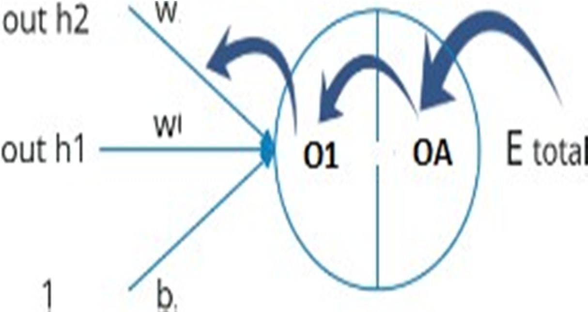
After the above operation, need to start backwards step. To update the weights based onthe error value.

Here, the change in error for the weight w5 will be calculated using the formula Etotal = Etotal outO1 net01. (14) 5 1 01 5

We are spreading in reverse; the first task is to compute the correction for simple errors with respect to the yields O1 and O2. A new weight is determined using

\s