IV. RESULTS

1. Pearson’s Correlation Test

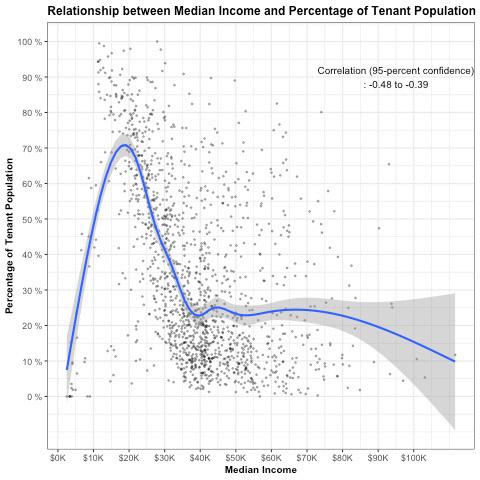
According to the result of Pearson’s correlation test (Table2, Figure1), the median income had a negative relationship and the percentage of foreign-born population had a positive relationship with the percentage of tenant population. The relationships were relatively moderate considering 95-percent confidene interval for correlation were around (+/-) 0.5. Both relationships were statistically significant with sufficiently low p-values.

<Table2. The Result of Pearson’s Correlation Test>

Variable

Median Income 95-percent confidence interval for correlation with the percentage of tenant population

-0.48 to -0.4

Percentage of Foreign-born Population 0.58 to 0.64

Bold text indicates significance at 95-percent confidence level

<Figure1. Scatterplot of the result of Pearson’s Correlation Test>

IV. ResULts

2. ANOVA/Tukey HSD

According to the result of the ANOVA/Tukey HSD test (Table3, Figure2), the tracts with a majority Hispanic-Latino population or black/African American population had a higher percentage of tenant population than white-majority tracts with statistical significance. For transportation mode, the tracts where the public transportation shares the highest mode share tended to have a higher percentage of tenant population than the tracts where driving shares the highest mode share with statistical significance. However, other relationships between the categories under both variables were not statistically significant.

<Table3. The Result of ANOVA/Tukey HSD Test>

Variable

Majority Race

White- Latino White - Asian White - Black White- Other 95-percent confidence interval for correlation with the percentage of tenant population

-0.49 to -0.37 -0.47 to -0.14 -0.36 to -0.21 -1.03 to 0.13

Transportation with the highest Mode Share

No Majority-Car Public Transportation-Car Walking-Car -0.53 to 0.17

0.3 to 0.45

0.06 to 0.23

Bold text indicates significance at 95-percent confidence level

IV. ResULts

<Figure2. Boxplots of the results of ANOVA/Tukey HSD Test>

The tracts where the public transportation share the highest mode share tend to have a higher percentage of tenant population than the tracts where driving shares the highest mode share with statistical significance.

The tracts with majority Hispanic-latino population or black/African American population have higher percentage of tenant population than white-majority tracts with statistical significance.

IV. ResULts

3. Linear Regression

Based on the result of the relationship test, I have built four models. Model1, the initial model, sets the percentage of the tenant population as a dependent variable and median income, race/ethnicity, nativity and mode of transportation as independent variables.

Percentage of Tenant Population

= a*Median Income (10K) + b*Majority Race + c*Transport with the highest Mode Share + d*Percentage of Foreign-born Population + e

For model2, I log-transformed the median income. For model3, I additionally mutated the variable, “percentage of foreign-born population” to the categorical variable by whether foreign-born population is the majority (>50%) or not. Lastly, for model4, I added the interaction term between the median income and transportation mode to the initial model (Table4&Figure4, p.14).

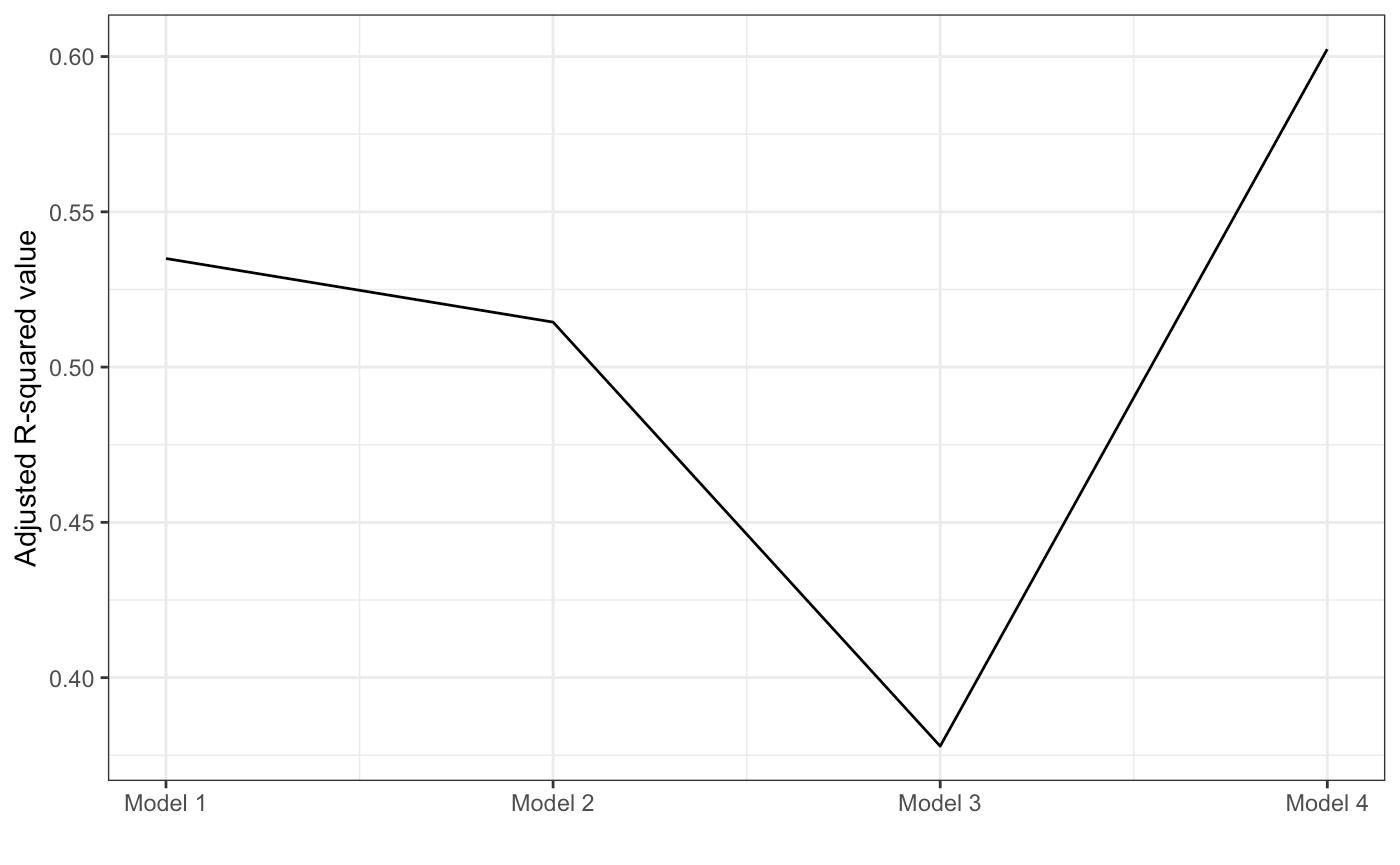
Shown in the graph comparing the adjusted R-squared values of four models (Figure3, p.13), as the R-squared value is the highest in the model4, I selected model4 as the best-fit model. With the R-squared value of 0.61, these independent variables explain 61% of the variation in the percentage of tenants in this dataset.

Median income turns out to have a statistically significant and negative relationship with percentage of tenant population. As the median income increases by $10,000, the percentage of tenant population decreases by 0.06%p, when controlling other variables.

IV. ResULts

age of 0.38%p lower in the tracts where walking accounts for the highest mode share than car-dominant tracts. Also, the percentage of tenant population is an average of 0.55%p lower in the tracts where no single transportation mode takes the highest mode share than car-dominant tracts. These differences are all significant at a 95% confidence level. The other relationships between different categories and percentage of tenant population were not statistically significant.

This is a notable difference when compared to the result of Tukey HSD test which showed the statistically significant and positive relationship between public transportation and the percentage of tenant population, while other relationships were not even statistically significant. This implies there’s more complex relationship between the tenure and mode of transportation, presumably influenced by other factors including median income or race/ethnicity.

I further delved into the potential interaction between median income and mode of transportation with the interaction term. The positive and statistically significant coefficient for the interaction between median income and transportation mode (except the “No Majority” with statistically insignificant p-value) tells us that median income has more of an effect on the percentage of tenant population for the tracts where public transportation and walking is the major transportation than it does for ones with cars.

More specifically, the interaction plot (Figure5) shows that given the condition that sample tracts’ median income is zero, the tracts where the majority of people drive tend to have higher percentage of tenant population than the tracts with public transportation or walking. However, as the median income of tracts increases, the trend begins to reverse at some point that tracts where alternative

IV. ResULts

mode is mainly used have higher percentage of tenant population than majority-driving tracts.

For race/ethnicity, with “white” population as the base case, the percentage of tenant population is an average of 0.17%p higher in the tracts where Hispanic-Latino population accounts for the highest racial proportion. However, the relationships between white and Black/Asian majority tracts were not statistically significant, when controlling other variables.

Lastly, the percentage of foreign-born population had a positive relationship with the percentage of tenant population. For every 1%p increase in the census tract’s percentage of foreign-born population, the value of percentage of tenant population increases by 0.86%p. It is statistically significant at a 95% confidence level.

<Figure3. Comparison of Adjusted R-squared Values>

IV. ResULts

<Table4. Result of Linear Regression>

Model1 Model2 Model3 Model4

Median Income(/10K) -0.04 *** (p = 0.00)

Log(Median Income(10K) -0.12 *** (p = 0.00) -0.13 *** (p = 0.00) -0.06 *** (p = 0.00)

Majority Hispanic-Latino (compared to White)

Majority Asian (compared to White)

Majority Black (compared to White)

Majority Other (compared to White)

No Majority Transport Modal Share (compared to car)

Public Transportation with the highest Modal Share (compared to car)

Majority Walking (compared to car)

Percentage of Foreign-born Population

Majority US-Born

Interaction: No Majority Transport and Median Income 0.19 *** (p = 0.00) 0.19 *** (p = 0.00) 0.32 *** (p = 0.00) 0.17 *** (p = 0.00)

-0.01 (p = 0.81) -0.01 (p = 0.91) 0.24 *** (p = 0.00) -0.01 (p = 0.88)

0.05 * (p = 0.03) 0.07 ** (p = 0.01) 0.21 *** (p = 0.00) 0.03 (p = 0.15)

0.27 (p = 0.11) 0.27 (p = 0.12) 0.35 (p = 0.07) 0.22 (p = 0.16)

-0.31 * (p = 0.01) -0.39 ** (p = 0.00) -0.37 ** (p = 0.01) -0.55 ** (p = 0.00)

0.20 *** (p = 0.00) 0.19 *** (p = 0.00) 0.30 *** (p = 0.00) -0.08 (p = 0.12)

0.09 *** (p = 0.00) 0.04 (p = 0.16) 0.10 *** (p = 0.00) -0.38 *** (p = 0.00)

0.85 *** (p = 0.00) 0.86 *** (p = 0.00) 0.86 *** (p = 0.00)

-0.03 (p = 0.52)

0.15 (p = 0.13)

Interaction: Majority Public Transportation and Median Income 0.07 *** (p = 0.00)

Interaction:

Majority Walking and Median Income 0.13 *** (p = 0.00)

1462 1462 1462 1462

R2

0.54

*** p < 0.001; ** p < 0.01; * p < 0.05.

0.52 0.38 0.61

IV. ResULts

<Figure4. 95-percent Confidence Intervals for Model 4 Coefficients>

<Figure5. Interaction Plot between Median Income and Mode of Transportation>