2)Solar and Orbital Variations

William Herschel theoretical and observational work provided the foundation for modern binary star astronomy; he was the first to recognize the orbital relationship that may physically link together double stars (Poyet, 2017a-b) and not consider them to be just fortuitous alignments «I may therefore immediately go to the second, which treats of binary sidereal systems, or real double stars» (Herschel, 1803). He is also the discoverer in 1800 of infra-red radiations (IR), that characterize the absorption spectrum of trace gas that we have studied in this work, water vapor first, though it is unclear whether this discovery happened while testing solar filters to observe solar spots or rather pioneering the use of astronomical spectrophotometry, using prisms and temperature measuring equipment to record the wavelength distribution of stellar spectra.

But the reason to mention Herschel’s work here, is that he ventured into the speculation that there would exist a link between solar irradiance and climate. This was based on an apparent correlation he had found between sunspot numbers and the price of wheat, and Herschel (1801) reported «The result of this review of the foregoing five periods is, that, from the price of wheat, it seems probable that some temporary scarcity or defect of vegetation has generally taken place, when the sun has been without those appearances which we surmise to be symptoms of a copious emission of light and heat» p. 316. The hypothesis that there would exist such a relationship did not bring him fame, as this had already happened thanks to his discovery of Uranus on March 13, 1781 but rather mockery and elicited guffaws (from Lord Brougham among others). It took some time before this relationship would be further investigated and confirmed by two researchers in Israel who have found a statistical link between the activity of the Sun and the price of wheat in seventeenth-century England, confirming that “at the point in the solar cycle when sunspots were least likely, wheat prices tended to be high” (Pustilnik and Yom Din, 2004).

This is well summed up by Pustilnik and Yom Din (2004) «The results of our study show: a) The coincidence between the statistical properties of the distributions of intervals between wheat price bursts in medieval England (1259-1702) and intervals between minimums of solar cycles (1700-2000); b) The existence of 100% sign correlation between high wheat prices and states of minimal solar activity established on the basis of 10Be data for Greenland ice measurements for the period 1600-1700. These results imply a causal connection between solar activity and wheat prices in medieval England. This conclusion is consistent with our conceptual model of the causal chain, consisting of “solar activity – cosmic ray intensity – terrestrial weather – wheat production – wheat price” that presented in this work ». They add that for all ten solar cycles between 1600 and 1700, high wheat prices coincided with low activity, and vice versa and that «the probability of this happening by chance is less than 1 in 500».

Therefore, changes in solar activity alter the strength of the solar wind, i.e. the stream of charged particles that flows from the Sun throughout the solar system (Parker, 1958173). When the solar wind is strong, it is more difficult for charged particles from deep space to penetrate Earth's atmosphere. Once in the atmosphere, these cosmic rays collide with molecules in the air to produce ions, which help cloud droplets to form. So in periods of high solar activity the skies are less cloudy. Over the past few years, satellite observations have confirmed this link as well as results from the Earthshine project which studies the modulation of the albedo (Pallé et al., 2004a). One should remember that a change of albedo of a tiny 3% (say from 31% down to 30%) is equivalent to the warming anticipated by a doubling of [CO2]. The tidal forcing of the planets on the solar surface and solar wind has been explored by Poulos (2016; 2020).

In fact this line of reasoning has been explored probably first by Denton and Karlén (1973) using C14 variations measured from tree rings “Short-term atmospheric C14 variations measured from tree rings correlate closely with Holocene glacier and tree-line fluctuations during the last 7000 yr. Such a correspondence, firstly, suggests that the record of short-term C14 variations may be an empirical indicator of paleoclimates and, secondly, points to a possible cause of Holocene climatic variations. The most prominent explanation of short-term C14 variations involves modulation of the galactic cosmic-ray flux by varying solar corpuscular activity”, then Tinsley and Deen (1991) and later by Svensmark and FriisChristensen (1997) and Marsh and Svensmark (2000), Carslaw et al. (2002), Kirkby (2007) as reminded by Veizer (2005) “In this alternative, an increase in TSI results not only in an enhanced thermal energy flux, but also in more intense solar

173When Eugene Parker submitted a paper on his discovery of solar wind in 1957, two eminent reviewers rejected the paper.

However, since Chandrasekhar was editor of the Astrophysical Journal and could not find any mathematical flaws in Parker's work, he went ahead and published the paper in 1958.

wind that attenuates the CRF174 reaching the Earth. This, the so-called heliomagnetic modulation effect reflects the fact that the solar magnetic field is proportional to TSI and it is this magnetic field that acts as a shield against cosmic rays. The terrestrial magnetic field acts as a complementary shield, and its impact on CRF is referred to as geomagnetic modulation” (Beer et al., 2002). As Carslaw et al. (2020) sum it up “It has been proposed that Earth’s climate could be affected by changes in cloudiness caused by variations in the intensity of galactic cosmic rays in the atmosphere. This proposal stems from an observed correlation between cosmic ray intensity and Earth’s average cloud cover … the observation has raised the intriguing possibility that a cosmic ray–cloud interaction may help explain how a relatively small change in solar output can produce much larger changes in Earth’s climate”.

To summarize, what could be classified under “astronomical influences” on the climate may be decomposed under:

• either direct solar influences (Le Mouël et al., 2008), e.g. variations in TSI due to changes in solar activity (Hoyt and Schatten, 1993, 1997; Shapiro et al., 2011; Soon et al., 2015) which could be as high as ± 4.5 W/m2 since 1750 (Judge et al., 2020) as compared to IPCC estimate for 2XCO2 anthropogenic forcing of 2.2 ± 1.1 W/m2 or of just 1.3 W/m2 for Smirnov (2020), or indirectly through modifications of the cloud formation processes due to changes in the CFR received, or through other amplification mechanisms (Shaviv, 2008; Rabeh et al., 2011); • or indirectly through orbital variations (Javier, 2016a), i.e. eccentricity (as the Earth is subject to the influence of the other planets, especially the closest giants Jupiter and Saturn, the Earth’s orbit eccentricity changes with a major beat of 413,000 years and two minor beats of 95,000 and 125,000 years, the two precession movements (axial of 26,000 years and the slow rotation of the elliptical orbit around the focus of the ellipse closest to the Sun in a period of 113,000 years), obliquity175 (variations of the inclination of the rotation axis over the ecliptic where the axial tilt varies between 22.1° and 24.3° over the course of a cycle that takes 41,000 years, the last maximum having been about 10000 years ago), and finally the small nutation (period of 18.6 years, the same as that of the precession of the Moon's orbital nodes), all which lead to changes of the TSI received by the Earth. Into this latter effect, one could also add longer term variations linked to the travel of the solar system into the inter-stellar environment or even into the galactic space.

Because of the earth’s elliptical orbit the natural variation of incoming solar irradiance at TOA (i.e. 100 km per NASA) fluctuates 90 W/m2 from perihelion (1,413 W/m2) to aphelion (1,323 W/m2) and because of the earth’s tilted axis the total solar insolation on a horizontal surface at the top of the atmosphere and 40 N latitude fluctuates 638 W/m 2 between winter and summer176. One should further notice that eccentricity is the only factor that changes the amount of energy received by the Earth. However, as the Earth’s orbit has currently an eccentricity of 0.016 and is thus quite circular (eccentricity varies from 0.005 to 0.06), the change in insolation between Perihelion (closest to the Sun) and Aphelion (farthest to the Sun) respectively now at January and July, is always small, currently about 6.4%. The other changes entail variations in the distribution of the energy over the various areas, i.e. NH and SH, and respectively continents and oceans (and cloud systems) as they are not evenly distributed in between the two hemispheres. Therefore remains two major sources of astronomical influences on climate change, one that will deal directly with the Sun and its activity and the other that will be referred to in generic terms as Milankovitch theory (Levrard, 2005) even though strictly speaking Milankovitch (1949) asserted that the main determinant of a glacial period termination is high 65° N summer insolation, and a 100 kyr cycle in eccentricity which induces a non-linear response that determines the pacing of interglacials, whereas modern calculation means available today show that a more complex combination of orbital parameters determines a signature which triggers the start or enable the end of a glacial period.

It is noteworthy that even users of climate models (models that we dismiss because they fail to represent observations and are highly parametrized to reflect great and inappropriate sensitivity to CO 2) do conclude that orbital parameters are more important than GHGs, as Vettoretti and Peltier (2011) who use the ocean-atmosphere version of the Community Climate Model to compare the effects of decreasing CO2 concentrations with those of the orbital influence on snow accumulation and the abyssal circulation in the Atlantic. They come to a somewhat challenging conclusion for the Early Anthropogenic Hypothesis postulated by (Ruddiman, 2007), that is, astronomical trigger is a more important driver of ice accumulation than CO2., i.e. “Results from this set of multi-century sensitivity experiments demonstrate the

174CRF, i.e. Cosmic Ray Flux 175Earth changes of obliquity are stabilized by its large satellite , the Moon, whereas Mars for example undergoes wild and chaotic changes of obliquity that would make the existence of life difficult anyway (Touma and Wisdom, 1993; Laskar and Robutel, 1993;

Laskar et al., 2004) 176According to IPCC AR5 the heat added to the atmosphere by the increased CO 2 over the 261 years from 1750 to 2011 is 2 W/m 2 .

IPCC AR5’s worst, worst, worst, worst case modeled scenario is Representative Concentration Pathway (RCP) 8.5 W/m2 .

relative importance of forcings due to insolation and atmospheric greenhouse gases at the millennial scale, and of Atlantic ocean overturning strength (AMOC) at the century scale. We find that while areas of perennial snow cover are sensitive to GHG concentrations, they are much more sensitive to the contemporaneous insolation regime ”, and they further add “Our analyses demonstrate that while cool NH summers are a prerequisite for glacial inception, a low value of obliquity is most important in determining the strength of the inception process, followed in order of importance by the magnitude of the eccentricity-precession forcing, which dictates the timing and magnitude of the NH summer cooling through geologic time. The minimum and maximum values of carbon dioxide concentrations inferred from ice core records characteristic of the late Pleistocene glacial inception periods also influence the strength of the inception phenomenon, in fact to the same degree as the eccentricity-precession forcing” (Vettoretti and Peltier, 2011).

The incident solar flux on the globe, of power (on an annual average) 173 PetaWatt (173 10 15 W) is ten thousand times the power corresponding to the consumption of primary energy (13,865 Mtoe / year in 2018) by all humanity, see Figure 27, p. 90. The part of the incident solar absorbed by the globe, about two thirds, is compensated, over the year, but fairly exactly, to the nearest thousandth, by the thermal infrared radiation from the globe to the cosmos of the order of 120 PW in January and 125 PW in July. This infrared thermal radiation from the globe to the cosmos, subsequently designated by the Outgoing Long-wave Radiation (OLR), averaged over the globe, varies between 234 W/m² in January and 244 W/m² in June-July while the sunshine, on average over 24 hours, at the top of the air varies between 353 W/m² in January and 331 W/m² in June (Earth at aphelion).

The Sun represents 99% of the mass of the solar system and it is at first hard to imagine how the planets would influence it and create some variability. But one must remember that all stars are sort of self-regulating systems that obey to an hydrostatic equilibrium. Energy is generated in the star's hot core, then carried outward to the cooler surface, this is the outward force of pressure which is balanced by the inward force of gravity (Djorgovski, 2004; Malherbe, 2010). If we consider a small cylindrical element between radius r and radius r + dr in the star of surface area = dS to which is applied the inward pressure P (r+dr) and outward pressure P(r) for a mass = Δm with the mass of gas in the star at smaller radii = m = m(r) then the inward force applying on the small element is the gravity given by: Fg = - (Gm Δm) / r2 then the Pressure (net force due to difference in pressure between upper and lower faces) is: Fp = P(r)dS - P(r + dr)dS = P(r)dS - [ P(r) + (dP/dr) dr] dS = - (dP/dr) dr dS and as Δm = ρ dr dS applying Newton's second law ΣF = m ϒ leads as the star is in static equilibrium and acceleration=0 to: - (Gm Δm) / r2 - (dP/dr) dr dS = 0 substituting for Δm one obtains: - (Gm ρ dr dS) / r2 - (dP/dr) dr dS = 0 and therefore: dP dr =−( G m r 2 ) ρ (158)

stellar structure equation stating hydrostatic equilibrium.

Stating the conservation of mass, let r be the distance from the center and Density as function of radius is ρ(r), let m be the mass interior to r, then conservation of mass implies that: dm = 4πr2 ρ dr which leads to: dm dr =4 π r 2 ρ (159) stellar structure equation stating the conservation of mass.

we can combine these two equations (dP / dm) = (dP / dr) x (dr / dm) = - ( Gm / r2 ) ρ x (1 / 4πr2 ρ ) and thus: dP dm =−( G m 4π r

4 ) (160)

The interior of a star contains a mixture of ions, electrons, and radiation (photons). For most stars the ions and electrons can be treated as an ideal gas and quantum effects can be neglected, thus the total Pressure: ΣP = Pi + Pe + Pr = Pgas + Pr

where Pi is the pressure of the ions, Pe is the electron pressure, Pr is the radiation pressure.

The gas pressure Pgas is given by the equation of state for an ideal gas: Pgas = nkT where n is the number of particles per unit volume; n = ni + ne, where ni and ne are the number densities of ions and electrons and in terms of the mass density: Pgas = ( ρ / μ mH ) kT where where mH is the mass of hydrogen and μ is the average mass of particles in units of mH. Therefore, the ideal gas constant is given by: R = k / mH (R = 8.3 107 erg g-1 K-1) thus:

Pgas =( R μ ) ρ T (161)

The radiation Pressure for a Black Body will be given by: P r a T 4 3 (162)

where a = 7.565 10-16 J m-3 K-4 is the radiation constant. Not going any further into details, one should know that “Gas pressure” is most important in low mass stars while “Radiation pressure” is most important in high mass stars.

The reason why this short presentation was developed is that one needs to understand that a star like the Sun (and all others neither collapsing or exploding while they remain on the main sequence for billions of years) is in a relative equilibrium between inward gravitational forces and outward pressure forces, therefore even though all the planets of the solar system just represent 1% of the mass of the entire system, it is not unconceivable that their motion around the Sun may create some solar variability, by creating small disturbances to the equilibrium of forces the Sun depends on. What would at first look like a form of "astrology" gets physical sense once this notion of disturbance to a precarious equilibrium is better understood. Of course, the planetary beat is not going to lead to a great imbalance in between the internal solar gravitational forces and outward pressure forces but slight changes due to planetary triggers can entail a new equilibrium leading to some form of solar variability.

This possibility of an extreme importance for our subject has been explored by Abreu et al. (2012) and leads to key conclusions “The excellent spectral agreement between the planetary tidal effects acting on the tachocline and the solar magnetic activity is surprising, because until now the tidal coupling has been considered to be negligible. We therefore suggest that a planetary modulation of the solar activity does take place on multidecadal to centennial time scales”. The tachocline, invented by Spiegel and Zahn177 (1992) is the transition region of stars of more than 0.3 solar masses, between the radiative interior and the differentially rotating outer convective zone. This concept resulted of the work performed for years by Zahn on tidal friction in close binary stars (1977) and models of circulation and turbulence in rotating stars (1992) and Zahn also worked on understanding tidal effects produced by solar and extra-solar planets. It should be noted here that the superadiabaticity δ, is a dimensionless measure of the stratification of the specific entropy in a medium, and enables to separate a radiative zone δ < 0 (stable stratification) from a convection zone δ > 0 (unstable stratification). Somewhere at the level of the tachocline, characterized by a very large shear, the bottom of the convection zone δ changes sign. δ becomes negative and very small in what is referred to as the “overshoot layer”, where it is believed that strong toroidal flux tubes ( 10 ∼ 5 G178) are stored prior to the eruption of the sunspots179 .

How a tiny modification (1 part in 104 or 105) of the entropy stratification is produced by the tidal forces remains unknown. But Abreu et al. (2012) state “we can think of a resonance effect mediated by gravity waves. Since this coupling takes place in the tachocline, the tidally excited gravity waves (Goldreich & Nicholson 1989a,b; Goodman and Dickson 1998; Barker & Ogilvie 2010) may be modified by the shear of the environment ”. But the conclusion of Abreu et al. (2012) is of great relevance “Here we suggest that a full understanding of the long-term solar magnetic activity can only be achieved by considering the influence of the planets on the Sun and allowing for internal amplification mechanisms. As a first step in this process we have proposed a simple model describing planetary torques acting on a non-spherical solar tachocline”. Now it must be stated that the solar modulation potential φ180, which can be derived from either the 10Be (polar ice-cores) or the 14C (tree-rings) production rates181, best represents the role of the solar magnetic field in deflecting cosmic rays and observing Fig. 1 and Fig. 5 of Abreu et al. (2012) is very telling for two reasons: 1. the solar modulation potential φ as never been higher than now for the last 9,000 years, thus confirming the exceptional level of solar activity as displayed in Figure 55, p. 150; 2. the comparison between solar activity and planetary torque in the frequency domain shows well known peaks such as the 88 yr Gleissberg and the 208 yr de Vries cycles, but also periodicities around 104yr, 150yr, and

177https://fr.wikipedia.org/wiki/Jean-Paul_Zahn supported Paul Couteau at the Nice Observatory for whom I worked and where I was lucky to participate in visual double stars measurements, see Poyet (2017a; 2017b). 178https://en.wikipedia.org/wiki/Gauss_(unit) 179Sunspots are the surface manifestation of a strong internal toroidal magnetic field leading to the observed spectral Zeeman effect; see Hale (1908) and Hale et al. (1919). 180φ varies in- (anti-) phase with the sunspot number during strong (weak) cycles, in agreement with φ estimates from ice core records of 10Be concentration, which are in-phase during most of the last 300 years, but anti-phase during the Maunder

Minimum (Owens et al., 2012), see Czechowski et al. (2010) for the definition of the Heliospheric Current Sheet (HCS) tilt angle. 181One should note that 14C and 10Be are both produced by cosmic rays in the atmosphere, but have completely different geochemical properties, because whereas 14C enters the carbon cycle by forming CO2, 10Be becomes attached to aerosols and is removed from the atmosphere mainly by wet deposition.

506yr. Of major importance to our subject is the extraordinarily well visible 506yr frequency displayed by the Fourier spectrum of the annually averaged torque modulus Fig. 5b of Abreu et al. (2012). Thus, the strongest periodicity displayed by the Fourier spectrum of the annually averaged torque modulus, i.e. 506 yr ±6.0, is the average period separating the Roman optimum from the misery of the collapse of the Roman empire, and from thereof from the next medieval optimum, and from this optimum to the next misery of the LIA, and from then to the current modern optimum. Abreu et al. (2012) conclude “Here we suggest that a full understanding of the long-term solar magnetic activity can only be achieved by considering the influence of the planets on the Sun and allowing for internal amplification mechanisms. As a first step in this process we have proposed a simple model describing planetary torques acting on a non-spherical solar tachocline”. The statistical significance of the results obtained is also addressed in Appendix A and Abreu et al. (2012) state “We observe that five of the strongest spectral lines in all three records agree very well. Finally, we determine the probability that these five lines agree by chance using a Monte Carlo technique. We conclude that the chance of a random coincidence is about 5 × 10−7”.

Along the same line of reasoning, this is what led Mörner et al. (2013) in “Pattern in solar variability, their planetary origin and terrestrial Impact” to address the question of the possible planetary modulation of solar variability, “The Sun’s activity constantly varies in characteristic cyclic patterns. With new material and new analyses, we reinforce the old proposal that the driving forces are to be found in the planetary beat on the Sun and the Sun’s motions around the center of mass...” the authors of the special issue “conclude that the driving factor of solar variability must emerge from gravitational and inertial effects on the Sun from the planets and their satellites”.

Therefore, throughout the Holocene it has been possible to identify numerous solar activity cycles which are preserved within various records and known in the literature as the cycles of: • Bray-Hallstatt182 (2,310 yr ±300) displayed on top of Figure 35, discovered by Bray (1968) and confirmed since many times, e.g. (Hood and Jirikowic, 1990; Damon and Sonett, 1991; van Geel, 1998; Vasiliev and Dergachev, 2002; Charvátová and Hejda, 2014; Javier, 2017g; May and Javier, 2017), see Figure 56 ; • Eddy (976 yr ±53) (Eddy, 1976; Javier, 2017g, Lüdecke and Weiss, 2017), the list of Solar Grand Minimum (SGM) potentially related with the Eddy cycle lows, according to Usoskin (2017) and using his dates (adding E for Eddy and B for Bray) is : Maunder (B1-E1-270 BP), Roman (E2-1,260 BP), Greek (E3-2,310 BP), No name (E43,335 BP), No name (E5-4,400 BP), Sumerian (B3/E6-5,275 BP), No name (E7-6170 BP), No name (E7-6,265 BP), Jericho (E8-7,145 BP), Jericho (E8-7,250 BP), Sahelian (E9-8,335 BP), Boreal 2 (E10-9,255 BP), Boreal 1 (B5/E119,465 BP), Preboreal (E12-11,115 BP); • Abreu (506 yr ±6.0), the most prominent of all in the study by Abreu et al. (2012) and the most relevant to the periodicities that correspond to the last known and documented climatic optima, i.e. the Roman, Medieval and Modern; • Suess-de Vries183 (208 yr ±2.4), e.g. (Damon and Sonett, 1991; Stuiver et al., 1995; Yousef, 2000; Bond et al., 2001; Wagner et al., 2001; Rombaut, 2010; Liu, Y, et al., 2011; Lüdecke et al., 2015; Javier, 2017g); • Jose (155-185 yr) “The motion of the sun about the center of mass of the solar system has periodicity of 178.7 yr. The sunspot cycle is found to have the same period” (Jose, 1965; Charvátová and Hejda, 2014); • Gleissberg (88 yr ±13), e.g. (Damon and Sonett, 1991; McCracken et al., 2001; Peristykh and Damon, 2003; Feynman and Ruzmaikin, 2011, 2014), reported by Stuiver and Braziunas (1993) as “The 210 and 88 yr 14C periodicities relate rather unequivocally to solar forcing (...) The 88 yr 14C periodicity has only a minor 18O companion” dismissed by Javier (2017g), but reported as very prominent by Knudsen et al. (2011) between 4,000 and 6,250 years BP and later became remarkably vague from ~3,500 years BP onwards; • the 55-65 yr cluster (Javier, 2017g) or ~60 yr oceanic oscillation (Jevrejeva et al., 2008; Scafetta, 2010) or evidenced by Klyashtorin and Lyubushin (2003) using spectral analysis over 1,000 years, which could be explained by the ~60-year oscillation in the barycentric movement of the Sun due to its ~60-year tri-synodic period produced by the Jupiter–Saturn system184 (Mazzarella and Scafetta, 2011; Gervais, 2016a);

182Named after a cool and wet period in Europe when glaciers advanced, the Hallstatt culture was the predominant Western and

Central European culture of Late Bronze Age (Hallstatt A, Hallstatt B) from the 12th to 8th centuries BC and Early Iron Age Europe (Hallstatt C, Hallstatt D) from the 8th to 6th centuries BC 183Named after Hans Eduard Suess and Hessel De Vries respectively 184A full cycle of Jupiter and Saturn around the sun (J/S Tri-Synodic Cycle) takes 59.6 years, therefore every ~60-years the Earth,

Jupiter and Saturn reach the same relative alignment around the Sun. One can easily dismiss these harmonics, but before doing so, one shall remember first that, for example, the Moon is synchronized with the Earth and it always presents us the same face for very good reasons, and there exists many other resonances, e.g. Mercury is locked to its own orbit around the Sun in a 3:2 resonance. It happens that more 60 satellites do the same with respect to their planets in the solar system and tidal locking is a very well known phenomenon https://en.wikipedia.org/wiki/Tidal_locking

• and the 11 years Schwabe / Wolf cycle of course (Brehm et al., 2021), which is known to have among others effects, a direct impact on Arctic weather as reported by Roy (2018a) “when the winter solar sunspot number (SSN) falls below 1.35 standard deviations (or mean value), the Arctic warming extends from the lower troposphere to high up in the upper stratosphere and vice versa when SSN is above”. This 11 years Schwabe cycle also has a very strong influence on NAO and North Atlantic as shown by Roy (2020) since 1977.

The 11 year cycle was discovered by Christian Horrebow in 1775, later formalized as a periodic variation in 1843 by Samuel Heinrich Schwabe and later organized and numbered by Rudolf Wolf, going back to 1745. This cycle has been known for the longest and thereafter has of course been the most studied and demonstrates at least two important things: 1) how the various components of the terrestrial atmosphere are tightly coupled and interact together and 2) how the cycle originates far from the Sun in tidal forces exerted by several planets on our star. This is remarkable as it shows the complexity of the Earth-Solar-Planetary system which cannot be reduced to a trace gas. Labitzke and Van Loon (1991) report “We describe a 10-12-year oscillation (TTO) in the upper troposphere and lower stratosphere of the Northern Hemisphere in summer... The TTO is in phase with the 11-year solar cycle...The analyses show that the large amplitude of the TTO in the geopotential heights of the lower stratosphere is associated with temperature variations of the same time scale in the upper troposphere”, showing the influence of the 11-year solar cycle on the stratosphere and demonstrating how it impact the troposphere. Stefani et al. (2019) present the 11-year cycle as the result of planetary tidal forces “We discuss a solar dynamo model of Tayler-Spruit type whose Ω-effect is conventionally produced by a solar-like differential rotation but whose α-effect is assumed to be periodically modulated by planetary tidal forcing. Specifically, we focus on the 11.07 years alignment periodicity of the tidally dominant planets Venus, Earth, and Jupiter, whose persistent synchronization with the solar dynamo is briefly touched upon”. Other evidences are provided, such as (Zhai, 2016) or Misios et al. (2018) “Influences of the 11-y solar cycle (SC) on climate have been speculated, but here we provide robust evidence that the SC affects decadal variability in the tropical Pacific. By analyzing independent observations, we demonstrate a slowdown of the Pacific Walker Circulation (PWC) at SC maximum”. This is a perfect illustration, at the shortest and most reproducible frequency possible, i.e. 11 years, of the planetary influence on solar activity and of its further action on our atmosphere and climate.

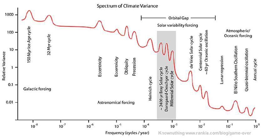
Figure 54. A periodogram185 shows how periodicities (either of orbital or solar origin) dominate climate change at all temporal scales. The 150 Myr Ice Age cycle has produced four Ice Ages in the last 450 million years. It is proposed to be caused by the crossing of the galactic arms by the Solar system (Veizer, 2005). The 32 Myr cycle has produced two cycles during the Cenozoic era, the first ending in the glaciation of Antarctica and the second in the current Quaternary Ice Age. It is proposed to be caused by the vertical displacement of the Solar system with respect to the galactic plane 186. The orbital cycles are well visible (eccentricity, obliquity, precession). The millennial climate cycles (grey band) regroup most of the known solar cycles aforementioned. Short term climate variability is dominated by the El Niño-Southern Oscillation. Adapted by Javier (2017c) from Maslin et al. (2001).

185In signal processing, a periodogram is an estimate of the spectral density of a signal. The term was coined by Arthur Schuster in 1898 186Rampino and Caldeirac (2020) have detected a 32-million year cycle in sea-level fluctuations over the last 545 Myr. They consider various tectonic mechanisms to explain the sea level variations, including a variation of the ocean-floor spreading rates but do not dismiss the astronomical origin to which this 32 Myrs cycle has been attributed here.

Because chronological uncertainties of paleoclimate time series are of an order of magnitude of 1%-2% of the absolute age, for example, between 100 and 200 years for a 10,000 year old sample, this typically leads to make it difficult to try to identify short cycles (e.g. Gleissberg, de Vries) beyond the Holocene. Furthermore, as a general rule, the longer the cycle, the more significant the impact is on the climate (see Figure 54), e.g. the Bray-Hallstatt 2475 yr cycle is very well visible on top of Figure 35 and more significant than shorter cycles. Some high-energy cosmic rays entering Earth's atmosphere collide hard enough with molecular atmospheric constituents that they occasionally cause nuclear spallation reactions. Fission products include radionuclides such as 14C and 10Be that later settle on the Earth's surface.

Therefore, 14C and 10Be cosmogenic isotope records are considered direct proxies for solar activity, and are extracted from trees, sediments, ice cores (e.g.: McCracken et al., 2001; Muscheler et al., 2020; Neff et al., 2001; Ogurtsov et al., 2002; Steinhilber et al., 2012; Vasiliev and Dergachev, 2002), in long sunspot sequences (Ogurtsov et al., 2002), in aurora records (Scafetta and Willson, 2013) and others (e.g. Hoyt and Schatten, 1997). Interestingly, similar solar cycles are also found on a Late Miocene lake system revealed by biotic and abiotic proxies, i.e. by the off-shore sedimentation rates of the Tortonian Vienna Basin which revealed patterns resembling well Holocene solar-cycle-records (Kern et al., 2012) and therefore indicate that they operate not on thousands or tens of thousands of years (e.g. Holocene) but over millions or tens of millions of years (i.e. Cenozoic). These solar cycles are of great relevance as variations of the TSI are considered marginal by IPCC and therefore too small to be responsible of climate change, but in fact as reported by Safetta (2019) “the total solar irradiance forcing is still highly debated because some records show a secular variability as low as 0.6 W/m2 since 1700 to present (Wang et alii, 2005) while others show a very large secular variability up to 6 W/m2 during the same period (Egorova et alii, 2018a); 2) there are several indications that the sun induce climatic changes through a cosmic ray forcing that could directly modulate the cloud system (Kirkby, 2007; Svensmark et alii, 2017). This would be a different kind of solar related forcing that is completely missing in the GCMs”. Of course, depending on whether one uses the values of Wang et al. (2005) or those resulting from the model of Egorova et al. (2018a) the changes of TSI are so important that the Sun passes from a backseat in the climate change distribution role to the forefront.

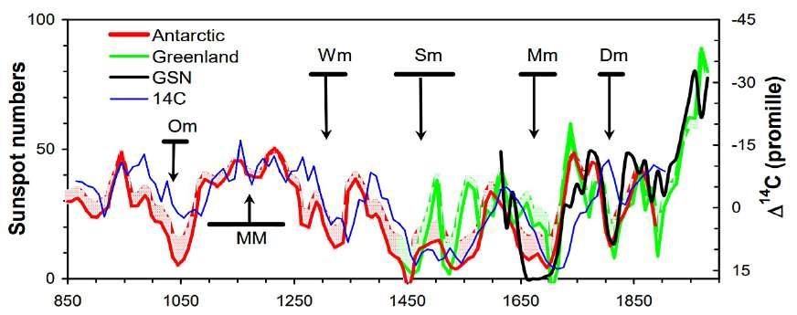
Figure 55. Time series of the sunspot number as reconstructed from 10Be concentrations in ice cores from Antarctica (red) and Greenland (green). The thick black curve shows the observed group sunspot number since 1610 and the thin blue curve gives the (scaled) 14C concentration in tree rings, corrected for the variation of the geomagnetic field. The horizontal bars with attached arrows indicate the times of Great Minima and Maxima: Dalton minimum (Dm), Maunder minimum (Mm), Spörer minimum (Sm), Wolf minimum (Wm), Oort minimum (Om), and Medieval Maximum (MM). From Usoskin et al. (2018).

One should observe at least two things here, first and again we mainly deal with models due to the lack of direct measurements of solar radiation on climatological time scale187, second that depending on how the quiet Sun is reconstructed and other parameters, the TSI can vary a lot, e.g. > 4 W/m2 over the 1600-2000 period (Haigh, 2003), in which case there is an easy and strong case supporting the observations made, which attest the close link between solar variability and climate change, including the precipitations and monsoons, e.g. as mentioned by Neff at al., 2001 “The excellent correlation between the two records (i.e. δ18O et Δ14C) suggests that one of the primary controls on

187TSI measurements have been made from satellites since 1979 but each individual instrument records only last for a number of years and each sensor suffers degradation in orbit. Thus, the construction of a composite series (or best estimate) of TSI from overlapping records from several successive satellites becomes a complex task and many corrections are necessary to compensate for problems of sometimes unexplained drift and uncalibrated degradation in the time-series (Haigh, 2003, 2007).

The Active Cavity Radiometer Irradiance Monitor (ACRIM) TSI composite is such an example, see Scafetta and Willson (2014). For the controversy ACRIM-PMOD see Willson (2014) and Scafetta et al. (2019).

centennial to decadal scale changes in tropical rainfall and monsoon intensity during this time are variations in solar radiation”. But more importantly, the level of solar activity beginning in the 1940s is exceptional, the last period of similar magnitude occurred around 9,000 years ago, i.e. during the warm Boreal period, e.g. (Solanki, et al., 2004; Usoskin, et al., 2007; Usoskin et al., 2018; Wu et al., 2018). This is also confirmed by Lean (2018) who reports “The new estimates suggest that total solar irradiance increased 0.036 ± 0.009% from the Maunder Minimum (1645–1715) to the Medieval Maximum (1100 to 1250), compared with 0.068% from the Maunder Minimum to the Modern Maximum (1950–2009)”, i.e. 1.88 times more for the modern maximum than for the MWP from the maunder minimum used as a reference. This is very well visible on the sunspot reconstruction from Usoskin et al. (2018) reproduced in previous Figure 55.

The Sun was at a similarly high level of magnetic activity for only ~10% of the past 11,400 years. Almost all earlier highactivity periods were shorter than the present episode. Reconstructions of solar activity levels into the distant past (Solanki et al., 2004) indicate that the overall level of solar activity since the middle of the twentieth century stands amongst the highest of the past 10,000 years, e.g. “the modern Grand maximum (which occurred during solar cycles 19–23, i.e., 1950-2009) was a rare or even unique event, in both magnitude and duration, in the past three millennia ” (Usoskin al., 2014). Solar cycles and variations of the Earth's orbital parameters determine the climate and this is well summed up by Scafetta et al. (2017a) “In fact, the magnetic activity of the sun and, probably, also the planetary motions modulate both the solar wind and the flux of the cosmic rays and interstellar dust on the earth with the result of a modulation of the clouds coverage”. This is why the explanation of the transmission of the variations of solar activity to the Earth climate cannot be limited to changes in TSI, even though there is still a lot to argue about the “Solar Constant” (Eddy, 1977), which does seem to only have its name constant!

Astronomers are far more cautious than “climatologists” with respect to the supposed stability of the Solar Constant and therefore the TSI, e.g. Lockwood et al. (1992; 1997) stated “This suggests that the Sun is in an unusually steady phase compared to similar stars, which means that reconstructing the past historical brightness record, for example from sunspot records, may be more risky than has been generally thought”. Two years earlier, Lockwood and Skiff (1990) reported after a large scale survey of the variability of stars comparable to the Sun “ Nearly 200 years of daily sunspot records teach us that the most visible manifestation of solar activity vary unpredictably. Every 11-year cycle is unique. The variation of the total solar output, measured only for slightly less than one ll-year solar cycle,leads us to think that long-term variations are quite small--only 0.1% or so. But to contain this minuscule variation requires the delicate and continual balancing between larger competing effects, the flux deficits associated with sunspots and the flux excesses associated with faculae Stellar photometry offers little assurance that the solar variability actually measured thus far provides an accurate long term prognosis. Indeed, many stars quite similar to the Sun demonstrably vary by amounts much larger than the Sun has over the last decade. Thus we conclude, considering the Sun among the stars, that the present short record of solar variability is remarkable only in its present restraint”.

With regards to other similar stars (spectrum, luminosity, temperature, etc.) the expected TSI variability over longer periods must be far greater than that the IPCC use (0.1%). One can plot the stellar total irradiance measured at 1 astronomical unit versus the color temperature of the stellar photosphere in degrees Kelvin in sort of a HertzsprungRussell Diagram. Most main-sequence stars fall along a curved line going from the upper left corner to the lower right corner. The Sun is a main-sequence star (G0) with a color temperature of 5880 °K and an irradiance of 1367 W/m 2, i.e. the mean value of the so-called Solar Constant (SC). Hoyt and Schatten (1997) remind that “Five billion years ago, the sun began as a late G-class star, perhaps G7 to G9, with an initial irradiance at 1 astronomical unit of about 1000 W/m 2 and a color temperature of approximately 5400 K. Since then it has steadily warmed up, with a 30% increase in luminosity, and its color has changed from reddish to yellow” and is known as the faint Sun paradox188 .

But more importantly, Hoyt and Schatten (1997) are extremely cautious with respect of the supposed stability of the TSI as measured over the short period where we have instrumental records. Hoyt and Schatten (1997) assert “The results of the Hipparchus satellite experiment that detected variations in light output of numerous stars. The main sequence reveals that stars both brighter and dimmer than the sun display more variability than the sun itself. Even though the sun varies, it is one of the more stable stars. The sun's level of activity is about average, but its variations in brightness are well below average. This suggests that in the last two solar cycles, we have only seen a small portion of the brightness variations we would see if we observed many solar cycles” - bold added.

188https://en.wikipedia.org/wiki/Faint_young_Sun_paradox

This is a clear message, that “climatologists” should better listen to, the TSI as measured is not representative of the Sun's longer term variations. In that respect, both Lockwood and Skiff (1990) and Baliunas and Vaughan (1985) found that the variations in the total radiative output from solar-type stars exceeded the currently observed solar-constant variations (from spacecraft over the last decade) by nearly a factor of 4.

It would be preposterous to think that our instrumental records are telling us anything valuable of the long term, not even speaking of geological times but simply of thousands or tens of thousands of years. From thereon, Hoyt and Schatten (1997) make the 3 following assumptions “Excluding remote alternatives, this suggested the following: 1.) The sun may undergo irradiance variations several times larger than any we have seen during the past decade. 2.) Compared with other solar-analog stars our sun is highly unusual because it has especially quiescent radiative output. 3.) Our terrestrial position in the heliosphere (the Earth always lies close to the sun's equator, since the tilt of the sun's rotation axis, BO, relative to the ecliptic plane is a small angle, 7.25°) provides a special vantage point that reduces the observed solar-irradiance variations”.

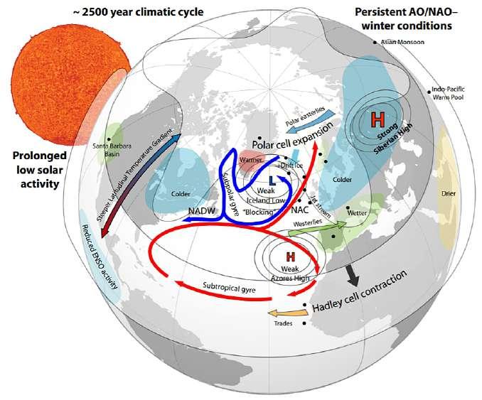
Figure 56. Effect of the ~2500-year Bray(Hallstatt) solar cycle on the climate organization, Source: Javier Vinós public data.

In fact, the three hypothesis have been listed not to be suspected of dishonesty but the third does not appeal to me for a number of reasons, to say the least. As the probability of 2) is very low, indeed, only remains 1) and one must consider that variations of the TSI of up to 4 times what has been measured so far are the most probable alternative. Furthermore, Beer et al. (2002, 2006) mention that even small changes of the TSI are accompanied by far greater changes in the UV part of the solar spectrum (Pagaran et al., 2011; Ermolli et al., 2013), modifying the stratosphere response which is further coupled down to the troposphere (Haigh and Blackburn, 2006). For example, values derived by Lean (2018) show of a factor of 5.66 in between the UV and visible Solar and Spectral Irradiance (SSI) changes respectively.

In a series of papers dealing with the climate during the Holocene, that will certainly prove seminal in the future, Javier (Vinós) addressed many aspects of how the Earth evolved from the time it exited from the LGM and entered the Holocene up to the current modern global warming, and specifically addressed the Bray solar cycle in two articles (Javier, 2017d-e) and one with May and Javier (2017). The last occurrence of the Bray cycle, identified as B2 on Figure 35 and which corresponds to the transition from Sub-Boreal to Sub-Atlantic had already been identified by van Geel et al. (1998) as a major disruption between the Bronze-Age to Iron-Age transition in NW Europe, period during which an abrupt climate change around 850 BC was testified by the sharp rise of the 14C content of the upper atmosphere which was caused by a weakening in solar activity, leading to an increase of the cosmic ray flux and a decrease of the temperature through various mechanisms, including but not limited to a reduction or change of distribution of the

ozone layer (including variation at the tropopause and stratosphere), planetary waves, increased cloudiness and precipitations, among others.

This cooler and wetter climate on middle and high latitudes on both hemispheres came together with a change to a dryer climate in tropical regions due to a weakening of the monsoonal regimes. This resulted of a change of the latitudinal extension of the Hadley Cell circulation and an expansion of the Polar Cells and a change of trajectory of the main depression systems at mid-latitudes in a more equatorward regime. Javier (2017d-e) adds “El Niño is less frequent altering global precipitation patterns. The North Atlantic displays more AO / NAO winter negative conditions shifting the winter European storm track southwards. Weaker westerlies reduce the Sub-Polar Gyre contribution to the North Atlantic current, increasing winter precipitation over Scandinavia and promoting glacier growth. A stronger Siberian High activates polar circulation and southward drift-ice, cooling northern Eurasia. Greenland undergoes a temperature inversion. Black dots represent proxy locations displaying a prominent 2500-year periodicity” and all these effects are well represented and summarized on Figure 56. In fact, around 2,760 ±35 yr BP and 2,620 ±20 yr BP, over a very short period of time of sort of 60 years, houses that were built on artificial mounds could not be used any longer and the area could not be farmed and inhabited as the fresh water table rose everywhere in the northern Netherlands and correspond to an increase of Δ14C. van Geel et al. (1998) remind that "The isotope 14C is produced in the upper atmosphere under the influence of cosmic rays... The most energetic cosmic rays are of galactic origin. The fluctuations of in the cosmic ray flux on Earth are mainly caused by changes in the solar wind, which is a low density gas ejected from the Sun, which strongly influences the magnetic field strength around the Earth”. van Geel et al. (1998) have no doubt that the climate change they report came from solar irradiance variations and it seems that apart from “climatologists” all other scientists studying the climate over longer periods have no doubts about the role of the Sun as a major player in the Earth climate regulation.

At that point in the development of our thoughts it is now possible to start putting forward what represents the essence of out understanding, what will be referred to as from now on as the Energetic Balance of Climate. Climate is the response or the Earth system, in physical terms, to energetic stimulations. These stimulations have several origins: the solar flux whatever form it takes, the orbital configuration which determines how much of the former is received by the Earth, the Earth's own energy which is released through geological manifestations (e.g. mainly volcanism but also some other geothermal sources), plus external, occasional and very unwelcome energy supply like the impact with another celestial body (e.g. asteroid, comet, else) and finally the tiny fraction of the energy stored over geological time (e.g. fossil fuels) that is released by anthropogenic processes. The response of the Earth climate system is proportionate to the energy stimulation received and given the fact that all the power consumption by humankind is less than one ten thousandth of the solar energy received, it gives the size of the maximum possible anthropogenic disruption that mankind is able to produce on the Earth system.

Because the response of the Earth climate system is commensurate to the stimulus, one can easily sense that whatever fake arguments used, the anthropogenic perturbation is minuscule compared to the energies at plays. The physical mechanisms invoked to justify the AGW theory are totally unable to generate the level of disruption claimed by its proponents and therefore they keep resorting to strange notions to the physicists, like “forcing” (Myhre et al., 2013) to justify that if CO2 in its own is unable to generate any significant change to the energy budget, which they know, it will still manage to do so by contorted arguments such as “positive or negative feedbacks” etc. This simply does not make sense and the very illustration of the fact that their theory is completely flawed is that their computer models which implement their physical rantings are completely unable to reproduce accurately even the last 200 years, say since LIA. Warming started long before that the anthropogenic emissions have any significance and warming has been very irregularly distributed over the corresponding period. For instance, the globe warmed in an equal way during the 19221941 and 1980-1999 periods whereas models based on [CO2] to explain the temperature profile accelerate the warming a lot for the second period versus the first to reflect the increase [CO 2] content. And they keep doing so for the period 2000-2016 when there has been nearly no warming at all. (this is the “pause”). So on the one hand there is the reality with warming very unevenly distributed over the reference period and on the other hand there are computerized fantasies which keep forecasting an ever accelerating warming to reflect their dogma into the naive relationship equating more [CO2] with an increase in temperature.

One thing is for sure, not only the level of solar activity is unusually high but it has also lasted unusually long as stated by Solanki et al. (2004) “According to our reconstruction, the level of solar activity during the past 70 years is exceptional, and the previous period of equally high activity occurred more than 8,000 years ago. We find that during the past 11,400 years the Sun spent only of the order of 10% of the time at a similarly high level of magnetic activity and almost all of the earlier high-activity periods were shorter than the present episode”, though to be honest the same

authors dismiss the Sun as the sole explanation “the Sun cannot have contributed more than 30% to the steep temperature increase [since 1970]” (Solanki and Krivova, 2003) though they admit serious simplifying assumptions such as "the connection between the relevant solar and terrestrial quantities is linear", among others. The reason why Solanki and Krivova (2003) are in trouble trying to explain the solar influence on climate is probably because they focus to much on TSI and on the sole troposphere response.

As soon as one checks the correspondence between cloud cover and solar cycles, not saying anything about how one may correlate to the other, but just checking the relationship, the result is statistically significant and positive as reported by Udelhofen and Cess (2001) “Results of spectral analyses reveal a statistically significant cloud cover signal at the period of 11 years; the coherence between cloud cover and solar variability proxy is 0.7 and statistically significant with 95% confidence” who also notice that the cloud cover variations are not in phase with changes of the Galactic Cosmic Rays (GCR). At that point, one must admit that solar influence drives the cloud formation mechanisms at the 11 years cycle level, though the mechanisms by which this is achieved is unknown. Udelhofen and Cess (2001) mention that “cloud variabilities may be affected by a modulation of the atmospheric circulation resulting from variations of the solar-UV-ozone-induced heating of the atmosphere”. The reference to this “solar-UV-ozone-induced” heating is odd as it is asserted as if it were a well known mechanism but apart from their paper no other reference is found to the concept. In fact, one must move up into the atmosphere, to the stratosphere to start gathering some clues as to which mechanisms may be at play and in that respect the paper from Marchand et al. (2012) is telling as they assert “Variations in both ozone and temperature in the stratosphere have been linked successfully to solar cycles using observations and model simulations (Gray et al., 2010)” and confirmed by the reference to Gray et al. (2010) “Perhaps the first place to look for solar impact on the Earth’s climate is in the upper atmosphere because it inter-acts most directly with the radiation, particles, and magnetic fields emitted by the Sun. Solar signals in the stratosphere are relatively large and well documented during the past few11 year SCs since satellite observations became widespread” where SC stands for Solar Cycles.

Therefore, assessing the solar influence on the climate, which is obvious at all timescales considered, is made difficult by the need to not only address changes in the TSI and the way physical phenomenons at the particular scale take place (e.g. atmospheric response to the interaction with GCR, charged particle effects, etc.) but also to need address how the different levels of the atmosphere interact with the solar input and how they convey these signals from one level to the next, e.g. the change in stratospheric temperatures and winds due to changes in UV irradiance and ozone production (e.g. and associated planetary waves), have an influence on the underlying troposphere and the surface climate involves stratosphere‐troposphere-ocean coupling chemistry-processes which are far beyond the capabilities of the best GCM software simulation systems available. Is there a need for an strong anthropogenic influence to account for the temperature increase in the models (and off we go, we're done) or is there a need to better understand the extraordinary complexity of the Earth system and accept that the “models” so far need to better account for the natural variability of the climate response to the various triggers it is subject to, I let the reader decide.

While governments and the UN have funneled billions of dollars to computer modelers to create various CO 2 – driven (and other GHGs) climate simulators since the 1970s, far too little attention has been given to the effect of our Sun on Earth climate. From what was seen, the frequency and intensity of sunspot activity has proven profound influence on Earth weather expressing the influence of solar activity on the climate system. It is also notable that the UN/IPCC dismisses quite completely such solar influence as not significant. That is a huge mistake by all serious evidence. IPCC only acknowledge reluctantly that : «However, there is evidence for a detectable volcanic influence on climate. The available evidence also suggests a solar influence in proxy records of the last few hundred years and also in the instrumental record of the early 20th century» (IPCC, 2018a) TAR-12 p. 697. Could they do less ?

The Earth's magnetic field, also known as the geomagnetic field, is the magnetic field that extends from the Earth's interior out into space, i.e. a dipole with magnetic field lines, and interacts with the solar wind, a stream of charged particles emanating from the Sun. The Sun does not only radiate in the visible part of the spectrum and beyond (where the energy varies much more, e.g. UV) but also produces a flux of charged particles, i.e. the solar wind, released from the upper atmosphere of the Sun, called the corona. This plasma mostly consists of electrons, protons and alpha particles with kinetic energy between 0.5 and 10 keV. Therefore, the Sun’s light is only a part of the global energy emitted, the other parts correspond to solar particles and fields which interact in a more subtle way with the Terrestrial Environment (TE), i.e. the Earth, its atmosphere (and certainly not only the troposphere) but also the Earth's magnetosphere.

This is the sum of all these forms of energy originating from the Sun and interacting with the TE, that have made the climate on Earth for hundred of millions of year, plus exceptional contributions from massive volcanic manifestations or from the collision with another celestial body (the bigger the less frequent), often acting as disruptions of various scales, some being so brutal (impactor > 10km) that they lead to a reset of all forms of life on Earth that can take tens of millions of years and redistributes species and habitats. Therefore, even though the variations of the TSI and of the solar constant should be an on-going debate and certainly not considered as settled (there are no long-term instrumental records of the TSI), one should not circumvent the investigation of the mechanisms by which the Sun drives the climate on Earth to the TSI / Troposphere relationship (Maliniemi, 2016; Asikainen et al., 2017; Maliniemi et al., 2019). One can easily sense that very complex interactions take place between all the component displayed on next Figure 57, and that even some stratospheric chemical changes have their origins in the solar–terrestrial coupling. All these phenomenons will have a direct impact on a number of natural oscillations that we will address in a further section - i.e. Natural Oscillations: QBO, ENSO (El Niño - La Niña), AMO, NAO, PDO.

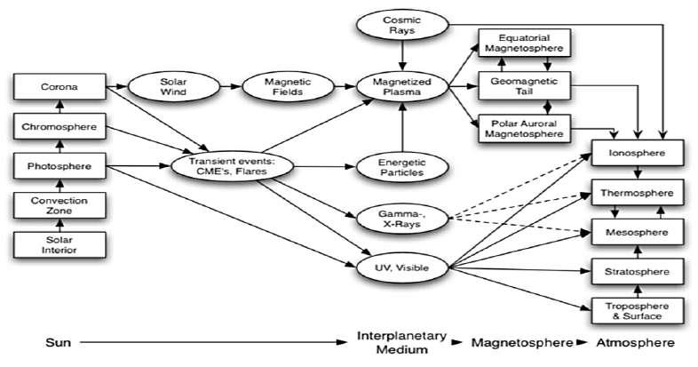
Figure 57. The flow of mass, momentum, and energy from the Sun’s interior through the interplanetary space into the Terrestrial Environment (TE) after (Baker, 2000). Some of the effects of this flow within the coupled system reveal the effect of solar variability on the atmosphere (i.e. Down from the Ionosphere to the Surface), Both normal solar wind flows and transient events are indicated. Source: Javier (2018a).

Solar disturbances are observed to have significant effects in near-Earth space and of among the most remarkable are the high-speed solar wind streams and fast Coronal Mass Ejections (CMEs) often generating strong interplanetary shock waves and are in the geologic records identified and known as Forbush Decreases (FD), i.e. a rapid decrease in the observed galactic cosmic ray intensity following a CME. It occurs due to the magnetic field of the plasma solar wind sweeping some of the galactic cosmic rays away from Earth (Dragić et al., 2011). Svensmark (2019) reminds that it has been for some time (Harrison and Stephenson, 2006; Laken et al., 2010) and demonstrated experimentally “that cosmic rays help the initial formation (‘nucleation’) of small aerosols (1–2 nm), and it was found that by increasing the ionization, the number density of nucleated aerosols increased as well. These results were later confirmed by the CLOUD collaboration experiment at CERN in Geneva” and also state that FD are ideal to test the link between cosmic rays and clouds. In fact, this is what Dragić et al. (2011) did by using the Diurnal Temperature Range (DTR) as an indicator of cloud cover (logically negatively correlated with cloudiness) and demonstrated that the effect of FD on DTR is statistically significant for high amplitude FDs and led to an estimated effect on DTR to be of the order of (0.38±0.06)°C.

These results suggest that this particular chain of related events, from solar activity to cosmic rays, to aerosols (CCN), to clouds is active in the Earth’s atmosphere and plays a role in modulating the cloud cover and therefore the very important albedo, Laken et al. (2010) providing a compelling evidence of a GCR-climate relationship. Other telltales are provided by the cloud-retrievals from the ISCCP satellite program189 which show a strong correlation between low liquid water clouds with galactic cosmic rays from July 1983 to September 1994 and furthermore Gray et al. (2005) state that “Cosmic rays and Total Solar Irradiance variations are often closely correlated”. One should notice that this is just one chain of actions but that as displayed on Figure 57, many others exist and also have an effect on the complex interaction at play between the Sun and the TE and thus on the climate and make it therefore spurious to focus only on

189International Satellite Cloud Climatology Project (ISCCP), https://isccp.giss.nasa.gov/

the TSI / Troposphere radiative balance (not knowing what the TSI has been over long paleoclimatic record) to conclude that the obvious and essential role played by the Sun on the climate cannot be at the origin of climate change, which is just to the contrary of common sense and of all observations.

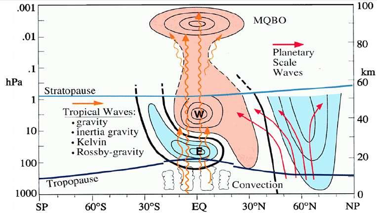
Figure 58. Dynamical overview of the QBO during northern winter. The propagation of various tropical waves is depicted by orange arrows (in the middle), with the QBO driven by upward propagating gravity, inertia-gravity, Kelvin, and Rossby-gravity waves. The propagation of planetary-scale waves (red arrows) is shown at middle to high latitudes. Black contours indicate the difference in zonal-mean zonal winds between easterly and westerly phases of the QBO, where the QBO phase is defined by the 40- hPa equatorial wind. Easterly anomalies are light blue, and westerly anomalies are pink. The Mesospheric QBO (MQBO) is shown above ~80 km. Source: Baldwin et al. (2001).

Svensmark (2019) says that “Temperature variations of the order of 1.0–1.5 K between periods of high and low solar activity, as seen repeatedly over the Holocene period, seem much more likely than the limited changes suggested in those studies [e.g. MBH98, MB99 or Marcott et al., 2013]”. Finally, as pointed out to me by Alain Robichaud (personal communication), “celestial driver of cosmic rays producing cloud condensation nuclei might seem attractive but there are much better explanation for missing source of CCN and ice nuclei in the troposphere”. The atmosphere is part of the biosphere as stated by J. Lovelock190 (Ball, 2014), and ignoring the biological contribution is ignoring the complex relationship that the biosphere maintains with the rest of the Earth's system. Biological particles neglected by physicists might explain a significant part of uncertainties related to clouds in climate models.

Robichaud (2018) adds “Bacteria (the best ice nuclei on earth. e.g. Pseudomans syringae), fungal spores and pollen (e.g. birch pollen) are better ice nuclei than mineral dust, seas salt usually considered in climate models. Research effort should be directed towards better monitoring and modelling of bioaerosols because they have an impact not only on climate (radiative transfer, cloud processes, etc.), meteorology (bioprecipitation) but also on public health (allergies, respiratory infections) and on agriculture (fungal spores, molds)”. In that respect, the paper from Després et al. (2012) is a good starting point and provides a comprehensive overview of bio-aerosols together with (Bianchi et al., 2016), though it does not permit yet to quantify how much those processes contribute to the overall cloud nucleation processes, but they do as confirmed by Tröstl et al. (2016) “Using data from the same set of experiments, it has been shown that organic vapours alone can drive nucleation” or Kirkby, et al. (2016) “Some laboratory studies, however, have reported organic particle formation without the intentional addition of sulfuric acid, although contamination could not be excluded. Here we present evidence for the formation of aerosol particles from highly oxidized biogenic vapours in the absence of sulfuric acid in a large chamber under atmospheric conditions” a summary is provided by Castelvecchi (2016).

One should remember at that point, that the modeling of the clouds with the GCMs is very weak, their nucleations processes are very complex and their impact on the albedo is immediate and that just a change of a tiny 3% (say from 30 to 31%) represents 3,7 W/m2 (of energy reflected back to space), i.e. as much as what a doubling of CO2 is generally considered to produce. Now, it is worthwhile now to display in a less diagrammatic form than Figure 58, and therefore

190https://en.wikipedia.org/wiki/James_Lovelock

in a more phenomenological representation the various interactions happening at the different levels of the atmosphere up to the mesosphere, and it will be exposed after, how these phenomenons, especially the Quasi-Biennial Oscillation (QBO) and the planetary waves191 have been associated to solar cyclicity and solar wind by demonstrating the existing correlation between weather and sunspot numbers in a series of seminal articles by Labitzke and Van Loon (1988, 1989, 1991) and Van Loon and Labitzke (1988, 1990). Roy (2014) also studies the inter-relations between the Solar Cycle, and the QBO and ENSO in an atmosphere and ocean (only Pacific) coupling and demonstrates the crucial role played by the Sun in the natural variability observed. In an important paper delivering a key finding on natural variability, Roy and Haigh (2011) also demonstrate “that solar variability, modulated by the phase of QBO, influences zonal mean temperatures at high latitudes in the lower stratosphere, in the mid-latitude troposphere and sea level pressure near the poles”. See also Roy and Haigh (2012) for the detection of a strong positive solar signal on the Aleutian low.

Figure 58 from Baldwin et al. (2001) spans the troposphere, stratosphere, and mesosphere from pole to pole and shows schematically the differences in zonal wind between the 40-hPa easterly and westerly phases of the QBO. Convection in the tropical troposphere produces a broad spectrum of upward waves (orange wavy arrows) which propagate into the stratosphere, transporting easterly and westerly zonal momentum.

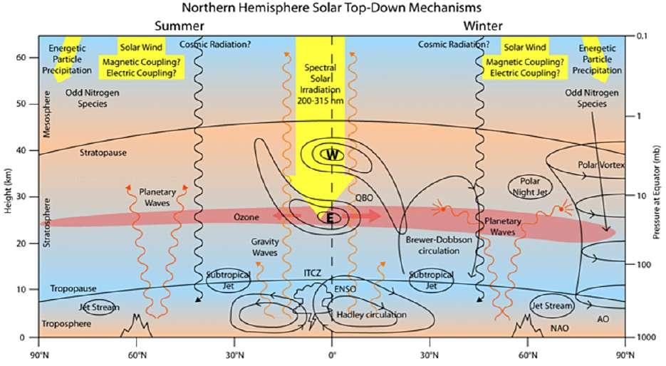
Figure 59. Summary of proposed top-down solar variability effects on climate. Only the Northern Hemisphere is represented, with the left and right halves showing the differences between summer and winter. The ITCZ, the Inter-Tropical Convergence Zone, is the climatic equator, ENSO, El Niño Southern Oscillation. Source: Javier (2018a).

Baldwin et al. (2001) explain “Most of this zonal momentum is deposited at stratospheric levels, driving the zonal wind anomalies of the QBO. Some gravity waves propagate through the entire stratosphere and produce a QBO near the mesopause known as the mesospheric QBO, or MQBO”. In the tropical lower stratosphere are represented the actual winds during the easterly phase of the QBO (In blue with symbol E) whereas at high latitudes, there is a pronounced annual cycle, with strong westerly winds during the winter season. During the easterly phase of the QBO the polar vortex north of ~45°N shows weaker westerly winds and the high-latitude wind anomalies penetrate the troposphere and provide a mechanism for the QBO to influence the tropospheric weather patterns and therefore as explained by Javier (2018a) “One of the most puzzling aspects of the QBO is that it also modulates the Northern Hemisphere Polar Vortex, a persistent, large-scale, midtroposphere to stratosphere, low pressure winter zone that when strong contains a large mass of very cold, dense Arctic air, and when weak and disorganized allows masses of cold Arctic air to push equatorward, causing sudden temperature drops in ample regions of the Northern Hemisphere”. Therefore, as visible on Figure 58 and 59, the QBO is originally a tropical phenomenon that by means of upward waves affects in the end the

191https://en.wikipedia.org/wiki/Rossby_wave - Carl-Gustaf Arvid Rossby first identified such waves in the Earth's atmosphere in 1939 and went on to explain their motion.

global stratosphere through the modulation of winds, temperatures, extra-tropical waves, meridional wind circulation, the transport of chemical constituents, and the repartition of ozone.

Labitzke and Van Loon (1988, 1989, 1991) and Van Loon and Labitzke (1988, 1990) had the idea to separate the data on stratospheric temperatures at the different latitudes according to the QBO phase (Kerr, 1987) and managed in that way to identify an obvious correlation with the solar cycles “Linear correlations between the three solar cycles in the period 1956–1987 and high-latitude stratospheric temperatures and geopotential heights show no associations. However, when the data are stratified according to the east or west phase of the Quasi-Biennial Oscillation (QBO) in the equatorial stratosphere significant correlations result: when the QBO was in its west phase the polar data were positively correlated with the solar cycle while those in middle and low latitudes were negatively correlated. The converse holds for the east phase of the QBO. Marked relationships existed throughout the troposphere too”. (Labitzke and Van Loon, 1988).

Not going to far, one can easily sense from what has been exposed now, that it is not trustworthy to claim on the basis of the sole short time-series of instrumental measures of the TSI that solar variations and cycles have to be dismissed as a major explanation of climate change. For example Labitzke states “But there is general agreement that the direct influence of the changes in the UV part of the solar spectrum (6 to 8% between solar maxima and minima) leads to more ozone and warming in the upper stratosphere (around 50 km) in solar maxima. This leads to changes in the vertical gradients and thus in the wind systems, which in turn lead to changes in the vertical propagation of the planetary waves that drive the global circulation. Therefore, the relatively weak, direct radiative forcing of the solar cycle in the stratosphere can lead to a large indirect dynamical response in the lower atmosphere.” This, it just demonstrates a will to jump to a foregone conclusion, which in the end is not too surprising given the one-sided mission of IPCC, demonstrate that climate-change is man(n)-made.

In a remarkable series of paper published on J. Curry “Climate Etc” website, Javier (2016a-b, 2017a-b-c-d-e-f-g, 2018a-bc-d) has covered most of the aspect of the climate over the Holocene. The above Figure 59 is from Javier (2018a) and summarizes the components we have briefly discussed and which play a role in responding to the solar action.

One will notice that the effects of solar wind or induced magnetic and/or electric coupling and the effects of cosmic rays are considered by Javier (2018a) as still quite unknown and they have been left out of Figure 59. This is a very cautionary stance as we have seen that more and more research work has proven the interactions happening between the solar wind, the magnetosphere and thereon from the stratosphere down to the troposphere, in the end impacting the Earth's cloud cover and thereof its albedo (e.g. Asikainen et al., 2017; Svensmark et al., 2016, 2017; Maliniemi 2016; Maliniemi et al., 2017). Depending on the phase of the solar cycle, electrons from tens to hundreds of keV, precipitate down to the mesosphere and upper stratosphere, where they can create nitrogen and hydrogen oxides which during winter time survive longer and can descend down to the mid-stratosphere and destroy ozone (Kilifarska and Haigh, 2003), which leads to cooling of the high-latitude stratosphere. This enhances the meridional temperature gradient and westerly winds, thus accelerating the polar vortex and leading to an anomalously positive Northern Annular Mode (NAM) which encloses the cold arctic air into the polar region and enhances the westerly winds at mid-latitudes 192 and Asikainen et al. (2017) assert “These results give additional evidence that not only solar electromagnetic radiation but also the solar wind can affect the climate”.

Javier (2018a) summarizes all the phenomenons displayed on Figure 59 “Energetic particle precipitation at the pole produces odd Nitrogen and Hydrogen species in the upper atmosphere, that are more efficiently transported downward by the winter stratospheric vortex, reducing polar ozone levels. UV solar irradiation, variable with the solar cycle, is responsible for the ozone layer and its temperature gradients. Different types of tropical waves (orange) originating from convection, are responsible for the creation and maintenance of the Quasi-Biennial Oscillation (QBO), that together with the Brewer-Dobson circulation193 is responsible for the poleward transport of ozone. The position of the Tropical Jet Stream is determined by the Hadley circulation, while the strength and position of the Jet Stream and the Polar Night Jet depend on the strength of the Polar Vortex. Depending on stratospheric conditions, planetary-scale Rossby waves (red) can be deflected during the winter, causing stratospheric warming and a weakening of the Polar

192Enhancement of westerlies brings warm and moist air from Atlantic to the Northern Eurasia causing positive temperature anomalies and at the same time negative temperature anomalies are observed in the Northern Canada and Greenland. 193Proposed by Alan Brewer in 1949 and Gordon Dobson in 1956, explains why tropical air has less ozone than polar air, even though the tropical stratosphere is where most atmospheric ozone is produced. It posits the existence of a slow current in the winter hemisphere which redistributes air from the tropics to the extra-tropics. The Brewer–Dobson circulation is driven by atmospheric waves.

Vortex. The Polar Vortex determines the winter state of the Arctic Oscillation (AO), which strongly influences the North Atlantic Oscillation (NAO). Solar activity level, through its effect on stratospheric conditions, influences Northern Hemisphere winter weather far more than its small change in irradiation suggests”, (bold added).

These planetary waves are well known by the meteorologists as they lead to strong temperature anomalies and major weather patterns, e.g. (Mann, 2019). How could climate, which is the sum (i.e. integral) over time of the weather, not be influenced by these complex relationships happening between the magnetosphere, the stratosphere, and the troposphere, not be influenced by them? Numerous physiochemical interactions happen in the stratosphere, some originating as high as the mesosphere and move down as waves impacting the tropopause and further propagate into the troposphere. These mechanisms were already envisaged by Stott et al. (2003) though more focused in that respect in their paper on UV interaction “Potentially the largest amplification of solar forcing could result from modulation of stratospheric ozone by variations in solar ultraviolet, which could influence the troposphere via modulation of planetary waves (Shindell et al. 1999) or modulation of the Hadley circulation (Haigh 1996)”.

These authors also remind us that the interplanetary magnetic field increased during the twentieth century and led to a decline of the intensity of CRF which contributed to increasing the solar effects on climate. Similar conclusions are drawn by Haigh and Blackburn (2006) “We conclude that solar heating of the stratosphere may produce changes in the circulation of the troposphere even without any direct forcing below the tropopause. We suggest that the impact of the stratospheric changes on wave propagation is key to the mechanisms involved”. GCM models have been pretty unable, even over extremely short-time scales (e.g. 11-year solar cycle) to render this troposphere-stratosphere coupling and especially to account for the the secondary maximum in temperature in the lower stratosphere. As pointed out by Gray et al. (2005) “This secondary maximum is likely to be an important part of the mechanism that transfers the solar signal from the lower stratosphere to the troposphere underestimate the ozone signal in the upper stratosphere / lower mesosphere”. One must acknowledge that we have very complex non-linear coupled-systems, e.g. (Simpson et al., 2009), and that the weather is clearly originating far from us as gravitational interactions modulate the Sun activity and cycles, the solar wind and charged particles play their role and one cannot just measure TSI variations over short instrumental periods to grasp how the Sun influences the weather and therefore over time the climate system.

Finally, Scafetta (2014) gives the big picture “It seems simply unlikely that in a solar system where everything appears more or less synchronized with everything else, only the Sun should not be synchronized in some complex way with planetary motion. Thus, the Earth’s climate could be modulated by a complex harmonic forcing consisting of (1) lunar tidal oscillations acting mostly in the ocean; (2) planetary-induced solar luminosity and electromagnetic oscillations modulating mostly the cloud cover, and therefore the Earth’s albedo; and (3) a gravitational synchronization with the Moon and other planets of the solar system modulating, for example, the Earth’s orbital trajectory and its length of day (cf. Mörner, 2013).”

As a side note, one should consider that even though the Earth’s climate has changed a lot on all timescales for various reasons that we have addressed, the strange couple that the Earth and the Moon form, the latter being abnormally large of a satellite with respect to Earth’s size, has lead to stabilizing the inclination of the Earth’s rotation axis on the ecliptic (tilt of the earth's axis relative to its orbit around the sun). This is a unique case in the solar system and very fortunate, as Mars for example which present a comparable inclination today to that of the Earth has seen its value change a lot over time (Touma and Wisdom, 1993). This has resulted in a much more stable climate on Earth than it would have been if the Moon hadn't teamed up with us (Ward and Brownlee, 2000).