3)Sea Level Changes

“The slow emergence of fossil fuel emissions prior to 1950 did not contribute significantly to 19th and early 20th century sea level rise. Identifying a potential human fingerprint on recent sea level rise is confounded by the large magnitude of natural internal variability associated with ocean circulation patterns. There is not yet any convincing evidence of such a fingerprint on sea level rise associated with human-caused global warming.” (Curry, 2018)

Rasool and Schneider (1971) had forecast that the increased rate of injection of man-made particulate matter in the atmosphere would return us in the next 50 years into an ice age. In the same paper, they noted though that « Even for an increase in CO2 by a factor of 10, the temperature increase does not exceed 2.5 °K. Therefore, the runaway greenhouse effect does not occur because the 15-µm CO2 band, which is the main source of absorption, "saturates," and the addition of more CO2 does not substantially increase the infrared opacity of the atmosphere». Both assertions were correct, though the ineluctable return to an ice age will not happen on short notice and not for the reasons given. They probably quickly sensed that their career needed a U turn to take some momentum and they converted to the rising tide of climate global warming alarmists. As soon as the late seventies, Schneider in the "The Palm Beach Post" edition of the 8th of January 1979, while working for the National Center for Atmospheric Research at Boulder (Colorado) predicted that «man-caused global warming would thus melt polar ice and raise sea levels by many feet ". Schneider predicted this as a possibility to happen before the end of this century (understand before 1999) and teamed up with Robert Chen of MIT to add «sea-level rise of 15 to 25-foot. The nation's coastline would change markedly».

Fifty years after these predictions failed miserably, it is therefore simply amazing to see the same scare tactics used again and again. Prophets of doom keep popping all over the place and litter the greatest universities worldwide and are ready to embark us on an economic Armageddon on baseless fears. Consider this example, of which we just pick-up one amazing sentence, as it cannot be further away from any decent scientific approach «One issue that concerns many scientists is that many of global warming's impacts have unfolded significantly faster than expected. For example, in 2007 the IPCC projected that global average sea levels would rise 0.6 meters (2 feet) by 2100, but in 2013 the prediction was revised to as much as 0.98 meters (3.2 feet), and then in 2016 revised again up to 2 meters (6.6 feet) » (Henderson et al., 2017). This is typical of the way people confuse astrological predictions through a crystal ball and how science should be made. So far, nothing has unfolded at all, the only thing that has happened is that changing the crystal ball they use, those charlatans have increased their «forecasts», but why not increase them to more than 20 meters, or even more to engineer a good epicontinental transgression? This analysis reported by Henderson et al. (2017) is based on a journalist paper (Jones, 2013).

In fact the conclusion of Jones’s (2013) paper is just hilarious; she quotes Don Chambers (sea level researcher at the University of Texas), who declares “I always tell people if they live under 3 feet above sea level, they should be worried about the next 100 years”, do you really think that these people will not have anything else to worry about for their next 100 years! Those academics simply live on another planet than the average Joe and do not even know it. The Henderson et al. (2017) paper continue «At the highest level, several studies suggest that the cost of mitigating the effects of climate change are likely to be much lower than the costs of leaving it unchecked. For example, the IPCC estimated that... leaving global warming unchecked might cost 23% to 74% of global per capita GDP by 2100…» What an accurate forecast that we must trust, between 23% to 74% of global per capita GDP, it is an amazing number and a dazing uncertainty, it is not even an astrological forecast any longer now but plain delirium. Then the ranting goes on by attempting to calculate «the social cost of carbon" (SCC), a measure designed to capture the economic damages caused by carbon emission...».

It is plain madness, there is no costs but only benefits to making use of carbon-based energies, they will strengthen the growth of plants and vegetables and they will enable us to keep achieving what humankind has made it possible to happen, a better life for everybody, as since the year 1500 human population has increased 14-fold, production 240fold and energy consumption 115-fold. It is because we have access to fossil and nuclear energy that we have increased production 240-fold. Academic staff from Harvard Business School are not just mistaken in their strange reasoning, they have gone straight into the ditch of non-sense. It is also amazing to see how lightly business academics can take numbers which are no better than what a roll of dice would give and claim « global warming's impacts have unfolded significantly faster than expected»!

Had they done their homework, not science as its not their job, they would have found that it takes 360 Gt of water to raise the sea level by 1 mm. Floating sea ice does not contribute to a Sea Level Rise (SLR). Tide gauges spread over the globe say that we have had a rise of around 1.3 mm/year (Wöppelmann et al., 2007) after GPS correction of the subsidence or the emergence of the basement carrying the tide gauge; a part (half?) of this 1.3 mm/year is attributed to a pumping of groundwater greater than their filling (local subsidence) and perhaps and for at most 0.5 mm - and for the last decade only - to a decrease of altitude glaciers outside Antarctica and Greenland. Altimeter observations (Zwally et al., 2012; 2015) suggest an Antarctic mass gain of 43 to 49 Gt-water/year revised upward in 2015 for 1992 to 2008 to +200 Gt-water / year on the eastern part and - 65 Gt-water/year on the western part and the Antarctic Peninsula, that is, net, 135 Gt-C / year sequestered.

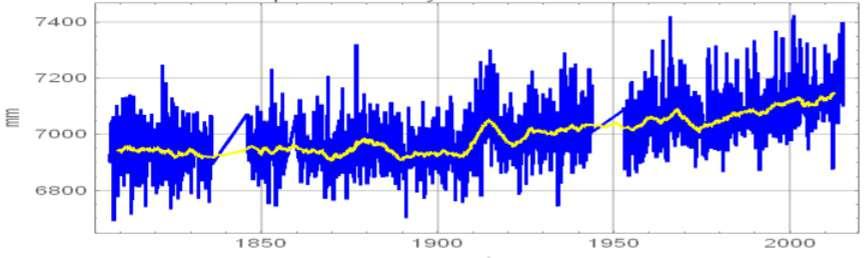
Figure 60. Average monthly levels in Brest since 1807: the big maximums are in Dec. 1821 (7225 mm), Nov. 1852 (7233 mm), Dec. 1876 (7322 mm), Feb. 1966 (7422 mm) and Dec. 2000 (7426 mm). The 18.6-year lunar cycle is visible on the annual averages while the monthly values mainly show the effect of winter storms. In yellow moving average over 5 years. http://www.psmsl.org/data/obtaining/rlr.monthly.data/1.rlrdata

Veyres (2020) reminds us that the longest series of monthly averages, the number 1 in the collection of the permanent sea level observation service (www.psmsl.org), that of Brest (France), Figure 60, shows an increase of +200mm in 207 years and +150mm over 1910-2015. So, none can say «the global warming's impacts have unfolded significantly faster than expected» as Henderson et al. (2017) claim, forecasts announcing a sea level rise of 2 meters by 2100 are just ridiculous, and observations show that so far over 207 years we have observed +200 mm, e.g. Church and White (2006) report 195 mm from January 1870 to December 2004, a tenth of what the doom-sayers claim over a much longer period than the 80 years to go until 2100! Furthermore, the Antarctic Peninsula, is sequestering net, 135 Gt-C/year and contribute to a decrease of the sea level of 0.375mm/year (Zwally et al., 2012; 2015). One of the objections some people have aired with our reasoning has been why don’t you use more global satellite data? The reason why we have been cautious with satellite data is that are constantly being reprocessed, adjusted, forged?, as it has been too often the case for other global observation data, for which obtaining «raw data» is always a challenge as these are too often locked down by the institutions managing them. This cast a doubt on their validity and makes their integrity questionable and this is unfortunate because this was not the case in the 1980s when the remote-sensing laboratory194 I used to work for made a daily usage of them in trust, before the climate fiasco and related hysteria.

This is not the case with sea gauges and whatever the world area where we get their data from, they show a coherent (across series) and consistent (over time and for Brest, long periods of time) picture : the sea level rise is minimum and there is no measurable significant acceleration: “It is evident that the installation of GPS equipment in 2000 has had an influence on stabilizing the SEAFRAME gauges. Since that date, there has been little evidence that the sea level is changing in the 12 Pacific islands” (Gray, 2010)195 or consider the report by Mitchell et al. (2012), i.e. South Pacific Sea Level and Climate Monitoring Project: Sea Level Data Summary Report, July 2010 to June 2011, and go to Fig. 10. Monthly mean sea levels 1991 to June 2011, p. 22, and you will see no sea-level rise for entire pacific area considered, flat curves (except perhaps the Federated States of Micronesia which has shorter time-serie and may be victim to subsidence). Furthermore, superimposed on the long-term searched-for eventual acceleration are quasi periodic fluctuations with a period of about 60 years (Figure 54) and the decadal variations of sea level dominate the estimate of acceleration for records shorter than about 75 years (Douglas, 1992; Jevrejeva et al., 2008).

194Centre de Télédétection et d'Analyse des Milieux Naturels (CTAMN) à Sophia Antipolis. http://www.oie.mines-paristech.fr/Accueil/Historique/ 195In memoriam of the fight for honesty https://en.wikipedia.org/wiki/Vincent_R._Gray

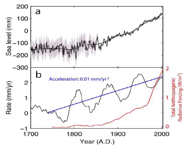
Figure 61. a) Time series of yearly global sea level calculated from 1023 tide gauge records corrected for local datum changes and glacial isostatic adjustment. Time variable trend detected by Monte-Carlo-Singular Spectrum Analysis with 30-year windows. Grey shading represents the standard errors. b) The evolution of the rate of the trend (black line) showing multidecadal variability. Blue line corresponds to the linear background sea level acceleration that corresponds to a sea level acceleration of 0.01 mm/yr2. Red line, IPCC calculated total anthropogenic radiative forcing. Source: Jevrejeva et al. (2008).

As reported by Douglas (1992) the acceleration can even be a deceleration as “for the 80‐year period 1905–1985, 23 essentially complete tide gauge records in 10 geographic groups are available for analysis. These yielded the apparent global acceleration −0.011 (±0.012) mm/yr2”. Whatever the data analyzed by Houston and Dean (2011), using leastsquares quadratic analysis of tide gauges provided either by the Permanent Service for Mean Sea Level (PSMSL), or Douglas (1992), or Church and White (2006), they obtain small average sea-level decelerations. As displayed on the previous Figure 61 from Jevrejeva et al. (2008), SLR started more than 200 years ago, when anthropic emission were ridiculously small as displayed by the red curve in b). The central estimate on 20th-century average SLR is ~ 1.6 mm/yr (1.2-1.9 mm/yr range), and the acceleration d(SLR)/dt is usually estimated as small as ~0.01 mm/yr 2 ! “A reconstruction of global sea level since 1700 has been made. Results from the analysis of a 300 year long global sea level using two different methods provide evidence that global sea level acceleration up to the present has been about 0.01 mm/yr 2 and appears to have started at the end of the 18th century” (Jevrejeva et al. 2008).

SLR displays a 60-year oscillation, like many other climatic manifestations. The recent period of satellite altimetry (1993-2017) coincides with the crest of the oscillation, and thus shows a higher rate of SLR, ~ 3.0 mm/yr, but no acceleration, to the surprise of some authors: “Global mean sea level rise estimated from satellite altimetry provides a strong constraint on climate variability and change and is expected to accelerate as the rates of both ocean warming and cryospheric mass loss increase over time. In stark contrast to this expectation however, current altimeter products show the rate of sea level rise to have decreased from the first to second decades of the altimeter era” (Fasullo et al., 2016). The conclusion here is given by Javier (2018) “If the 60-year oscillation continues affecting SLR, over the next couple of decades we should expect a deceleration of SLR rates towards ~2 mm/yr”.

As was the case with temperature, SLR precedes the big increase in emissions, and does not respond perceptibly to the anthropogenic contribution. The b) graph of the previous Figure 61 displays the linearly adjusted trend in long term average SLR acceleration as a blue line, and the increase in anthropogenic “forcing” (IPCC-AR5, 2013) with a red line. The evidence shows that the big increase in anthropogenic contribution, has not provoked any perceptible effect on SLR acceleration. “The belief that a decrease in our emissions should affect the rate of SLR has no basis in the evidence” (Javier, 2018b). The observed SLR is the result of the cryosphere response to the warming that started since the end of LIA and no proof can be given that a significant acceleration (so far observed at ~0.01 mm/yr2) is to be expected.

This had to be acknowledged by Fasullo et al., (2016) who expected that satellite altimetry would save their day. When an acceleration is shown it is mostly caused by selective trend calculation (i.e. cherry-picking). For example, by using a

start year of 1993, at the bottom of a dip in the trend, a spurious calculation of 3.1 mm/yr is obtained instead of 1.6 mm/yr. In reality the recent data is in line with the long-term trend and the “acceleration” is artificial. Sea level reconstructions over longer terms, such as those performed by Grinsted et al. (2009) show that thermo-steric expansion (Domingues et al., 2008), (Purkey et al., 2014), (Madec et al., 2015) explains a part of variations observed “Over the last 2000 years minimum sea level (-19 to -26 cm) occurred around 1730 AD, maximum sea level (12 to 21 cm) around 1150 AD”, therefore the high corresponds to the MWP and the low to the LIA and gives a clear idea of the amplitude of the variations that one can expect from the current on-going natural warming that took place since the end of the LIA. It also clearly shows the correspondence with MWP and LIA which were removed of climate reconstructions by Mann and IPCC.

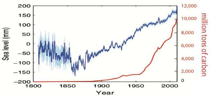
Figure 62. Time series of sea level anomalies (blue) Jevrejeva et al. (2014). Million tons of carbon emitted from burning fossil fuels (red) from the Carbon Dioxide Information Analysis Center (CDIAC 2014). Source: (Curry, 2018). As one can see there is simply no relationship, SLR (blue) started long before significant anthropogenic emissions and did not accelerate with the massive increase of emissions since the late 1950s. Another culprit will have to be found.

These facts are highlighted by Curry (2018) “At least in some regions, sea level was higher than present around 5000 to 7000 years ago. After several centuries of sea level decline following the Medieval Warm Period, sea levels began to rise in the mid 19th century. Rates of global mean sea level rise between 1920 and 1950 were comparable to recent rates. It is concluded that recent change is within the range of natural sea level variability over the past several thousand years”.

Furthermore, recent studies show (Fudge et al., 2016) that there is no straightforward and durable relationship between the temperature and the ice accumulation rate at the poles and that, of course, prevents from making any decent forecast to an SLR contribution. In fact, The Antarctic and or Arctic contribution to sea level is a balance between ice loss along the margin and accumulation in the interior. But in Antarctic, at least as far as the WAIS Divide (WDC) site is concerned, and over the 31 kyr studied with high resolution recently, results show considerable variability through time with high correlation and high sensitivity (between temperature and accumulation) for the 0–8 kyr period but no correlation for the 8–15 kyr period and then Fudge et al. (2016) report: “Accumulation records for the past few decades are noisy and show inconsistent relationships with temperature. These results suggest that variations in atmospheric circulation are an important driver of Antarctic accumulation but they are not adequately captured in model simulations. Model-based projections of future Antarctic accumulation, and its impact on sea level, should be treated with caution”.

Basically, the General Circulation Models are simply unable to account for the 15 most recent kyr and corresponding estimates of SLR contribution are fictions as there does not even exist a stable relationship between the temperature and ice accumulation rates. If Antarctic is in no way significantly a contributor to any SLR, one can reliably assess that Arctic has been a net contributor since the switch of its the decadal mass balance which occurred in between 1972–1980 when showed a mass gain of +47 ± 21 Gt/y and tilted to a loss of 51 ± 17 Gt/y in 1980–1990 (Mouginot et al., 2019). Cumulated since 1972, these authors report that Arctic has been the main contributor to SLR, i.e. “ the largest contributions to global sea level rise are from northwest (4.4 ± 0.2 mm), southeast (3.0 ± 0.3 mm), and central west (2.0 ± 0.2 mm) Greenland, with a total 13.7 ± 1.1 mm for the ice sheet. The mass loss is controlled at 66 ± 8% by glacier dynamics (9.1 mm) and 34 ± 8% by SMB196 (4.6 mm)”, but will see in the section dealing with the Arctic that it is in no way outside of normal natural variability.

196SMB = Surface Mass Balance

Then people can run computer models or throw the dice to try to scare the public, the result is not very different. In that respect, Storch et al. (2008) considered as experts in that domain have studied the relationship between global mean sea-level and global mean temperature in a climate simulation of the past millennium and are honest when they report that «it has been found that the best statistical model of the four explored here is the one that uses the ocean heat-flux as predictor. Unfortunately, the ocean heat-flux is a variable that is difficult to estimate in the real world, and of which long time series simply do not exist. Therefore, this close relationship is not useful to estimate empirically future sea-level changes. The linear link between global mean temperature and the rate of change of global mean sea level (model Eq. 1) has turned out to be not reliable over the full time period in the context of this climate simulation; instead, for some periods, even inverse relationships were found to describe the simulated data best. The second predictor “rate of change of temperature”, used in model Eq. 4, analyzed here in more detail, did not show markedly better results. For both predictors, there exist periods in the simulation where the prediction errors are very large ». Basically, running sophisticated computer models, in that case four different, has not delivered any reliable estimate of what the sea level rise could be, instead sometimes providing even inverse relationships!

Furthermore, trying to attribute to anthropogenic CO2 emissions SLR will be made extremely difficult by the natural, internal climate variability associated with ocean circulations, i.e. currents and winds. These introduce strong changes in regional sea level on timescales from years to decades (and even longer). As reported by Curry (2018) “For example, sea level variability in the Pacific Ocean related to El Niño Southern Oscillation (ENSO) and to the Pacific Decadal Oscillation (PDO) is of the order of ±10–20 cm, which masks any sea level changes due to increasing CO2”.

Finally all geologists know that a level is highly variable as the land used as a reference can instead experience subsidence or rise for various geodynamic reasons, one of the most frequent being just an isostatic adjustment, example taken by Legates in his testimony “Sea level, while important to areas in southeastern Pennsylvania along the Delaware River, has risen steadily over the past 120 years but shows no correlation with increasing carbon dioxide concentrations. At the US Coast Guard Station in Philadelphia, sea level is likely to rise another 9½ inches by 2100, but half of that rise in sea level is due to coastal subsidence due to Glacial Isostatic Adjustment from the unloading of glacial ice since the last Ice Age some 22,000 years ago” (Legates, 2019).

The main cause of U.S. East Coast subsidence is natural and is due to the melting of the ice-sheet that covered northern America during the LGM. The land beneath it has been springing back up by isostatic adjustment and like a see-saw, that's causing areas south of the former ice sheet to sink back down, including Maryland, Virginia and North Carolina. Other areas have experienced strong subsidence mechanisms leading to an apparent sea level rise, and e.g., Nienhuis et al. (2017) report “Coastal Louisiana has experienced catastrophic rates of wetland loss over the past century, equivalent in area to the state of Delaware. Land subsidence in the absence of rapid accretion is one of the key drivers of wetland loss”.

What is serious, is that Harvard Business School academics should not jump start on the first scare and realize that major economic disruptions will happen if people keep going along IPCC’s line of thoughts without doing their own homework and cross-checking of data and results. So, nobody can claim that he knows where the sea level will be in 2100, not the IPCC better than others as they have consistently been wrong with all their predictions, but what I am sure about is that given the complexity of the subject, the fuzziness of the forecasts and the limited understanding we have of the situation, we are going to face many other problems, more worrying, before that one might happen in 2100, if it will, especially if we destroy our economies for such kind of non-sense and disrupt our industries and create massive poverty and unemployment. I would suggest that business schools focus on improving businesses, productivity and wealth creation and not worry about where the sea level will be in 2100 and do not take whimsical predictions for granted.

“In many of the most vulnerable coastal locations, the dominant causes of local sea level rise problems are natural oceanic and geologic processes and land use practices. Land use and coastal engineering in the major coastal cities have brought on many of the worst local problems, notably landfilling in coastal wetland areas and groundwater extraction” (Curry, 2018)

It is not possible to close this short section on “sea level rise” without mentioning the work of Nils-Axel Mörner who passed away on Oct 16, 2020. As summarized by Monckton of Brenchley (2020c) “he knew more about sea level than did Poseidon himself. Professor Mörner was a hands-on scientist. He did not enjoy squatting in his ivory tower. He liked to travel the world investigating sea level by the novel method of actually going to the coastline and having a look”. Mörner wrote many papers on the subject with the rigor of a great scientist, a great geologist who always put more

credence on the facts observed in situ than on any other remote measurements, such as data acquired by satellites. This sounds like the basics of natural sciences, go into the field, observe things as they are, not running sea-level change models on computers and dismissing what's visible in plain sight! By doing so, he was involved in many projects with a host of scientists who welcomed him in distant parts of the world, such as the in the Maldives Project (2000-2005) , in the Qatar Project (2006), in the Bangladesh Project (2009), in the Goa Project (2013), and in the Fiji Project (2017). In Mörner (2017) he observes that because the satellite altimetry data have been “corrected” to give a rise in the order of 3.0 mm/yr the value of the observations in the field is paramount. Mörner (2017) notes “This 'correction' may, of course, be classified as a “manipulation” of facts, like the manipulation temperature measurements recently revealed ” making reference to the tortuous issue raised by Rose (2017a-b). He concludes “In this situation, there are all reasons to return to solid observational facts. Those facts are controllable, and this is a key criterion in science. The global perspective is general stability to a minor rise with variations between ±0.0 and +1.0 mm/yr. This poses no problem for coastal protection”. Other studies worth reading are (Mörner, 2010-2011, 2012).

His studies in all the places he visited confirm the very slow SLR that have been reported here, that occur since the end of LIA, and show no acceleration whatsoever as visible on Figure 62, whereas the emissions have kept growing at an accelerated rate. He even reported in some places as in Bangladesh that the sea level was actually falling and that when locally some anomalies occurred, they were related to completely different reasons, e.g. local prawn farmers had grubbed up the mangroves whose roots had previously kept the coastline stable. As reported by Monckton of Brenchley (2020c) in Mörner's eulogy “On another occasion Professor Mörner was visiting the Maldives when he noticed a small tree, 40 years old, right on the beach, in leaf but lying on its side. The fact that the tree was still there, feet from the ocean and inches above sea level, after 40 years told him that there had been no sea-level rise since the tree had first begun to grow, or it would have been drowned. He enquired locally about whether there had been an exceptional spring tide caused by global warming and sea-level rise that had overthrown the tree. He discovered, however, that a group of Australian environmental extremists had visited the beach shortly before him. They had realized that the presence of the tree showed that the official sea-level record showing a sharp rise over the past halfcentury must be incorrect, and had uprooted the tree. Professor Mörner stood it back up again and photographed it.”

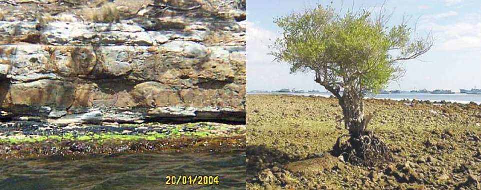
Figure 63. Left: The V atop an horizontal bar Ɣ197 visible inside the ellipse (near center-left) which stands a bit less than one meter above the water is a mark 50 cm across (tidal range is less than a meter) that was etched by Capt. Sir James Clark Ross in 1841 to indicate the mean sea level and is still perfectly visible in this picture made by Daly in 2004 at the Isle of the Dead (Tasmania) showing that no significant SLR has occurred since 1841, < 0.8±0.2 mm/yr as per Hunter et al. (2003), Fig. 1 and 2, p.54-2 and 54-3, for the complete story refuting the SLR altogether, see Daly (2003a-b-c). Right: the Mörner Tree of the Knowledge of Good and Evil shows that no SLR occurred either in the Maldives, from Monckton of Brenchley (2020c).

Exactly as the picture taken by John L. Daly in 2004 (low tide on 20 Jan.) of the 1841 sea level benchmark (inside the ellipse) on the `Isle of the Dead'198, Tasmania, remains and reminds where was, according to Antarctic explorer Capt. Sir James Clark Ross, the mean sea level in 1841 (Ross, 1847), the Mörner Tree of the Knowledge of Good and Evil199

197Go to http://www.john-daly.com/photomrk.htm for a larger picture. 198https://en.wikipedia.org/wiki/Isle_of_the_Dead_(Tasmania) 199https://en.wikipedia.org/wiki/Tree_of_the_knowledge_of_good_and_evil

should lead to the expulsion of all the cheaters, the manipulators, the unworthy ones from the realm of science. These are facts rooted in the field observations, not on 'corrected', i.e. fudged? satellite data and fantasy computer models. They are also completely at odds with statements in the press made by Mann and Hansen (Wallace-Wells, 2017), who appear more as climate activists and alarmists than as scientists in such operations of intentional deception (see p. 321).

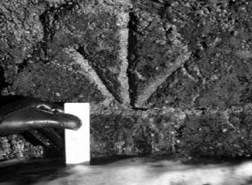
Figure 64. Zoom on the etched benchmark displayed in the ellipse (near center-left) of Figure 63, that was engraved under the order of Capt. Sir James Clark Ross in 1841 to indicate the mean sea level at the Isle of the Dead (Tasmania). After Hunter et al. (2003).

The mark carved by Lempriere under the instructions of Ross (Figure 64) has led to a dispute between Daly (2003a-b-c) and Hunter et al. (2003) who write “From the position of the benchmark relative to mean sea level as estimated in 1875– 1905, 1888 and 1972, and from our modern records (Figure 2), we believe that it is inconceivable that the benchmark could have been at mean sea level in 1841”. It can be inconceivable for them, but it is what Ross (1847) stated in several occasions and wrote in his book “The fixing of solid and well secured marks for the purpose of showing the mean level of the ocean at a given epoch, was suggested by Baron von Humboldt, in a letter to Lord Minto, subsequent to the sailing of the expedition, and of which I did not receive any account until our return from the Antarctic seas, which is the reason of my not having established a similar mark on the rocks of Kerguelen Island, or some part of the shores of Victoria Land. ...". From thereof is rooted the origin of the disagreement with Daly (2003a-bc) the importance of which is further minimized by Hunter et al. (2003) stating that this single point would not alter significantly the global picture and the results of surveys based, e.g. on say 24 other stations (Douglas, 1997). This is of course true and incorrect at the same time: arithmetically true if one considers that Port Arthur, Tasmania, is just one observation point of a series of a well established theory this being the position of Hunter et al. (2003) and incorrect if one considers that one observation is more than enough to refute a theory as long as it is certain, which is Daly's (2003a-b-c) stance. The latter is especially true given the uniqueness of the engraving at the Isle of the Dead, delivering the oldest physical reference that provides for the longest direct observation of the sea-level. The situation is further complicated by the fact that the 1880s tremors may have changed the geographical setting at Port Arthur, Tasmania (and thus corresponding levels up or down, in fact as in many other places 200 for various geodynamical reasons such as tectonic or isostatic natural adjustments). These earthquakes were well documented by Shortt (1885) and reported on a map where appears the likely epicenter of a series of earth tremors (also listed in a comprehensive table) that occurred in Tasmania between 1883 and 1885, and which continued into 1886 after he published his paper. They were unprecedented in both scale and frequency either before or since.

The Isle of the Dead in Tasmania is certainly not the only place where the battle rages. The Maldive archipelago is also regularly used by the scare mongers to let people think of a supposedly urgency to take drastic measures to circumvent the alleged catastrophic SLR that should submerge the low lying islands worldwide. The only problem is that their apocalyptic vision does not match with the facts, the mere reality, when observed in a non-partisan way. This is just what Duvat (2020) did in her recent paper where it appears that since 2005, 110 (59.1%) of the 186 islands in the Maldives studied grew by ≥3%. Of those 110 expanding islands, 57 grew by ≥10% and 19 grew by ≥50%, that’s just in the last decade. Of the islands that didn’t expand in size, 38.2% (71 islands) were classified as stable (defined as neither growing or contracting by more than 3%). This leaves only 5 islands out of 186 (2.7%) that decreased in size since the 1980s. Put another way, 97.3% of Maldives islands have been either stable or growing since 2005, all while Climate Alarmists have exploited the Maldives as a poster child of ‘’sinking islands” to recruit gullible children into their cult.

200Recent vertical motions can be assessed using the following site: https://www.sonel.org/-GPS-.html CGPS indicates rising land motion for many places, e.g. Oslo, Norway and Vaasa, Finland, 5.33 +/- 1.12 mm/yr at Oslo and 7.88 +/- 1.14 mm/yr at Vaasa leading to sea-level drops!

This situation is despite the fact that the Maldives islands are objectively a region characterized as one of the most vulnerable to sea level rise perturbation, as about 80% of the islands are less than 1 meter (m) above sea level.

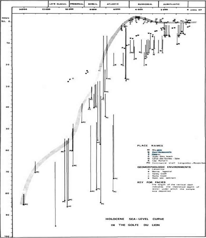
Figure 65. Sea-level change over the last 14.000 years (Holocene) in the “Golfe du Lion” as per Aloïsi et al. (1978) showing a constant SLR of +1mm/year over 8000 years, stopping at -4,500 years ago. This reconstruction matches that of Lambeck and Bard (2000), Fig. 3. Since the top observed at -4,000 the sea level has been pretty stable as reported by Morhange et al. (2001). After Aloïsi et al. (1978). See also O'Brien et al. (1995), Fig. 2 (center-down), p. 1963.

Considering that the Maldives population (>400,000) has been doubling every 25 years since the 1960s and nearly 1.3 million tourists visit many of the 188 inhabited islands every year, the Maldives islands are especially vulnerable and represent a landmark in the critical assessment of the effects of sea level change. The situation shows that if a small SLR has occurred, has it really?, it has been defeated by human ingenuity, adaptation to changing conditions being the best response as always, and engineering feats such as island raising, artificially expanding island areas, and “armoring” shorelines, have lead to an expansion of most of the Maldives in recent decades. Rightfully making a difference between the islands where man intervention and engineering led to human adaptation and “natural” islands, Duvat (2020) states “As a result of widespread human intervention, these islands behave very differently from both the documented Pacific islands and the Maldivian islands of Gaafu-Alifu Dhaalu Atoll (most of which are ‘natural’), 15.5 % and 19.5 % of which underwent expansion over the past decades, respectively”. The later islands, referred to as the Huvadhu atoll, is a large atoll that contains 255 extremely low lying islands, the most in the Maldives and is further divided in between the Northern Huvadhu Atoll (Gaafu Alifu), and Southern Huvadhu Atoll (Gaafu Dhaalu). So even in that extremely unfavorable case, nearly 20% of the islands managed to show some natural expansion which is, in itself, a bewildering observation. But in fact what Duvat and Magnan (2019) report is that it is the anthropogenic change

brought to these islands to accommodate population expansion or economic development that is the main factor behind island evolution and not any related climate-change problem and of course this drives what the adaptation strategies to any possible future climate-change should be as they differ for rather unadulterated ecosystems (Type 1 and 2 islands) and other islands' types. In any case, so far, it is certainly not the supposedly devastating AGW-related SLR that is driving the future of these atolls. Furthermore in a previous study, Duvat (2018) published a global assessment of how the Earth’s islands and atolls are faring against the ongoing challenge of sea level rise since satellite monitoring began in the 1980s. She reported “no widespread sign of physical destabilization in the face of sea-level rise.” In fact, a) none of the 30 atolls analyzed lost land area, b) 88.6% of the 709 islands studied were either stable or increased in area, c) no island larger than 10 hectare (ha) decreased in size, and d) only 4 of 334 islands (1.2%) larger than 5 ha had decreased in size. The rapidly increasing population ever drawing more of the local resources of these small low lying islands is creating a challenge to nature conservation and preservation, and is not related to supposedly AGW-induced climate change.

To better put this section in perspective, one should notice that transgressions and regressions are the very basics of a scientific discipline, i.e. stratigraphy and that they have happened constantly over millions or rather hundreds of million of years and are well documented by geologists. They have been constantly happening over the recent late PliocenePleistocene and have been extensively studied, e.g. (Brigham-Grette and Carter, 1992; Bromley and D'Alessandro, 1987; Malatesta and Zarlenga, 1988; Migoń and Goudie, 2012; Naish and Kamp, 1995; Yi, et al., 2016). During the Eemian the Mediterranean sea was up to 6 meters higher than now (Gilli, 2018). Just considering the very recent record, i.e. since the end of the LGM, 30,000 years ago, e.g. as per Lambeck and Bard (2000) or more accurately for the last 14,000 years as studied by Aloïsi et al. (1978), a marine transgression has been observed worldwide and many papers documented correctly what was in the geological record. The previous Figure 65 is from Aloïsi et al. (1978) and shows a 80 meters increase of the sea-level over the period -12.5ky to -4.5ky and a quasi stagnation since -4.5ky as can be attested by observations, e.g. in the Cosquer Cave201 (Collina-Girard, 2014). Basically a 10mm/year increase over 8,000 years corresponding to the end of the stadial (glacial stage). It is also known that during the MIS 5a the sea level was higher than that observed now and the timing of this ~84- to 80-kyr maximum closely matches the June 60°N insolation peak at ~84 kyr, see Dorale et al. (2010) Fig. 2. It also appears that the ice-sheets built up during the cold MIS 5b completely and very rapidly melted or so and that MIS 5a was thus warmer and more ice-free than now, while MIS 5a also nearly matches MIS 5e-1 (~117 kyr). These observations provide evidences of the strong natural variability over the last ~100 kyr, whereas changes of the atmospheric composition certainly did not drive it.

We have evidenced from Figure 60, that direct measurements since 1821 show that since the end of LIA (and with no relationship to man-made emissions) we have had a return to a transient regime of SLR. The end of the interglacial is in sight, in less than 1,000-1,500 years and things will naturally strongly reverse (marine regression). Don't we have more urgent problems to solve over the next millennium than a potential but absolutely uncertain 1 to 1.5 meter maximum sea-level rise before returning to an ice-age? Can't we adapt to that over a millennium? In many places in southern Italy, because of natural changes and tectonic adjustments many antic harbors (dating back to -2.000 years) are kilometers inside the lands or inversely submerged by natural subsidence. Did mankind stay there, people twiddling their thumbs waiting for catastrophic sea-level changes, either up or down ? In any case fossil fuels will have been exhausted centuries before then.

My understanding is that we argue again about measures which are unable to deliver a clear anthropogenic signal that would be undeniably different from the natural variability and as summarized by Figures 60, 61 and 62, there has been since the end of LIA a slow and rather steady SLR that did not show any meaningful acceleration whereas the CO 2 emissions have been skyrocketing since 1950 (to properly assess their effects one should of course take their logarithm, but nonetheless) and in any case adaptation and remediation would be better policies to cope with a phenomenon that started hundreds years ago from natural variations than to enact radical measures that most probably will have no effect on the natural order of the things and will harm severely the prosperity of humanity by restricting access to cheap and easily available energy sources, see e.g. (Lomborg, 2020a-b).

Finally as the melting of the poles cannot account for any significant SLR, the AGW-proponents have tried to find a solution into the thermo steric (see foot-note 460) expansion of the oceans. This required a new conjecture, that of the heat hidden in the oceans, which is one more lasting deception. Argo is an international program that uses a fleet of more than 4,000 profiling floats to observe temperature, salinity, currents, and, recently, bio-optical properties in the Earth's oceans; it has been operational since the early 2000s and is mainly used to monitor the Ocean Heat Content

201https://en.wikipedia.org/wiki/Cosquer_Cave by 43° 12′ 10″ N, 5° 26′ 57″ E

(OHC). Heat is an energy measured in Joules and it flows only from the warmer to the colder as Rudolf Clausius stated it in 1850 with the second principle of thermodynamics. One should observe here that if the IR properties of the water molecule explain why some heat re-emitted by the Earth is absorbed in the IR by water and water vapor in the atmosphere (the so called GH effect), it also explains why no IR radiation can penetrate the oceans for the simple reason that a few microns of water stop them due to the vibrations of the water molecule. By using data delivered by such a massive fleet of "Argo floats" Wunsch and Heimbach (2014) have analyzed the oceans down to the abyss and report an increase of 4 1022 Joules over a 19 years period, this apparently very large energy contributing to the radiative forcing of a tiny 0.2 W/m2, this value has steadily decreased over the years, from a max given by Hansen et al. (2005) of 0.8 W/m2, Lyman et al. (2010) of [0.53-0.75 W/m2], von Schuckmann et al. (2011) of 0.54±0.1 W/m2, down to 0.2 W/m2 by Wunsch and Heimbach (2014). Given the volume of the oceans of 1,3 1018 m3, thus a mass of 1,3 1018 tons, Wunsch and Heimbach (2014) have deduced a calorific capacity of 5.4 1024 Joules per degree °K.

As the mean temperature of the oceans is 15° ±13°C, i.e. 288 ±13°K, the thermal energy contained in the oceans is around 5.4 1024 x 288 = 1.5 1027 Joules and thus over 19 years the energy accumulated in the oceans is 19 x 1.5 10 27 Joules. Thus, the annual increase can be computed as (4 10 22) / (19 x 1.5 1027) = 0.00014%, and an annual warming of a very small amount: (4 1022) / (19 x 5.4 1024) = 0.0004°C/yr as detailed by Gervais (2018).

Such a ridiculously small number is beyond even ARGO system's measurements capabilities and is furthermore, if real, very heterogeneously distributed across the various oceanic basins. Again, these values when compared to the natural variability appear insignificant.

In the end, can we get a better proof to show that the subject is a propaganda issue, not a scientific one, than the fact that people like Al Gore and Susan Solomon (Co-Chair for Working Group I for the IPCC's Fourth Assessment Report) have invested heavily in beach-front properties, so worried they are of the threatening sea level rise to come.