5)Glaciers, Ice-Cores, Arctic and Antarctic

“Temperature measurements in the arctic suggest that it was just as warm there in the 1930's...before most greenhouse gas emissions. Don't you ever wonder whether sea ice concentrations back then were low, too?” Roy Spencer

As was detailed in the “Past Climates” section of this document and the corresponding sub-sections “The last 2,000 years” and “The last 12,000 years, brief overview of the Holocene”, glaciers offer a fast response to any climate change. Trutat's (1876) striking observations, made long before man-made emissions, were reported several times and they were not isolated (Nussbaumer et al., 2011; Fig. 4 and 5), this is why glaciers have often been an easy prey to the scare mongering tactics of climate fabricators, as they have been generally receding since the end of the LIA (Akasofu, 2011). In fact, one can regularly see such reports in mass media come to the cover or front-page of newspapers or magazines to create sort of a Pavlovian response of the conditioned masses, where the gullible and easy to influence people, because they lack the time, will or the wherewithals to reach an informed opinion, get an imprint in their mind that there is no arguing, worse no denying (with an implicit creepy hidden allusion to the holocaust), things are written, the mass is said, man-made global warming is irrefutable, glaciers will disappear.

The inconvenient reality is that even this easy gamble, yes they melt, has often been lost by the manipulators. It was already reported how the managers of Glacier National Park, a large wilderness area in Montana's Rocky Mountains, have had to remove signs stating that «glaciers will be gone by 2020» as nature did not want to cooperate with their dire predictions. This was not the first time that glaciers had been devious and contradicted lightly formulated forecasts. The leak of the Climatic Research Unit's (CRU) “Climategate209” emails from the University of East Anglia (UEA), as if not embarrassing enough, coincided with the exposure of some blatant errors in the IPCC AR4 report (IPCC, 2007a), most notably a claim that Himalayan glaciers would disappear by 2035, an affirmation that turned out to completely lack of any scientific basis, e.g. (Bagla, 2009), (Cogley, 2011) and led to a contorted apology of the Chair and Vice-Chairs of the IPCC, and the Co-Chairs of the IPCC Working Groups (IPCC, 2010). Senior glaciologist Vijay Kumar Raina, formerly of the Geological Survey of India, had to deny the unsubstantiated claims by IPCC by dismissing that measurements made of a handful of glaciers would be representative of the fate of India's 10,000 or so Himalayan glaciers and that they would be shrinking rapidly in response to climate change (Raina, 2009). The document, i.e. a “Discussion Paper, Ministry of Environment and Forests” is not available any longer on its original web site (electronic form of book burning?) but the Heartland Institute archives it. In it, Raina (2009) states “Glaciers in the Himalayas, over a period of the last 100 years, behave in contrasting ways... It is premature to make a statement that glaciers in the Himalayas are retreating abnormally because of the global warming. A glacier is affected by a range of physical features and a complex interplay of climatic factors. It is therefore unlikely that the snout movement of any glacier can be claimed to be a result of periodic climate variation until many centuries of observations become available. While glacier movements are primarily due to climate and snowfall, snout movements appear to be peculiar to each particular glacier” and in fact they “cooperate” so little that “one side of a glacier tongue may be advancing while the other is stagnant or even retreating” Raina (2009). Vijay Kumar Raina's is now former or ex- of all the positions he occupied and is identified as the author210 of a controversial discussion paper and tagged by desmog as a member of climate resistance211, an honor; imagine he had the gall to state “Climate changes naturally all the time, sometimes dramatically. The hypothesis that our emissions of CO2 have caused, or will cause, dangerous warming is not supported by the evidence”. Well, getting rid of him will not make Himalayan glacier melt faster, but many will probably have rejoiced of that nice catch.

IPCC acknowledged of the mistake in a statement dated 20th Jan 2010 where they stated “It has, however, recently come to our attention that a paragraph in the 938-page Working Group II contribution to the underlying assessment refers to poorly substantiated estimates of rate of recession and date for the disappearance of Himalayan glaciers” (IPCC, 2010). it's so awkward on the part of the IPCC to make use of an unsubstantiated WWF interview when then keep claiming that they only resort to peer-reviewed literature, which is no wonder as they control throughout their vast network of lead authors and affiliated scientists all the gates of official publications in their related domain, which is in itself a problem often stressed by dissident scientists who have been marginalized for not conforming with the dogma.

209https://www.conservapedia.com/index.php?title=Climategate 210https://en.wikipedia.org/wiki/Vijay_Kumar_Raina 211https://www.desmogblog.com/vijay-kumar-raina

In fact Raina (2013), given his extensive knowledge over decades of Himalayan glaciers, is even more cautious than the position that we could have defended. He does not even observe a rapid response of glacier to changing climate and says “So far as observation of the glaciers, for more than five decades now, allows a judgment, I have no hesitation in making a statement that a glacier does not necessarily respond to the immediate climatic changes. Data presented reveals the fact that the glacier snout fluctuation is not influenced by one single parameter but by a combination of parameters. Physiographic character of the accumulation zone and valley slope probably has more dominant role than the annual precipitation and the atmospheric temperature per se” (Raina, 2013).

Denying the evidence that glaciers had been melting long before any anthropogenic emission since the end of LIA, will not help either hiding that Hannibal's crossing with his elephants of the Alps during the Second Punic War, 218 BC was only possible because there was no glacier on his path nor of ice at the time, at the end of October. Controversy over the alpine route taken by the Hannibal's Army from the Rhône Basin into Italy in 218 BC (2,170 cal BP) has raged for over two millennia, but recently Mahaney et al. (2018) brought it to an end by confirming what Polybius 212 wrote, i.e. that Hannibal had crossed the highest of the Alpine passes: Col de la Traversette (2,947 meters!) between the upper Guil valley and the upper Po river is indeed the highest pass. It was the end of October, troops had been marching for over five months, when Hannibal ordered the descent to Italy and snowy weather was to welcome them. Furthermore, “Hannibal's Numidian cavalry carried on working on the road, taking three more days to fix it sufficiently to allow the elephants to cross to the plain” and three days later, the elephants – not exactly a high mountain animal – had managed in 218 BC to cross in autumn the highest pass of the Alps. This is of course a testimony of how much warmer conditions in 218 BC were than those encountered now-days even after two centuries of natural warming following the end of LIA, but it is probably far from the very warm conditions met there 7,000 BP as Joerin et al. (2006), standing in front of the Tschierva Glacier in Engadin, Switzerland at 2,200 meters (7,217 feet) reminds that 7,000 years ago they were no glacier at all "Back then we would have been standing in the middle of a forest".

The climate has kept changing a lot, with or without our ridiculous anthropogenic emissions, and for the time being, even the easiest wager of the climate fabricators is regularly lost. Even the Alaskan glaciers do not cooperate as expected and as reported by Berthier et al. (2010) previous studies have largely overestimated mass loss from Alaskan glaciers over the past 40-plus years. As reminded by Spencer (2007) glacier obviously do react to temperature changes but more importantly to precipitation changes “Similar points can be made about receding glaciers. Glaciers respond to a variety of influences, especially precipitation. Only a handful of the thousands of the world’s glaciers have been measured for decades, let alone for centuries. Some of the glaciers that are receding are uncovering tree stumps, indicating previous times when natural climate fluctuations were responsible for a restricted extent of the ice fields”, and as an anecdotal evidence, the reader will remember the trunks revealed by the receding Tschierva Glacier in Engadin by Joerin et al. (2006).

An emblematic example of a glacier receding due to various factors, especially a loss of precipitation, and certainly not because of the nefarious action of CO2 is the case of the Kilimanjaro (Tanzania). As reported by Hardy (2011), the first report by a European of the existence of an ice cap atop Kilimanjaro was made by Johannes Rebmann in 1848 and was dismissed for more than a decade and it took the ascension of Hans Meyer who climbed nearly to the crater rim in 1887, and managed to reach the summit 2 years later on 6 October 1889 (Meyer, 1891) to definitely confirm the curiosity which has kept drawing scientific attention ever since, e.g. (Young and Hastenrath, 1987). But, Kilimanjaro was unwillingly quickly employed to symbolize the impacts of global warming, and Greenpeace (2001) never missing an occasion to resort to the scare tactic issued a press release forecasting that the Furtwängler glacier atop Kilimanjaro would be gone by 2015 and Joris Thijssen, the great specialist not of the physics of the atmosphere or other scientific discipline but organized deception and climate scare, stated lambasting evil nations protecting their greenhouse gas polluting industries while negotiating the Kyoto protocol “But this is the price we pay if climate change is allowed to go unchecked – here in Africa we will not only lose glaciers, but will face more extreme droughts and floods, widespread agriculture loses, and increased infectious diseases, all of which are felt hardest by people in developing nations”. Same hogwash repeated at nauseam, blame the rich nations that will make suffer the poor with their feckless emissions, and they will have to face the creepy outcomes of their misdeeds, even including the spread of infectious diseases! To make the story whole, Joris Thijssen added “Businesses and governments must realise that unless coal, oil and gas, which produce the bulk of global greenhouse emissions, are rapidly phased out and replaced with renewable energy sources, we are going to see more and more devastation, and face higher and higher costs of attempting to keep up with an unpredictably changing world”, so mankind need to reverse centuries of progress made by hardworking engineers,

212https://en.wikipedia.org/wiki/Polybius

scientists and people who supported them in their findings and developments to return to the cave for the lunacies of some illuminated eco-crooks.

Of course, we are in 2020, the glacier is still atop Kilimanjaro though melting as it has ever been doing since the end of LIA and its discovery in 1848, as by the time the 19 th century explorers reached Kilimanjaro’s summit, vertical walls had already developed, setting in motion the loss processes that have continued to this day. But the Greenpeace (2001) press release has since disappeared from their website, in testimony to their enlightened forecast and honesty. In the meantime, scientists have acknowledged that Kilimanjaro’s summit climate has been impacted by large scale atmospheric circulation changes, with strong evidence that there is an association between the Indian ocean surface temperatures and the atmospheric circulation and precipitation patterns that either feed or starve the ice of Kilimanjaro and that “... loss of ice on Mount Kilimanjaro cannot be used as proof of global warming” (Mote and Kaser, 2007), p. 325, who have probably been berated for such boldness and for adding “The observations described above point to a combination of factors other than warming air—chiefly a drying of the surrounding air that reduced accumulation and increased ablation—as responsible for the decline of the ice on Kilimanjaro since the first observations in the 1880s. The mass balance is dominated by sublimation, which requires much more energy per unit mass than melting; this energy is supplied by solar radiation. These processes are fairly insensitive to temperature and hence to global warming” (Mote and Kaser, 2007), p. 325.

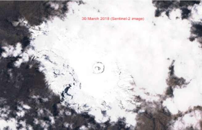
Kilimanjaro's glacier will very probably disappear but so far it does not want to cooperate much with the CO2 hogwash story, because as soon as the atmospheric circulation changes (westerlies, from 270° ±30°, represent only ~5% of hourly means), it snows a lot and Hardy (2018) reported the greatest snowfall on Kilimanjaro glaciers in years (Figure 72).

Figure 72. The Kilimanjaro on March 30, 2018 does not want to cooperate with the anthropic global warming narrative and due to some atmospheric circulation change (westerlies) benefit of the greatest snowfall in years. This anecdotal glacier will keep receding as it has done since its discovery in 1848 and will probably disappear but for other reasons than evil manmade emissions. Source: (Hardy, 2018).

Hogwash I said, in fact not just as we also see deception and scare tactics in action or dumbness and ideology, who knows? Perhaps both!

Before we continue our journey to the Arctic and Antarctica it is worthwhile to spend some time on the way ice-cores are being collected and extracted. In that respect, Jaworowski until his death has been claiming that the way the icecore were interpreted raised a number of questions (Jaworowski et al, 1992a-b; Jaworowski, 1994, 2003, 2007, 2009). It seems that these questions could have been addressed and a common understanding could perhaps have been reached and progress made. But, instead of that and it is sad, leading researchers like Stefan Rahmstorf (2004) in a Munich Re funded paper, had nothing to oppose the perfectly valid reservations issued by Jaworowski (2003) than the ad-hominem attack that he was a self-appointed climate researcher (he knew far more about ice-core than Rahmstorf

will ever213), that his paper was for the laypersons214 and that the journal in which the paper was published belonged to the organization of an American multimillionaire and conspiracy theorist Lyndon LaRouche. What a shame, if I were to dismiss the scientific opinion of Stefan Rahmstorf, and that would be a pleasure doing so, given the weakness of the argumentation he puts forward into his laypersons flyer ordered by a large insurance group, full of affirmations and devoid of proofs, I would not mention first (though I must do it now) that in 1999, he received from an organization representing the legacy of an American multimillionaire industrialist a US$-1m fellowship award from the James S. McDonnell Foundation https://www.jsmf.org/ (isn't there kind of a mental conflict in accepting such a grant when one wants to de-industrialize and decabonize the planet?). One could expect from these system-appointed climate researchers that they would address the problems faced, for example by the ice-core methodologies used and the distortions they induce, which have been courageously and repeatedly underlined by Jarowosky (Jaworowski et al, 1992a-b; Jaworowski, 1994, 2003, 2007, 2009) instead of using ad-hominem attacks, disparagement, ending arguing about the data on a graphic presenting a relationship between cloudiness and cosmic-rays that seems to bring him much frustration. Rahmstorf (2004) rejoices that “Given that the warming is now evident even to laypeople, the trend sceptics are a gradually vanishing breed” forgetting two important things: 1) that neither the UAH data nor the NOAA STT show any warming going further than the natural variability observed throughout the Holocene (appreciate the recourse to the laypersons when supposedly useful whereas he was full of contempt when Jaworowski wrote seemingly for them) and 2) that even though all skeptics might disappear, this is not what will ultimately prove him right and make his scientific legacy destined for a better fate than the dust bin, if he happens to be wrong, what I am sure of. It is unfortunate that Rahmstorf's work did not convince him of how much more the oceans drive the climate, he is a recognized international expert in the domain, than the 0.007% increase of the devil trace gas. Furthermore, Rahmstorf makes as if he would ignore the fact that the reason why the skeptics are disappearing is because of the massive brainwashing and subliminal harassment made by the media and governments, the same that publish and pay him and not because of his overwhelming science. You will notice that I have the highest consideration and respect for Zbigniew Jaworowski215, who had - as a self-appointed multi-disciplinary expert - a very wide knowledge and understanding of all what contributes to making the climate of this planet what it is, whereas I am very wary of narrow views by those appointed to know better than everybody what's good for mankind and each of us.

How funny to read Wikipedia “However, Jaworowski's views are rejected by the scientific community [citation needed]” whereas the “scientific community” is embarrassed enough by Jaworowski's criticisms to have preferred to ignore him and wait for his death, so obviously on July 2020 the citation is more than needed as there are none available. Jaworowski commands the greatest admiration for having written clear and challenging papers until his death in 2011 at 84 years old. Then we can read that “Increases in CO2 and CH4 concentrations in the Vostok core are similar for the last two glacial-interglacial transitions, even though only the most recent transition is located in the brittle zone. Such evidence argues that the atmospheric trace-gas signal is not strongly affected by the presence of the brittle zone.[4]”. The Wikipedia team of authors claim that Jaworowski's concerns would deal with a so-called “brittle zone” and that Jaworowski's arguments could be dismissed on the basis that the consistent GHG records would appear for the Eemian and the Holocene and quote to support their claims .[4] the referenced paper being that of (Raynaud et al., 1994). One will observe that referring to comparisons with the Eemian is highly speculative as, for example, the stratigraphic part of the West Antarctic Ice Sheet Divide Ice CoreCore216 (WAISDIC, 2020) stopped at 31 kyr (the part which is not based on a model, whatever it is, but on the physical counting of layers), therefore far from the Eemian and the brittle zone problems are well acknowledged and documented by Souney et al. (2014), p. 20. Therefore, dismissing Jaworowski's claims by asserting that “the atmospheric trace-gas signal is not strongly affected by the presence of the brittle zone“ is simply a deception and one does not need to go further than the extreme precautions taken by the WAISDIC team (Souney, et al., 2014) to handle the ice cores as of the entire 3,405 meters long of the drill, non-brittle ice was just met from 120 to 520 m and from 1,340 to 2,564 m, the rest having to winter-over at WAIS Divide to give the ice more time to relax before shipment to the analysis facilities at the US National Ice Core Laboratory (NICL)!

To the contrary of what is asserted and to the support of Jaworowski's claims exist several articles, that mention that many problems arise going deeper extracting the ice cores as many physico-chemical phenomenons take place and

213In the 1990s Jaworoswski was already working for the Norwegian Polar Research Institute in Oslo, and for the Japanese National

Institute of Polar Research in Tokyo. In this period he already studied the effects of climatic change on polar regions, and the reliability of glacier studies for estimation of CO2 concentration in the ancient atmosphere. 214What a contempt! Jaworowski's papers are all well written, well documented and always reference relevant work, and they are certainly not only informative for the laypersons, though the term in my writing has certainly no pejorative insinuation, but to everybody, including the scientists of the establishment who should have made the effort to answer his valid questions. 215https://en.wikipedia.org/wiki/Zbigniew_Jaworowski 216https://en.wikipedia.org/wiki/WAIS_Divide and http://waisdivide.unh.edu/about/index.shtml

erase high frequency climate variability, e.g. Pol et al. (2010) state “no new information on MIS 19 climate variability has been revealed, because of a strong smoothing of the deuterium signal. This smoothing, highlighted by a loss of spectral amplitude below a periodicity of ~1600 y, contrasts with the sub-millennial variability preserved for Holocene at comparable resolution and in MIS 19 high resolution calcium data”. In fact, and rightfully pointed out by Jaworowski (1994, 2004), as some water-veins at the grain junctions can be observed under some circumstances, as continuous liquid water network is expected to strongly enhance isotopic diffusion, and as the time period spent by the MIS 19 old ice at temperatures warmer than the critical value of −10 °C which is expected to be a threshold for migration–recrystallization processes could have been too long, all that leads to a loss or distortion of information. This is further obvious when Haan and Raynaud (2002) report dealing just with the last 2,000 years of reconstruction of [CO] “In order to study in detail the pre‐industrial CO level during the last two millennia and its temporal variations, several ice cores from Greenland and Antarctica were analysed. Our Antarctic CO results remain very close to those observed previously for the last 150 years and suggest that carbon monoxide concentration did not change greatly over Antarctica during the last two millennia. Between 1600 and 1800 AD, CO concentrations obtained in the Greenland ice are also very close to those already reported for the 1800–1850 AD period. In contrast, the oldest part of the Greenland CO profile exhibits high CO levels (100–180 ppbv) characterised by a strong variability. This part of the Greenland record likely does not reflect the true atmospheric CO concentrations. We discuss the possible processes which could have altered the atmospheric CO signal either before or after its trapping in the ice. The oxidation of organic material in the oldest part of the investigated Greenland ice appears as the most likely explanation. Because there are strong similarities between the Greenland CO and CO2 concentration profiles for the 1000–1600 AD period, mechanisms involved in both cases could be at least partly the same. Therefore, oxidation of organic materials is a serious candidate for in‐situ CO2 production in the Greenland ice. Due to the fact that the Antarctic ice contains much less impurities and show no peculiar variability in CO concentrations, we are more confident about the atmospheric significance of our Antarctic CO concentration profile”. In the end, these honest authors state the ice-core records might not reflect the true CO concentrations (not the CO2 ones either) that they have more confidence into their Antarctica reconstructions than into the Arctic ones, all that over a very short period of time, 2,000 years. We're not going to show more confidence in their own results than them, and it will obviously be very low. Then the papers from Rubino et al. (2013; 2019) show how much processing and corrections these ice-records require, and indicate that “Additionally, the records have been revised with new, rule-based selection criteria and updated corrections for biases associated with the extraction procedure and the effects of gravity and diffusion in the firn”, confirming what Jaworowski has been saying all along, that there are major side-effects, one of them being the isotopic diffusion due to the increased pressure resulting from the mass of the huge stack of glass accumulated. Finally, Wikipedia writes “ Similarly Hans Oeschger[5] states that "...Some of (Jaworowski's) statements are drastically wrong from the physical point of view", quoting (Oeschger, 1995).

So let's analyze the answer brought by Oeschger and see whether it brings any convincing perspective, the sentences in italic are excerpts from Oeschger's (1995) response paper: • “JAWOROWSKI has induced considerable confusion regarding the reconstruction of ancient atmospheric compositions by the analysis of air occluded in polar ice of known age.” The reader does not learn whether Oeschger thinks Jaworowski's claims are valid of not, he is dubbed a confuser. • “Although we knew since the nineteen fifties that human activities might change the climate of the Earth, it was not until the mid-seventies we realised that mankind was faced with a serious problem. ” Value judgment, unsubstantiated assertion, deception. • “The US-CO2 programme was planned at an ERDA meeting in Miami in the late seventies. At that time we proposed a reconstruction of the CO2 history by measuring the gases trapped in polar ice. This idea was met with great deal of scepticism and we were aware that the changes (sic!) for success were limited because of a wide spectrum of problems, including those which JAWOROWSKI describes in his paper.” So Jaworowski's claims were legitimate and there were not some but a wide range of other problems. The reader will not be entitled to know more, let's continue... • “Some of his statements are drastically wrong from the physical point of view, e.g; the statement that CO2 at 70m depth in the ice begins to change into solid clathrates”. This is the major and in fact sole argument, used by Oeschger to discredit Jaworowski and put forward by Wikipedia, and after verification, Oeschger does not look correct in his affirmation. Let's consider the Phase Diagram P/T, Figure 73, at ~6.4 bars given the ice density of 0.91 and temperatures of the range [-15°C, -40°C] we do not only begin to have hydrates but we are getting straight in the middle of the V-I-H zone. The dark gray region (V-I-H) represents the conditions at which CO2 hydrate is stable together with gaseous CO2 and water ice (below 273.15 K). The pressure is displayed on the left with a logarithmic-scale representation, while temperatures in °C (up) and K (down) are normal scales. Unless one would be unable to find an (X,Y) on a graph, it appears that for ~6.4 bars (~70 meters) and a range

of temperature [-10, -40°C] one falls straight in the dark gray region (V-I-H) where the CO 2 clathrate (H) resides and the more P increases the better sits in the dark gray area. So, unless proven otherwise, Oeschger looks mistaken and Jaworowski correct. Would Oeschger talk of air hydrate, of course they are met much deeper as they are made of 78% N2 and 21% O2 (very different P/T diagram) and therefore reported at respectively 1,092m, 1,099m at Dye-3 Camp Century and 727 m at Byrd Station (Shoji. and Langway, 1987), but Jaworowski mentioned CO2. Furthermore, and unless Jaworowski (1994) would specifically have written it otherwise, Jaworowski (1997) states Fig.2 “Greenhouse gas clathrates begin to form at 80 to 160 m” which gives a pressure range of [~7.3 bars - ~14.5 bars] which is even more in the V-I-H co-existence zone or even beyond into the hydrate stability area. At a mean temperature of -24°C or less, e.g. (Raynaud and Barnola, 1985), one can see that we exit the V-I-H co-existence zone to reach the hydrate stability-only zone at P> ~11.0 bars. So I hardly see how Jaworowski could be wrong and claiming as Oeschger did, on that sole basis, that “his statements are drastically wrong from the physical point of view”.

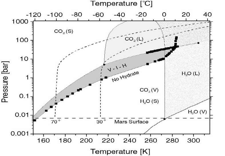
Figure 73. CO2 hydrate phase diagram from Genov (2005), Fig.I.8 p. I-8. The black squares show experimental data (Sloan, 1998). The lines of the CO2 phase boundaries are calculated according to the International thermodynamical tables (1976). The H2O phase boundaries are only “guides to the eye”. The abbreviations are as follows: L - liquid, V - vapor, S - solid, I water ice, H – hydrate.

• “The teams of researchers involved in ice core studies have a high standing within the scientific community.”

What an impressive argument of authority, should such arguments be even taken into account? History of science proves rather the contrary. • “The early increases of the greenhause (sic!) gases are used to initiative (sic!) the models simulating climatic change... The low glacial greenhouse concentrations are an essential boundary condition for climate modelling experiments of the Earth during a glacial period.” So, as the models are initialized with controversial data there is no asking question! • “The papers by JAWOROWSKI, and the one by HEYKE quoted in this paper, are not taken seriously by the science community.” Again a useless and empty argument of authority. They could add, we've been well paid by IPCC for all that deception and Jaworowski was dumb enough to work hard, be right and not make a penny with it! • => then some rantings about the dire consequences of inaction... classical scare mongering tactics, normally used by Greenpeace and the like, but one can also be a reputed professor of Physics at the famous University of Bern and do the same.... • “Based on my experience during decades of involvement in this field, I consider the changes (sic!) as very small that the major findings from greenhouse gas studies on ice core are fundamentally wrong; and I find the publications of JAWOROWSKI not only to be incorrect, but irresponsible” If I understand well: Oeschger has been unable to answer one single question asked by Jaworowski, but he states that he cannot be wrong because

he's been involved for so long that he cannot be mistaken, and finally the cherry on the cake, the argument of morality, Jaworowski is irresponsible because he dares ask questions.

Honestly, I had no opinion before reading the exchange and the response by Oeschger, but if the latter has convinced me of anything, it is to read very carefully what Jaworowski has to say, and to make a head-start on the first and most remarkable statement from him, is “No study has yet demonstrated that the content of greenhouse trace gases in old ice, or even in the interstitial air from recent snow, represents the atmospheric composition ” Jaworowski (1997) and it is simply correct. Shouldn't it have started there?

The validity of current reconstructions of pre-industrial and ancient atmospheres, based on CO2 analyses in polar ice requires that the ice cores fulfill the essential closed system criteria, which basically rests on three fundamental premises Jaworowski et al. (1992a) : “

1. that the age of the gases in the air bubbles is much lower than the age of the ice in which they are entrapped (e.g. Oeschger et al., 1985) ; 2. that 'the entrapment of air in ice is essentially a mechanical process of collection of air samples, which occurs with no differentiation of gas components' Oeschger et al., 1985); and 3. that the original air composition in the gas inclusions is preserved indefinitely”.

Falsifying just one of these assumptions is more than enough to challenge the entire theory of man-made climate change as it rests largely on the reconstructed atmospheres by means of ice cores. None of them will survive an honest analysis and confrontation with the basic facts. The main argument in support of the last two premises is another assumption that no liquid phase occurs in the polar ice at a mean annual temperature of -24°C or less (Berner et al, 1977; Raynaud and Barnola, 1985) but one will observe that this might not be correct because of the existence of a simple thermal gradient as reported, e.g. by Shoji and Langway (1983) “The average bore hole temperature was -20°C from the near the surface to approximately the 900m depth and progressively increased to -12°C at the bottom ”, makes it such that we are far from a required homogeneous -24°C. Jaworowski died at the end of 2011, and it is very unfortunate that this deprived him from first hand confirmation of his reservations, as in July 2012, an exceptional heat wave struck Greenland, creating a melt zone, where summer warmth turned snow and ice into slush and melt ponds of meltwater, and extended to 97 percent of the ice cover (Witze, 2012; Dahl-Jensen et al., 2013). Do not invoke AGW here to explain that it is exceptional and that it did not occur before, because ice cores show that events such as this occur approximately every 150 years on average. The last time a melt this large happened was in 1889. When the meltwater seeps down through cracks in the sheet, it accelerates the melting and, in some areas, allows the ice to slide more easily over the bedrock below, speeding its movement to the sea. During this unusual heat over Greenland in July 2012 melt layers formed at North Greenland Eemian Ice Drilling (NEEM) site as reported by Dahl-Jensen et al. (2013). As the reader can see, the requirement that no liquid phase occurs in the polar ice, so that premises 2) and 3) be reasonable is simply already falsified and much more can be reported.

The first and most obvious evidence that there are a host of physico-chemical processes happening in the ice, is that if the ice was just gently piling up with no physico-chemical transformation happening over the years, the scale of all icecore diagram (CO2 versus depth/age) would be very different, and the age would simply more or less linearly follow the depths (to the variations of the atmospheric supply), whereas it is obvious that the deeper one goes the more condensed the age scale, but with the unfortunate characteristic of neither being a nice log-scale (or else corresponding to a simple physical phenomenon that would let itself easily characterize 217) nor even displaying an homogeneous response across the various sites, e.g. Figure 75 shows well the complete heterogeneity (of the age-scale properties) between the Camp Century core; b, the Byrd core.

In order to help the reader follow a clear logic, the presentation will simply follow the order of the physico-chemical processes leading to the final ice-core in the laboratory. Therefore, the entrapment process will be described first, then the accumulation phase where the ice core progressively is buried deeper under an ever increasing ice load and more numerous ice-layers, like “the P-38 Glacier Girl”, then the drilling process and relaxation that occurs when the sample is extracted, a little bit like when a diver goes back up to the surface.

217It is often assumed that the plastic deformation of ice is generally expressed by a power law in terms of strain rate, έ, and stress σ where A is a constant by: έ = ( σ / A )n (Shoji and Langway, 1983), or by similar expressions but no less empirical, e.g. defined by (Barnes et al., 1971) as έ = A ( sin h α σ )n exp (-Q/RT) where σ is the applied stress, Q an activation energy and A, α and n are suitable constants. The work of (Barnes et al., 1971) deals both with uniaxial compression and basal sheer on rocks (e.g. glacier).

1. When snow is transformed into ice (firnification process) by sedimentation near the surface of an ice sheet, some of the atmospheric air is trapped in the inter-grain spaces which are progressively isolated from the surrounding atmosphere and the resulting material is an “air-tight” bubbly glacial ice, but this progressive transformation does happen over months, years or sometimes decades or more and permits many physicochemical mechanisms to happen (questioning the closed system requirement, i.e. the air trapped must have stayed intact). Therefore, this interaction between the firn and the above atmosphere makes it such that the age of the air in the inclusions may be slightly younger than that of the ice, but one immediately see that this is a process that will show an extreme variance depending on the climatic conditions at the sampling site. This has led to many arbitrary adjustments by those authors wishing to claim that the air is much younger than the ice so that they could also claim that higher CO2 concentrations (inconveniently measured) were related to younger air bubbles than they are in reality. How convenient, isn't it ? If your old reference has too much CO 2, rejuvenate it by claiming that it interacted longer with the surface and here it goes! Doing so, arbitrarily, infringes the 3rd principle enunciated by Jaworowski (2004). Therefore the relative age of the air bubbles with respect to the enclosing ice, i.e. their dating with respect to the age of ice where trapped in leads to interpretations and adjustments. The consolidation of snow to ice necessary to trap the air takes place at a certain depth (the ‘trapping depth’) once the pressure of overlying snow is great enough. Since air can freely diffuse from the overlying atmosphere throughout the upper unconsolidated layer (the ‘firn’), trapped air is younger than the ice surrounding it. But, trapping depth varies with climatic conditions, so the air-ice age difference could vary greatly between a few decades and 6000 years;

2. While the future ice-sample keeps getting older and therefore going deeper, it feels the effect of an increasing pressure. As the phase diagrams for the various gas making up the atmosphere differ significantly, they will also react differently to the pressure increase. In the highly compressed deep ice all air bubbles disappear, as under the influence of pressure the gases change into solid clathrates, which are tiny crystals formed by interaction of gas with water molecules (see Figure 74). The problem is that there always remain some liquid water in ice, which contributes to change the chemical composition the air bubbles trapped between the ice crystals and the more water percolates throughout the cracks during episodic warm summer events, the more disturbances one can fear. In that respect, one should notice that the three main components of the atmosphere have very different basic physico-chemical properties, e.g. carbon dioxide is seventy (70) times more soluble than nitrogen and thirty (30) times more soluble than oxygen. This means that, whenever an air bubble trapped in ice enters in contact with liquid water, not only does the liquid percolating the ice continues to absorb gases, but it does so selectively, favoring carbon dioxide, by a huge margin, over the other common gases in the air bubble and even the coldest Antarctic ice (down to –73°C) contains liquid water as reported by

Mulvaney et al. (1988) studying the existence of liquid veins at grain boundaries state “Calculations show that between 40 and 100% of the sulphuric acid present in this ice was found at the triple-junctions, and would have been liquid at ice-sheet temperatures. This finding, if general, has considerable implications for many of the physical properties of polar ice”. This leads Jaworowski et al. (1992a) to conclude “More than 20 physicochemical processes, mostly related to the presence of liquid water, contribute to the alteration of the original chemical composition of the air inclusions in polar ice”. Of course, every molecule of carbon dioxide that passes into a solution is removed from the air within the air bubble. All these processes necessarily lead to various forms of fractionation, simply because the various gases have different P/T phase diagrams. Fractionation is a direct result of the different reaction of the gases that compose the atmosphere to the increase of pressure as predicted by their different phase diagram P/T. This infringes the first principle listed by Jaworowski (2004) "the entrapment of air (in the ice) is essentially a mechanical process of collection of air samples, which occurs with no fractionation of gas components". At the ice temperature of -15°C dissociation pressure for N2 is about 100 bars, for O2 75 bars, and for CO2 5 bars. “Formation of CO2 clathrates starts in the ice sheets at about 200 meter depth, and that of O2 and N2 at 600 to 1000 meters”. This leads to depletion of CO2 in the gas trapped in the ice sheets. This is why the records of CO2 concentration in the gas inclusions from deep polar ice show the values lower than in the contemporary atmosphere, even for the epochs when the global surface temperature was higher than now.

3. Now, third stage, while drilling and extracting the core, when lifting up the column will let the gas reform from the clathrate and escape the sample throughout the cracks (this is somewhat following similar physicalprocesses to what happens when oil and gas are extracted by fracking). Furthermore various pollutions, contamination and corruption of the T preservation are unavoidable during the drilling, conditioning and transportation processes. While lifting up the ice core the same mechanisms that led to fractionation when the ice accumulated over time are also at play but in a reverse manner as the gases will transit from their hydrate

form to gas again at different P/T (according to the phase diagram) and therefore at different moment and depths thwarting the records in the bubbles. Drilling decompresses cores excavated from deep ice, and contaminates them with the drilling fluid filling the bore-hole. Decompression leads to dense horizontal cracking of cores, by a well known sheeting process. After decompression of the ice cores, the solid clathrates decompose into a gas form, exploding in the process as if they were microscopic grenades. In the bubble-free ice the explosions form a new gas cavities and new cracks as reported by Shoji and Langway (1983) for a 2,037m long ice-core “Deep-ice cores drilled from the Greenland and Antarctic ice sheets undergo volume relaxation due to the expansion of air bubbles with time after core recovery”. These authors also report, and it gives an idea of the stress of the recovered sample, “decreasing rate of hydrostatic pressure of about 5.4bar.min-1 for each core length recovered of approx 1.9m”. Through these cracks, and cracks formed by sheeting, a part of gas escapes first into the drilling liquid which fills the bore-hole, and then at the surface to the atmospheric air. Particular gases, CO2, O2 and N2 trapped in the deep cold ice start to form clathrates, and leave the air bubbles, at different pressures and depth.

Obviously, the assumption that the original air composition in the gas inclusions is preserved indefinitely seems violated all along and confirms the qualms expressed by Jaworowski (2004) “that the original chemical and isotopic composition of atmospheric air trapped in the ice is permanently preserved in the ice sheets and in the decompressed ice cores; this means that the ice should remain a closed system in the ice sheet, in the ice cores during drilling, during decompression from several hundred bar down to one bar, and during transport to laboratory and storage, with no chemical reactions, diffusion through micro-cracks, and gas-liquid-solid phase changes occurring”. As a summary, all these problems arise simply because the ice cores do not fulfill the essential closed system criteria.

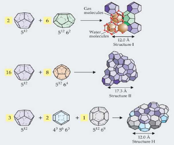
Figure 74. Clathrate hydrates are inclusion compounds in which a hydrogen-bonded water framework—the host lattice—traps “guest” molecules (typically gases) within ice cages. The gas and water don’t chemically bond, but interact through weak van der Waals forces, with each gas molecule—or cluster of molecules in some cases—confined to a single cage. Clathrates typically crystallize into one of the three main structures illustrated here. As an example, structure I is composed of two types of cages: dodecahedra, 20 water molecules arranged to form 12 pentagonal faces (designated 512), and tetrakaidecahedra, 24 water molecules that form 12 pentagonal faces and two hexagonal ones (5 1262). Two 512 cages and six 51262 cages combine to form the unit cell. The pictured structure I illustrates the water framework and trapped gas molecules (from Mao et al., 2007), see also (Brook et al., 2008) and (Everett, 2013).

Let's come back a bit on the lag between the age of the ice and that of the air trapped in it. Berner et al. (1980) considered that atmospheric air can freely circulate in the firn down to the depth at which it finally changes into ice. But at the same time Berner et al. (1980) acknowledge that “Air can circulate in the firn. Measurements on firn samples indicate a loss of CO2 during the sintering process probably due to diffusion of CO2 out of the grains. The transition from firn to ice in Greenland takes place at typical depths of around 70m”, and how that loss is accounted for is not reported. Furthermore, Berner et al. (1980) state “The age of the occluded air is, therefore, younger than that of the ice matrix.

For Greenland, the typical age difference is 200 years. Measurements on samples of young ice from different cold accumulation regions show that the amount of CO2 in the ice lattice is about equal to that in the bubbles”. But the paper is followed by a discussion where Begemann has some questions:

Begemann: “Why is a different CO2 content of the atmosphere not reflected by the CO2 in the ice lattice?“

Oeschger: “We also looked at this question. If Henry's law would hold for the CO 2 fraction in the ice, the varying CO2 content of the atmosphere should be reflected. But the CO2 in the ice lattice may be due to decomposition of organic debris and/or CO2 trapped in refrozen melt layers, ie, phenomena not directly related to the atmospheric CO2 content”.

One should notice that there is a mismatch between the CO2 trapped in the bubbles and that in the ice-lattice. What Bernerd et al. (1980) state is that “Enrichment or depletion of CO2 in the bubbles by exchange with the ice is difficult to estimate”. Furthermore, the relationship between the 70 meters depth and the age, i.e. 200 years is based on a rheological model described by Hammer et al. (1978) and supposed to be better than a 3% error, but one will observe that it does not match with the “P-38 Glacier Girl” burial rate which is perfectly known. Not going to much into the details, in the summer of 1942, the United States started building up troops in the United Kingdom, using Narsarssuak Air Base in Greenland as a stop en route. Among them, bound for the UK, was a flight of six P-38 Lightning fighters and two B-17 Flying Fortress bombers that set out from Greenland on July 15, flying across the North Atlantic to keep their route short but had due to heavy weather in the Denmark straight to return to their base and end up making a forced landing at approximately 150 km west of Angmagssalik near the coast and at less than 200 km away from the future Dye 3 ice core drilling research camp. This is the first time, when the P-38 Echo of Lt. Col. Wilson’s was retrieved in Sept 1989, that one could measure exactly how much ice had accumulated over a given period of time, herein 47 years. The aircraft was buried under 78 meters of snow, firn and ice, which was a lot more than the 12 meters that glaciologists had anticipated and led to reconsider the way the layers were counted and dated (Heinsohn, 1994). The question of why “Glacier Girl” was not more squashed by its long stay under 78 meters of ice and snow is relevant and looking closer at the remains shows that the plexiglass windscreen had exploded and that the aircraft was in fact totally “filled” with snow and ice and where it had not, it had indeed been crushed by the ~5 to 6 bars of pressure (depending on the relative proportions of snow, firn and ice).

So far, we have a rheological model better to 3% accuracy which does not match the observations as the “Glacier Girl” was buried under 78 meters of ice in 47 years (and not 200 years for 70 meters) and two CO2 fractions, i.e. one in the bubbles and one in the lattice, which do not match either. Oeschger finally asserts “The following studies should give information on the origin of the ice lattice fraction: CO 2 measurements on snow and firn combined with chemical analyses, measurements of the isotopic composition of the extracted CO2, laboratory measurements on artificially produced snow and ice samples, etc.”. So, here was the footings on which the AGW story started, not sound as you will agree, but to add a bit to where we stand now, further to the 2012 heat wave Dahl-Jensen et al. (2013) reported that “We reconstructed the Eemian record from folded ice using globally homogeneous parameters known from dated Greenland and Antarctic ice-core records. On the basis of water stable isotopes, NEEM surface temperatures after the onset of the Eemian (126,000 years ago) peaked at 8 ± 4 degrees Celsius above the mean of the past millennium, followed by a gradual cooling that was probably driven by the decreasing summer insolation. . Extensive surface melt occurred at the NEEM site during the Eemian, a phenomenon witnessed when melt layers formed again at NEEM during the exceptional heat of July 2012”.

So far, we know 1) that the previous inter-glacial, the Eemian was much warmer than current conditions and therefore emphasizes that natural variability lead to a far greater variance than observed and that current climate and conditions atop the Arctic are within natural range 2) that melt water percolate throughout the ice sheet and demonstrate that Jaworowski is right in claiming that, necessarily over long periods, say centuries, water drains across the ice sheets and modifies the records, invalidating all the fragile foundations of the AGW theory as no reliable estimates of pre-industrial CO2 atmospheric content can be asserted with reasonable confidence. The depletion in CO2 matches the increase of pressure and reflects a simple fractionation process as the deeper we go into the ice-sheets the more depressed the CO2 content of the core.

Jaworowski (2004) sums everything up “The problem with Siple data (and with other shallow cores) is that the CO2 concentration found in pre-industrial ice from a depth of 68 meters (i.e. above the depth of clathrate formation) was "too high". This ice was deposited in 1890 AD, and the CO 2 concentration was 328 ppmv, not about 290 ppmv, as needed by man-made warming hypothesis. The CO2 atmospheric concentration of about 328 ppmv was measured at Mauna Loa, Hawaii as later as in 1973, i.e. 83 years after the ice was deposited at Siple. An ad hoc assumption, not

supported by any factual evidence, solved the problem: the average age of air was arbitrary decreed to be exactly 83 years younger than the ice in which it was trapped. The "corrected" ice data were then smoothly aligned with the Mauna Loa record (Figure 1 B) , and reproduced in countless publications as a famous "Siple curve". Furthermore, the evidence from direct measurements of CO2 in atmospheric air indicates that the 19th century average concentration was 335 ppmv (Slocum, 1955) and more than 90,000 direct chemical measurements in the atmosphere at 43 Northern Hemisphere stations, between 1812 and 2004 have shown that CO2 varied very significantly [290-440ppm] over that period (Beck, 2007, 2008)218. Finally, and very importantly, a study of stomatal frequency in fossil leaves from Holocene lake deposits in Denmark from Wagner et al. (1999), showing that 9,400 years ago CO2 atmospheric level was 333 ppmv, and 9,600 years ago 348ppmv, falsifies the concept of low and stable CO2 air concentration previous the advent of the industrial revolution. Furthermore, reconstructed CO2 values based on stomatal frequency analysis of fossil Tsuga heterophylla needles show that CO2 values go as high as 400 ppm around 400 AD according to Kouwenberg (2004), Chapter 5, and Kouwenberg et al. (2005). Low and stable CO2 air concentration previous the advent of the industrial revolution is an IPCC deception.

Wagner et al. (1999) state “The inverse relation between atmospheric carbon dioxide concentration and stomatal frequency in tree leaves provides an accurate method for detecting and quantifying century-scale carbon dioxide fluctuations. In contrast to conventional ice core estimates of 270 to 280 parts per million by volume (ppmv), the stomatal frequency signal suggests that early Holocene carbon dioxide concentrations were well above 300 ppmv”. In this important paper, Wagner et al. (1999) report accurate CO2 concentrations and variations for the pre-Boreal Holocene period which were as high as 348 ppmv and state “In the Friesland phase, inferred CO2 concentrations of 265 ± 21 and 260 ± 25 parts per million by volume (ppmv) are followed by a rapid rise to 327 ± 10 ppmv and a more gradual increase to a maximum of 336 ± 8 ppmv in the early part of the Late Preboreal. Then, there is a continuous CO2 decline to a minimum of 301 ± 21 ppmv, followed by a sharp increase to 348 ± 14 ppmv. In the uppermost part of the studied interval, CO2 concentrations stabilize again to values between 333 ± 8 and 347 ± 11 ppmv”.

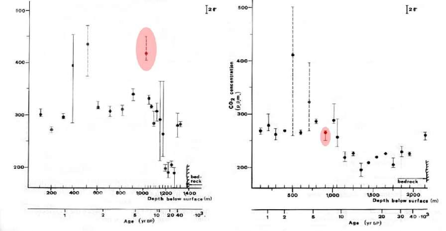
Figure 75. CO2 concentrations in the bubbles and total carbonate content of: a, the Camp Century core; b, the Byrd core. The CO 2 concentrations are presented with the lowest, highest and median values for each depth. The dashed lines indicate depths were drill fluid was observed in the large sample. Maximum CO 2 values of 500 ppm at 500m (~300 years) for the Byrd Core. Modified after: Fig.1 in (Neftel, 1982) with anomalies as pink ellipses ~7,000-year BP added.

218“Meanwhile, more than 90,000 direct measurements of CO2 in the atmosphere, carried out in America, Asia, and Europe between 1812 and 1961, with excellent chemical methods (accuracy better than 3%), were arbitrarily rejected. These measurements had been published in 175 technical papers. For the past three decades, these well-known direct CO2 measurements, recently compiled and analyzed by Ernst-Georg Beck (Beck, 2006, 2007, 2008), were completely ignored by climatologists—and not because they were wrong. Indeed, these measurements were made by several Nobel Prize winners, using the techniques that are standard textbook procedures in chemistry, biochemistry, botany, hygiene, medicine, nutrition, and ecology. The only reason for rejection was that these measurements did not fit the hypothesis of anthropogenic climatic warming. I regard this as perhaps the greatest scientific scandal of our time.” (Jaworowski , 2007)

On the other hand, the ice core data from the Taylor Dome, Antarctica, which are used to reconstruct the IPCC’s official historical record, feature a much more flattish time trend and range, i.e. 285 to 245 ppmv (Indermühle, et al. 1999). This difference strongly imply that ice cores are not a proper matrix for reconstruction of the chemical composition of the ancient atmosphere. Furthermore, Jaworowski (1997) claims that many discrepancies affect the ice cores and that (Oeschger et al., 1985) made an ad hoc attempt to explain some of these anomalies without success and further adds a very specific claim “In about ~6,000-year-old ice from Camp Century, Greenland, the CO2 concentration in air bubbles was 420 ppmv, but it was 270 ppmv in similarly old ice from Byrd, Antarctica”. Though, he does not provide the source of this, it is not difficult to find Fig.1 in (Neftel, 1982) to display exactly that sort of anomaly, though the age is mor e ~7,000-year-old corresponding to 1010 meters at Camp Century, Greenland and 900 meters at Byrd, Antarctica, see for yourself next Figure 75.

So we are left with inaccurate and dubious ice core results as the three fundamental premises are violated because the closed system criteria cannot be met, and which lead the entire AGW edifice to crumble. Pre-industrial CO 2 air concentration of at least 335 ppmv (Slocum, 1955) and pre-Boreal Holocene concentrations of up to 348 ppmv totally invalidate the low and arbitrary cherry picking of Callendar (1938) of 292 ppmv219 which appears more as pathological science (Langmuir, 1989) than anything else. “Callendar was prejudice in selecting from all his data roughly 30%, which showed concentration around 290 ppm, leaving the remaining 70% which showed concentrations over 300 ppm ” (Foscolos, 2010) and he made a disservice to science. This practice of arbitrary selection of data sets matching prerequisites is also prejudicial to science and denounced by Jaworowski (1997) for Neftel at al.; Pearman et al.; Leuenberger and Siegenthaler; Etheridge et al.; Zardini et al.; among others.

Let's give the final point here to Jaworowski (2004), «the basis of most of the IPCC conclusions on anthropogenic causes and on projections of climatic change is the assumption of low level of CO2 in the pre-industrial atmosphere. This assumption, based on glaciological studies, is false. Therefore IPCC projections should not be used for national and global economic planning».

Time now to move on to Antarctica and Arctic. The first will be a rather quick trip as the reader will see that there is not much to say in terms of warming, as it is in fact rather cooling, albeit slowly. Arctic will be more of a challenging place to investigate as it shows some warming and the question will be to try to know what it can be related to. As CO2 is a Well Mixed Gas (WMG), as recalled by Neftel et al. (1982) “Due to atmospheric mixing, the CO2 concentration in the Northern and Southern Hemispheres should not differ by more than a few p.p.m.", one must conclude that any explanation based on GHG warming that would apply only to Arctic and not to Antarctica does not hold.

The West Antarctic Ice Sheet Divide Ice Core, a leading hedge project (WAISDIC, 2020), was completed by the United States Antarctic Program (USAP) and ran under the auspices of the WAIS Divide Ice Core Science Coordination Office (Desert Research Institute and University of New Hampshire) and reports on operations supported by the National Science Foundation under various awards to the Desert Research Institute, Nevada System of Higher Education, and to the University of New Hampshire. They provide a host of information and enable to get a sense of how progress is being made. The site is located at 79°28′03″S 112°05′11″W and is at a linear boundary that separates the region where the ice flows to the Ross Sea, from the region where the ice flows to the Weddell Sea. It is similar to a continental hydrographic divide and was designed so to represent a Southern Hemisphere equivalent to the deep Greenland ice cores. Surprisingly enough, it was asserted that a site in Antarctica was needed because Greenland ice contains enough dust that post-depositional chemical reactions compromise the record of atmospheric carbon dioxide, thus casting a serious doubt on all Arctic records. WAISD drilling was halted 50 meters above the bedrock at a depth of 3405 meters to leave an environmental barrier between the drilling fluid and the pristine basal aqueous environment and intended to provide for a high accuracy of dating of the ice stratigraphy of the most recent 31 kyr based on continuously counting annual layers observed in several indicators, including multi-parameter aerosols (e.g. dust), in the chemical and trace elements, and in records of electrical conductivity, etc. (Sigl, et al. 2016) and led to very accurate dating of key preHolocene events, e.g. “Younger Dryas–Preboreal transition (11.595 ka) and the Bølling–Allerød Warming (14.621 ka)”.

The site was chosen according to a specific criterion. The divide permits to limit the amount of horizontal ice flow drift (<10 meter-year-1 at the basement), thus leading to a better integrity of the ice record (limiting different ice deposition locations for ice at different depths), high annual ice accumulation and thick ice was needed to provide a high time

219To reach the low 19th century CO2 concentration, the cornerstone of his hypothesis, Callendar (1938, 1940, 1949) used a biased selection method. From a set of 26 19th century averages, Callendar rejected 16 that were higher than his assumed low global average, and 2 that were lower, see Fig.1 in (Jaworowski, 2007)

resolution record and led to prefer West Antarctica which has higher ice accumulation rates than East Antarctica, and simple basal topography. The first observation is that the relationship between temperature and accumulation is not as simple as it may appear, and as stated by Fudge et al. (2016a) “the relationship shows considerable variability through time with high correlation and high sensitivity for the 0–8 ka period but no correlation for the 8–15 ka period. This contrasts with a general circulation model simulation which shows homogeneous sensitivities between temperature and accumulation across the entire time period. These results suggest that variations in atmospheric circulation are an important driver of Antarctic accumulation but they are not adequately captured in model simulations. Model-based projections of future Antarctic accumulation, and its impact on sea level, should be treated with caution ”. Here we have a first red flag that clearly identifies that ice stratification and accumulation is certainly not a linear process over time, that it depends on the actual circulation over the site over long periods of time and that just over a 15 kyr timescale, for at the WAISD site, the situation changed from a good to no correlation, whereas the westerlies should have ensured some regularities to the precipitations and accumulation.

When it comes to the identification of the strata, optical stratigraphy or imaging is often performed, but only as long as the contrasts are satisfactory, which was not the case for the entire WAISD ice core. Therefore, a two‐dimensional electrical conductivity stratigraphy was performed for the deepest 40% of the WAIS Divide ice core (1,956 m to 3,405m, 11.5 kyr to 68 kyr) as explained by Fudge et al. (2016b) “The electrical stratigraphy showed clear banding driven primarily by annual variations. Centimeter‐scale pinched layers and other irregularities were concentrated between 2700 m and 2900 m (27 ka to 33 ka); below 2900 m, decreasing amplitude of conductance variations likely due to diffusion prevented confident interpretation of both annual and irregular layering”.

So, beyond 33 kyr and using the best techniques, the records get fuzzy displaying irregular layering which arises from variations in the deformation of ice due to strain and sheer even in a limited flow conformation due to the divide between the Ross Sea and the Weddell Sea and Fudge et al. (2016b) report “below 2900 m, decreasing amplitude of conductance variations likely due to diffusion prevented confident interpretation of both annual and irregular layering. The effective diffusivity at −30°C is 2.2 × 10−8 m2 yr−1, approximately 5 times greater than for self‐diffusion of water molecules, implying diffusion at grain boundaries... the irregular layering likely arises from variations in the deformation of ice”. So, here one starts seeing the processes described by (Jaworowski, 1997), stress, cracks, strain, sheer, diffusion, which for the WAISD ice core represented 1,780 m (0 to 120m, 520 to 1,340m and 2,565 to 3,405m) over the entire 3,405 m, i.e. nearly 53% of the entire total of the ice core and I will add gas fractionation which is not visible but inevitable and intimately linked to the increase of pressure as we talk at the bottom of the drill of kind of three hundreds (300) bars, and finally decompression and selective degassing when the sample is extracted.

Despite the fact that glacial stratigraphy is always complex as it has just been noted, if only because it provides intertwined levels, with deposition processes leading to layers displaying unconformity and nonconformity due to climatic hazards, etc. the simple ice flow and the annual numbering of the ice strata resulted at WAISD in the first record of ice stratigraphy and accumulation rate back to the Antarctic Isotope Maximum 4 (AIM) warm event that is independent of an assumed relationship to water stable isotopes. Alas, the ice accumulation rate did not consistently correlate with water isotopes, particularly at times of abrupt climate change in the Northern Hemisphere (Fudge et al., 2016a, 2016b). “This calls into question the common practice of using water isotopes as a surrogate for the ice accumulation rate” (West Antarctic Ice Sheet (WAIS) Divide Project Members, 2013; Buizert et al., 2015).

Be it for previous studies, e.g. (Neftel, 1982; Neftel et al., 1988) where the bedrock was met before 60 kyr, be it at Camp Century (Arctic) or Byrd (Antarctic), the WAISDIC results confirm that even 20 years later the first studies and with significant instrumentation progress, the bedrock remains where it is and that 31 kyr of real chrono-stratigraphy is a great achievement and 68 kyr is the limit which is reached only at the cost of widely increased uncertainties. The chronology for the deeper part of the core (67.8–31.2 kyr BP), was reportedly based on stratigraphic matching to annual-layer-counted Greenland ice cores using globally well-mixed atmospheric methane. Buizert et al. (2015) report “We calculate the WD gas age–ice age difference (Δage) using a combination of firn densification modeling, ice-flow modeling, and a data set of δ15N-N2, a proxy for past firn column thickness. The largest Δage at WD occurs during the Last Glacial Maximum, and is 525 ± 120 years”.

One will immediately notice that the techniques used have drastically changed and that using a combination of models and proxies for the firn column thickness, a Δage is then assessed and Buizert et al. (2015) add “Internally consistent solutions can be found only when assuming little to no influence of impurity content on densification rates, contrary to a recently proposed hypothesis. We synchronize the WD chronology to a linearly scaled version of the layer-counted Greenland Ice Core Chronology (GICC05), which brings the age of Dansgaard–Oeschger (DO) events into agreement with

the U/Th absolutely dated Hulu Cave speleothem record”. That's a lot of geo-engineering to make things match and show somehow some coherence down to the 68 kyr limit. In any case, the site does not provide information on the status of WAIS during MIS-5e because basal melting would have melted any ice from that time.

Therefore, one will wonder how much 800 kyr reconstructions can be trusted and with which confidence and reliability the results should be considered as it takes us more than 10 times further back than what appeared already as a technological prowess with the wherewithals of a unique and recent project (2006-2013), such surprisingly distant reconstructions are provided by e.g. (Jouzel et al. 2007; Bereiter et al., 2015) and one must notice that they do not rest on any real stratigraphic counting, just on modeling (firn densification, water isotopes, etc.). The European Project for Ice Coring in Antarctica (EPICA) has provided two deep ice cores in East Antarctica and the drilling at Dome C, was stopped at a depth of 3260 m, about 15 m above the bedrock. As stated by Jouzel et al. (2007) “A preliminary lowresolution δD220 record was previously obtained from the surface down to 3139 m with an estimated age at this depth of 740,000 years before the present (740 ky B.P.), corresponding to marine isotope stage (MIS) 18.2 (1)... We completed the deuterium measurements, δDice, at detailed resolution from the surface down to 3259.7 m. This new data set benefits from a more accurate dating and temperature calibration of isotopic changes based on a series of recent simulations performed with an up-todate isotopic model”.

One will notice that it is not mentioned any longer the existence of any stratigraphic ice age records that would serve as a validating reference to the far extending δDice, but of simulations based on ad-hoc isotopic model. The accuracy envisaged by the authors, and one will hardly understand how it can remain constant and stable over the entire 740 kyr given what was seen over the 15 kyr period at the WAISD site with accurate records, is mentioned as “ EDC3 has a precision of ±5 ky on absolute ages and of ±20% for the duration of event”.

Furthermore, one will also notice that the only validation of the entire results reported depends on another piece of software, i.e. a GCM as stated by Jouzel et al. (2007) “Results derived from a series of experiments performed with the European Centre/Hamburg Model General Circulation Model implemented with water isotopes (9) for different climate stages (SOM text) allowed us to assess the validity of the conventional interpretation of ice core isotope profiles (δD or δ18O) from inland Antarctica, in terms of surface temperature shifts”. So, we have simulations performed according to an ad-hoc isotopic model which are validated by another piece of obscure software which is a general circulation model, and this is how the temperatures are known, all that is truly impressive but one remains cautious, aren't you ?

One thing for sure, with Jouzel et al. (2007) one is more into the response of a modeling system than into the stratigraphic counting of the ice layers, which even when done with the greatest care starting from ad-hoc drilling procedures, e.g. (Shturmakov, 2007)221 and (Souney et al., 2014) show that beyond tens of kyr problems start piling up, not even considering all reservations brought up by (Jaworowski et al, 1992a-b; Jaworowski, 1994, 2003, 2007, 2009).

As one can always find positive information, and provided that the results can be trusted notwithstanding all observations made, one will notice that the climate changes mentioned over the 740 kyr record show a natural variability which far exceed the current changes observed throughout the last two millenniums and Jouzel et al. (2007) state “We inferred that the change in surface temperature (ΔTs) range, based on 100-year mean values, was ~15°C over the past 800 ky, from -10.3°C for the coldest 100-year interval of MIS 2 to +4.5°C for the warmest of MIS 5.5 ” which means huge natural amplitudes and a Δts of up to 15°C! Of course without any man-made emission...

At that time, i.e. 2007, the authors were of the opinion that “peak temperatures in the warm interglacials of the later part of the record (MIS 5.5, 7.5, 9.3, and 11.3) were 2° to 4.5°C higher than the last millennium” and considered that “the interplay between obliquity and precession accounts for the variable intensity of interglacial periods in ice core records”. It seems that some CO2 mind-blurring has happened in the meantime and they are looking now with the IPCCC for another explanation were sort of +1.6 W/m2 (maximum but probably much less in the order of +1.0 W/m2) of CO2 IR absorption (for a doubling) would produce stronger effects than just the variation of the obliquity (notwithstanding all other factors) that they reported by then as representing ten times more at +14 W/m 2, Jouzel et al. (2007) “With respect to the strong linear relationship between δD and obliquity, the link may be local insolation changes, which at 75°S vary by ~8% up to 14 W/m2 . ”

220D stands of course for Deuterium. 221e.g. the drill fluid is a mixture of HCFC 141b (densifier) and Isopar K (base solvent).

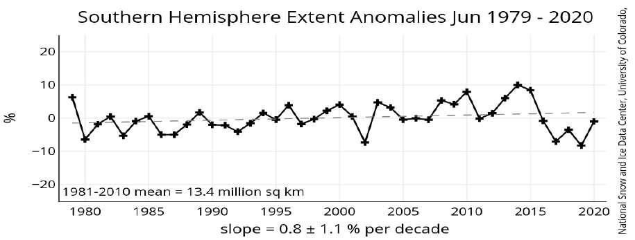
Figure 76. Antarctica monthly sea ice extent anomaly as per https://nsidc.org/data/seaice_index shows a +0.8 ± 1.1% increase per decade. Methodology described at https://nsidc.org/sites/nsidc.org/files/G02135-V3.0_0.pdf

So now the good news, which is that whatever the IPCC speculations and the arguing about the next Armageddon if all the emissions are not cut drastically, the Antarctica has kept growing (Wang et al., 2019), yes growing albeit at a small pace, i.e. +0.8 ± 1.1% per decade, and the graph Figure 76 (National Snow & Ice Data Center - University of Colorado, Boulder) is quite clear.

And as a picture is worth a thousand words, let's see the geographical extent of the sea ice and compare it to its median ice edge (1981-2010):

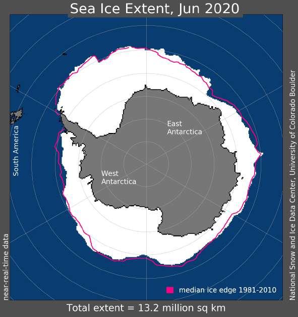
Figure 77. The monthly Sea Ice Index provides a quick look at Antarctic-wide changes in sea ice. It is a source for consistently processed ice extent and concentration images and data values since 1979. Monthly images show sea ice extent with an outline of the 30-year (1981-2010) median extent for that month (magenta line), as per https://nsidc.org/data/seaice_index. Source: National Snow & Ice Data Center - University of Colorado, Boulder.

Finally, the following graphic depicts the temperature in Antarctic with the Ln(CO 2) and shows that despite the massive increase in [CO2] there is simply no temperature response for the simple reason, that the climate has a very low sensitivity to CO2 as we have amply demonstrated up to now.

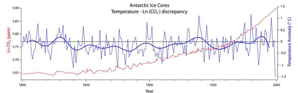
Figure 78. CO2 curve (red) from Antarctic Ice Cores Revised 800 kyr CO 2 Data (to 2001). Source: NOAA, contributed by Bereiter et al., (2015); and from NOAA annual mean CO2 data (2002–2017). Due to the logarithmic effect of CO2 on temperatures, the comparison is more appropriately done with the Ln(CO 2). Temperature curve (blue) for the past 200 years from 5 high resolution Antarctic ice cores. Source: Schneider et al. (2006). No temperature change is observed in response to the massive increase in CO2, over the period 1800-2000 (despite the conclusion from Schneider et al. (2006), who by cherrypicking the data, says slightly otherwise). Source: Javier (2018b).

Surprisingly, Antarctica shows absolutely no warming for the past 200 years as displayed on Figures 76, 77 and 78. The only place where one can measure both past temperatures and past CO2 levels with some confidence for 31 kyr shows no temperature response to the huge increase in CO2 over the last two centuries and at least for the last 7 decades as evidenced by a thorough analysis by Singh and Polvani (2020). This evidence supports that CO2 has very little effect over Antarctic temperatures, if any, and it cannot be responsible for the observed correlation over the past 800,000 years, and again appears just as a lagging proxy on the temperature. “It also raises doubts over the proposed role of CO 2 over glacial terminations and during Modern Global Warming (MGW)” (Javier, 2018b).

Measurements are directly available and can be checked for a host of different stations. A very limited excerpt of some stations is listed hereafter and show no warming over the period 1950-2020 :

Station Data: Halley (75.45S, 26.217W): https://data.giss.nasa.gov/cgi-bin/gistemp/stdata_show_v4.cgi?id=AYM00089022&ds=14&dt=1 Station Data: Mawson (67.6S, 62.8670E): https://data.giss.nasa.gov/cgi-bin/gistemp/stdata_show_v4.cgi?id=AYM00089564&ds=14&dt=1 Station Data: Vernadsky (65.25S, 64.267W): https://data.giss.nasa.gov/cgi-bin/gistemp/stdata_show_v4.cgi?id=AYM00089063&ds=14&dt=1 Station Data: Dumont D'Urville (66.667S, 140.0170E): https://data.giss.nasa.gov/cgi-bin/gistemp/stdata_show_v4.cgi?id=AYM00089642&ds=14&dt=1 Station Data: Jan Mayen (70.9331N, 8.6667W): https://data.giss.nasa.gov/cgi-bin/gistemp/stdata_show_v4.cgi?id=NOE00105477&ds=14&dt=1 Station Data: Bjoernoeya (74.5167N, 19.0167E): https://data.giss.nasa.gov/cgi-bin/gistemp/stdata_show_v4.cgi?id=NO000099710&ds=14&dt=1 Station Data: Nikolskoye Beringa Ostrov (55.2000N, 165.9800E): https://data.giss.nasa.gov/cgi-bin/gistemp/stdata_show_v4.cgi?id=RSM00032618&ds=14&dt=1 Station Data: Barrow Post Rogers Ap (71.2833N, 156.7814W): https://data.giss.nasa.gov/cgi-bin/gistemp/stdata_show_v4.cgi?id=USW00027502&ds=14&dt=1

Complete access is provided here, selecting stations at will on the sensitive globe display: https://data.giss.nasa.gov/gistemp/station_data_v4_globe/

It has long been considered by most authors that the change of CO2 levels between glacial and interglacial periods, of only 70–90ppmv, is too small to drive the glacial cycle, and even if Shakun et al. (2012) state that “Our global temperature stack and transient modelling point to CO2 as a key mechanism of global warming during the last deglaciation” not only does their excellent paper totally invalidates that assertion but also provides for a clear sequence of event of how a deglaciation happens and of how little the CO 2 plays a role. We now have seen all the required concepts to describe the full scenario of how the Earth exists a glacial era, let's see how that works.

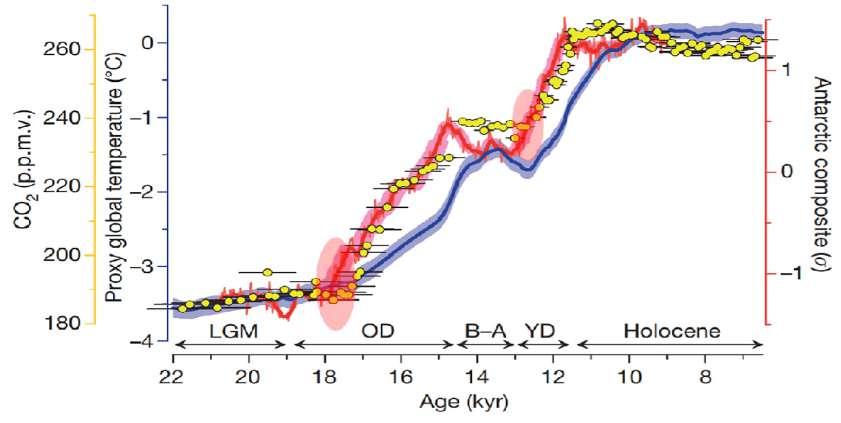
Figure 79. Temperature(s) T and CO2 concentration: The graph displays the global proxy temperature stack (blue) TG as deviations from the early Holocene (11.5–6.5 kyr ago) mean, an Antarctic ice-core composite temperature record (red) T A, and atmospheric CO2 concentration (EPICA Dome C ice core). The pink ellipses show clearly where TA starts rising before CO2 which keeps lagging all along except for the degassing hysteresis oceanic effect when T stabilizes (between -15 and -13kyr). The Holocene, Younger Dryas (YD), Bølling–Allerød (B–A), Oldest Dryas (OD) and Last Glacial Maximum (LGM) intervals are indicated. Modified after: Shakun et al. (2012).

1) As with seen Figure 36, the sinusoidal change of obliquity, with the help of precession, leads to an increase in insolation at 65N at around -19 kyr. This does not succeed to produce the initial trigger the exit of the glacial era each time, i.e. every 41 kyr, as the Earth as gotten cooler and cooler, and since the previous inter-stadial, i.e. the Eemian, two unsuccessful attempts failed until the Holocene turned out to be the right one. It is remarkable that it was not until Roe (2006) that it was recognized that during the alternation of deglaciations and glaciations, the insolations at 65°N from Milankovitch's calculations are not correlated with the ice volume

V(t), deduced from the sea level found by various geological markers, but with the time rate of change of global ice volume, i.e. the derivative dV/dt of this volume with respect to time! It is however obvious that temperature determines the melting of the ice dV/dt, and not its volume V(t), and thus that there exists a relationship of the kind: dV /dt= a (T(t) - T0) b. By doing so, Roe (2006) reports that “the available records support a direct, zero-lag, antiphased relationship between the rate of change of global ice volume and summertime insolation in the northern high latitudes. Furthermore, variations in atmospheric CO2 appear to lag the rate of change of global ice volume. This implies only a secondary role for CO 2 – variations in which produce a weaker radiative forcing than the orbitally-induced changes in summertime insolation – in driving changes in global ice volume”. Then, and this is very important, Shakun et al. (2012) state “Substantial temperature change at all latitudes, as well as a net global warming of about 0.3°C, precedes the initial increase in CO2 concentration at 17.5 kyr ago, suggesting that CO2 did not initiate deglacial warming”. Not only did CO2 not initiate the deglacial warming, but contrary to what Shakun et al. (2012) try to demonstrate by using monte-carlo simulations, CO2 did not play any role at all, just lagged the temperature and especially those in Antarctica (as they concede anyway) where the degassing of the southern oceans produced the increase in the gas of life, this being very well visible on Figures 71 and 79, e.g. (Martínez-Botí et al. 2015). Each of the pink ellipses show that the Antarctica temperature broke out of a consolidation phase first (at 12.5 and 17.8 kyr) and second CO2 followed, and that when the temperature stabilized horizontally, CO2 slightly overshot due to the hysteresis effect of the warmer ocean which kept degassing, given the long residency time of the AMOC, and finally started to subside.

2) This warming of the Northern mid to high latitudes, due to the orbital trigger, were the first to warm after the LGM leads to the observed retreat of Northern Hemisphere ice sheets and the increase in sea level commencing 19 kyr ago, with an increase of freshwater that produces a weakening of the AMOC. In response to 1.0-Sv freshwater input, the THC switches off rapidly in all model simulations. A large cooling occurs over the North Atlantic. The annual mean Atlantic ITCZ moves into the Southern Hemisphere (Stouffer et al., 2006) ;

3) At that point there occurs a a pronounced inter-hemispheric seesaw event around -13.5 kyr, as seen in the Pa/Th (protactinium/thorium ratio) record and Shakun et al. (2012) state “We find that ΔT decreases during

the Oldest Dryas and Younger Dryas intervals, when the Pa/Th record suggests that the AMOC is weak and heat transfer between the hemispheres is reduced, and that ΔT increases during the LGM, the Bølling–Allerød and the Holocene, when the AMOC is stronger and transports heat from the south to the north”. There results a cooling of Arctic between 13.8 kyr to -12.5 kyr, but the tropical and Southern Hemisphere warming seem to completely offset northern extra-tropical cooling. A near-synchronous seesaw response is seen from warming of the mid southern latitudes to the cooling of the high northern latitudes, and strong Antarctic warming is observed and the increase in CO2 concentration obviously lags the temperature and the AMOC change, as it is the very change in the AMOC circulation which leads to an increase in the degassing of the southern oceans. There exists a correlation between times of minima in the AMOC and maxima in CO2 release, for the simple reason that to a minimal northern AMOC corresponds warmer southern oceans and more degassing. Anderson et al. (2009) observe “In the record with the greatest temporal resolution, we find evidence for two intervals of enhanced upwelling concurrent with the two intervals of rising atmospheric CO2 during deglaciation. These results directly link increased ventilation of deep water to the deglacial rise in atmospheric CO2”.

4) The entire Bølling-Allerød period -12.7 to -14.7 kyr was a climatically unstable period in the northern high latitudes and this instability is linked to alternating modes of the Arctic sea ice cover between periods with and without perennial sea ice cover. Then the AMOC resumes around -12.5 kyr and the northern hemisphere and the Arctic warm again to reach a high level at the beginning of the Holocene, at the end of the Younger Dryas, at -11.7 kyr, but the Holocene Climatic Optimum will only be reached slightly later, during the Boreal at around -9.7 kyr (Figure 35).

As was clearly explained above, CO2 has been accompanying the events, nothing more and acted as a ex-post thermometer just recording the increase in temperatures through the simple effect of Henry's law and the obsessional focus on it to try to explain a much more complex sequence of event is surprising. Thus the final statement by Shakun et al. (2012) “Our global temperature stack and transient modelling point to CO2 as a key mechanism of global warming during the last deglaciation” seems to simply go against all evidences brought by the paper and contradicts the very title of the article.

Over the last 200 years CO2 levels have increased by 78 ppm (335 ppmv before the industrial age and 413 ppmv as of July 2020), an increase comparable to that of a glacial termination in terms of additional CO2. But, Antarctica shows absolutely no warming for the past 200 years and this evidence supports that CO2 has very little effect over Antarctic temperatures, if any, confirms the very low atmospheric sensitivity to CO2 and it cannot be responsible neither for the termination of the glacial cycle, as Shakun et al. (2012) have rightfully acknowledged, nor of the modern warming which started at the end of LIA. As far as very recent times are concerned, since 1958, Curry (2018) reports “ Temperature reconstructions for Antarctic show little change in East Antarctic surface air temperatures, but warming since 1958 over West Antarctic and the Antarctic Peninsula (Nicolas and Bromwich, 2014). Since the late 1990s, the Antarctic Peninsula has cooled, decadal temperature changes for West Antarctic and the Antarctic Peninsula are within the large natural climate variability (Turner et al., 2016; Smith and Polvani, 2017)” (Curry, 2018). In fact, a recent paper rather shows that East Antarctica has been rapidly cooling in recent decades, with magnitudes reaching -0.7°C to -2.0°C per decade since the mid-1980s (Obryk et al., 2020). How unfortunate, it seems that the whimsical climate does what it wants and does not stick to AGW climate-illusionists injunctions.

It does not look like the house is on fire, doesn't it?

Actually, the Arctic displays some kind of unusual response since the mid of the 1980s, though it is not the first time as the north polar cap shows a much greater sensitivity to weather and climate changes than the other pole; in that respect the free e-book from Longhurst (2015) addresses very well this topic through its section 8.1-8.4 and its reading is highly recommended. Let's start with a question: do you remember the settlement of the Vikings on the “Green Land” with Erik the Red in 985, who was the first permanent European settler, during the Medieval Warm Period?. The Icelanders established two colonies just after sailing past Cape Farewell, a headland on the southern shore of Egger Island, Nunap Isua Archipelago at the southern extremity of Greenland, one on the extreme southwest coast known as the the Eastern Settlement222 or Eystribyggð (which was in fact just close to the extreme South), now Qaqortoq, and the Western Settlement, close to present-day Nuuk. The Norse settled at the head of long fjords and grew up to 4,000 inhabitants, with more than 500 groups of ruins of Norse farms known and a diet which consisted initially of 80% of agricultural products and 20% marine food (Arneborg et al., 1999).

222https://en.wikipedia.org/wiki/Eastern_Settlement

This says a lot about the climate as it must have enabled at that time the growth of enough hay meadows during summertime to feed livestock, and undoubtedly, around year 1000, Greenland was warmer and nearly devoid of ice a significant part of the year, at least in most of the surroundings of southern fjords where the Eastern Settlement was. From the 14th century on the Greenland Norsemen had 50–80% of their diet from the sea and had undergone an adaptation process to climate change, but as stated by Dugmore et al. (2010) it is estimated “that the Norse had achieved a locally successful adaptation to new Greenlandic resources but that their very success may have reduced the long term resilience of the small community when confronted by a conjuncture of culture contact, climate change, and new patterns of international trade”. In any case, a wedding solemnized in 1408, is the last recorded contact with the colony, placing it about 50–100 years later than the end of the more northern Western Settlement, the Norse are considered to have deserted around 1,450 whereas the the Thule Inuit survived through the period of Norse extinction. The more than 400 years of settlement ended by an abrupt collapse, due as always to cooling conditions and certainly not warming, as the entire history of mankind tells us, and that we should remember if History is any guide. Today, farming is still the main occupation in Qassiarsuk and the local sheep farmers in the area cultivate the same fields and graze their animals on the same hillsides that the Norsemen used more than a thousand years ago, and they certainly welcome the milder climate than that of the LIA.

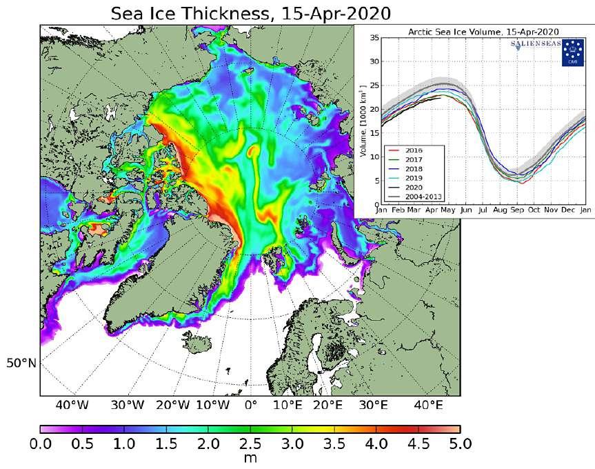
Figure 80. The Sea Ice Thickness and extent provides a quick look at Arctic-wide changes in sea ice, here for April 15, 2020, somewhere around its maximum yearly extension as displayed in the superimposed sinusoid. Source: from the Danish Meteorological Institute (DMI), as per http://ocean.dmi.dk/arctic/icethickness/images/.

As reminded by Longhurst (2015) “The entire record - in which 20th century temperature are rather similar to those of the Mediaeval Warm Period - is marked by multi-decadal oscillations over 2-3°C so that, consequently, the observed recent changes are not unusual either in scale or duration: the ice-core record of temperature thus confirms historical evidence (Kobashi et al., 2010)” and Kobashi et al. (2011) assert “Therefore, we conclude that the current decadal mean temperature in Greenland has not exceeded the envelope of natural variability over the past 4000 years”. Furthermore, as explained by Longhurst (2015) “But the present glacier retreat is not a uniform phenomenon, as it is usually portrayed. On Bylot Island, across Baffin Bay from the Greenland coast at about 73°N, a party of Canadian geologists in summer 2009 found that almost all of the glaciers were at their terminal moraines, implying a regional lack of glacier retreat”. Checking the details of this information in Wielens et al. (2009) p. 25, one will be surprised to read “ The glaciers on Bylot Island are striking. Virtually all are at their end moraines, the ground-up rocks deposited farthest out by the snout of the glacier, and crevasses are present only over 'steps' in the underlying bedrock”. Obtaining striking

images of glaciers calving massive discharges of ice in the sea is better for publishing a successful paper in the newspress, and a well known site to obtain such pictures is the Ilulissat glacier (also known as Jakobshavn Glacier 223) which calves abundant icebergs into Disko Bay and did so throughout the XX th century, the Titanic iceberg is thought to have come from it in 1912. Thus the behavior of the glacier is very differential and the AGW meme puts the emphasis on the glaciers that recede, as the Wikipedia paper does, forgetting all the others. But as will be next explained, the behavior of the regional glaciers and of the Arctic more generally coincides with the influence of Atlantic waters through the various oscillations known as the AMO e.g. (Chylek et al., 2011) or e.g. a negative phase of the NAO, i.e. anti-correlation of (r=–0.84 to–0.93) with the Greenland temperatures (Chylek et al., 2004), etc. and not with any radiative imbalance.

Having reminded of the natural variability through historical and regional records, which is always a good start to make an informed reasoning, clearly, since the mid-1980s, the mass balance has switched in Arctic, in fact the Decadal Mass Balance (DMB) of the entire Greenland ice sheet tilted from a mass gain of +47 ± 21 Gt/y in 1972–1980 to a loss of -51± 17 Gt/y in 1980–1990 but showed that the ice sheet as a whole was near balance over the time period 1972–1990 (Mouginot, et al., 2018). Of course, to make such an assertion, a lot of modeling has to take place as the only way to access with some reliability the evolution of the Total Mass Balance (TMB) is through the Mass Budget Method (MBM) that provides information about the physical processes controlling the mass loss made 1) through the Surface Mass Balance (SMB) processes made of accumulation minus runoff and other forms of ablation and 2) glacier dynamics (basal ice mass flux into the ocean). Knowing precisely the TMB requires to assess the precise glacier fluxes into the ocean and reconstruction of SMB over the ice sheet. The major change leading to a negative DMB is an increase of the basal ice discharge under the influence of tidewater glaciers responding to the Atlantic Multidecadal Oscillation 224 (AMO). The oceanic influence is always from where the triggers come and the action of the AMO in Arctic is mirrored somehow by what is also happening in Western Antarctica where the tips of glaciers under the influence of oceanic tides also show some increased discharge (whereas TMB is positive). As was said, the computation of TMB requires a lot of modeling to determine on the one hand the accumulation of snowfall (from regional atmospheric climate models) and on the other the mass loss based on Digital Elevation Model DEMs (using among other sources of information radar surveys and airborne laser altimetry) which yields a time series of glacier thickness to calculate glacier fluxes with precision in Greenland since 1972, i.e. the start of the Landsat historical archive. Provided that one trusts the models, the discharge has increased since the 1980s and especially the mid-1980s, but this comes as no surprise as when one looks at the Arctic ice volume in the upper corner of Figure 80, one can visibly see that 2020 is at the bottom of the short-term variability, but 2018 just 2 years ago was within the gray envelope representing the mean for the decade 2004-2013.

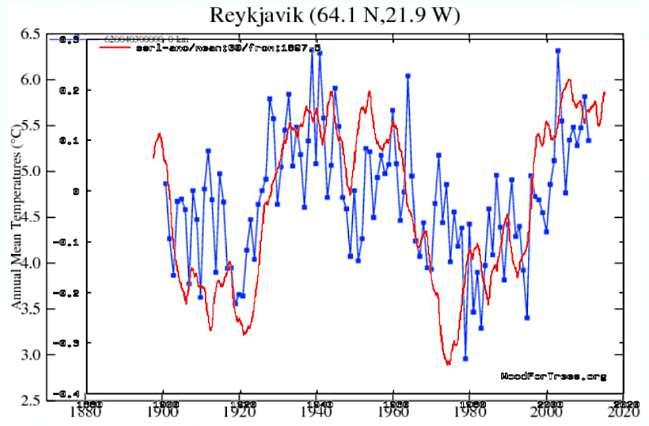
Figure 81. GISS Surface Temperature Analysis (in Blue), Station Data: Reykjavik (64.1 N, 21.9 W) 225 Iceland and Atlantic Multidecadal Oscillation (AMO) (in Red) “ESRL AMO index226” superimposed. Eastern Arctic temperatures closely track the Atlantic Multidecadal Oscillation, and show no correlation with atmospheric CO2. Source: https://realclimatescience.com/arcticsea-ice-unchanged-from-60-years-ago/.

223https://en.wikipedia.org/wiki/Jakobshavn_Glacier 224https://en.wikipedia.org/wiki/Atlantic_multidecadal_oscillation is a climate cycle that affects the sea surface temperature (SST) of the North Atlantic Ocean . 225https://data.giss.nasa.gov/cgi-bin/gistemp/show_station.cgi?id=620040300000&dt=1&ds=1 Directly from NASA web page where one can get any data for any station wished.

226https://woodfortrees.org/plot/esrl-amo/mean:60/from:1897.5

Let's remind first that CO2 is a Well Mixed gas (WMGG), e.g. “Due to atmospheric mixing, the CO2 concentration in the Northern and Southern Hemispheres should not differ by more than a few p.p.m." (Neftel et al., 1982) and “Air is well mixed with only minor variation in CO2 content with latitude” (Latour, 2014). Thus, any explanation based on GHG warming applying only to Arctic and not to Antarctica does not hold, the limited warming in Arctic is not the consequence of the observed increase of CO2. This is anyway what was stated by Chylek et al. (2006) in the clearest way “To summarize, we find no direct evidence to support the claims that the Greenland ice sheet is melting due to increased temperature caused by increased atmospheric concentration of carbon dioxide”. As was presented while addressing the oscillations and the oceanic currents and the scenario that enabled the Earth to exit the last glacial era to enter the milder Holocene, Arctic has proved very sensitive to the influence of the THC and of the Atlantic Multidecadal Oscillation (AMO) in particular, to which it responds with the regularity of a metronome.

From the previous Figure 81, one can see multiple important patterns, first Eastern Arctic temperatures and temperatures in Iceland show no alarming sign of warming (not above the 1930-1940 period representing a comparable very short term variability, see also Mikkelsen et al. (2018) Fig.2 p. 6), and second and more importantly, they closely follow the AMO with great regularity. Let's remind ourselves again that the AMO is an oscillation that affects the sea surface temperature (SST) of the North Atlantic Ocean on multidecadal timescales and ocean circulation drives the phase changes of the AMO by controlling ocean heat content and exchange. McCarthy et al. (2015) remind that “Positive (negative) phases of the AMO coincide with warmer (colder) North Atlantic sea surface temperatures. The AMO is linked with decadal climate fluctuations, such as Indian and Sahel rainfall, European summer precipitation, Atlantic hurricanes and variations in global temperatures”. Furthermore, ocean circulation appears to result from atmospheric triggers, refer to the NAO described before, through circulation changes between the sub-tropical and subpolar gyres, i.e. the inter-gyre region.

Studying the AMO variability over some decades, Ting et al. (2008) observe “However, the earlier warming trend in the 1930s and the cooling trend in the 1970s were connected mainly to internal variability”. They also report that beyond the Atlantic surrounding which is under direct influence of the AMO, its effects are felt much further and the largest impact is over the Sahel region, where the warming trend of the AMO is associated with increased precipitation and reversely the epoch of the Sahel drought of the 1970s and 1980s is associated with a cooling trend in the AMO and opposite for the Yucatan peninsula (Knudsen et al., 2011), Fig.2. All that reminds us that the climate is first and foremost made of precipitations and natural variations (Koutsoyiannis, 2008), that it has always been the case and not of a minuscule increase of CO2 concentration.

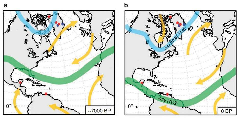
Figure 82. a) ~-7,000 years with significantly higher NH summer insolation than today, whereas it was lower in the SH (opposite in winter) led to a shift of the ITCZ, located north of its present position, with the PF also displaced well to the north in the North Atlantic sector. These conditions may be representative for the average conditions between -6,000 and -8,000. b) Modern atmospheric systems of the North Atlantic region (may also represent average conditions for the period 0–3,000 years BP, where an overall ‘neo-glacial’ regime with more frequent meridional atmospheric circulation patterns. PF, atmospheric Polar Front; ITCZ, Inter-Tropical Convergence Zone. The yellow arrows indicate the dominant wind directions and explain why it rained 7,000 years in the Green Sahara, whereas dry Trade winds prevail today. After Ting et al. (2008).

Ting et al. (2008) have shown, based on spectral analyses of high-resolution climate proxy records from the region bounding the North Atlantic, that distinct ~55 to 70-year oscillations characterized the North Atlantic oceanatmosphere variability over the past 8,000 years and that AMO and NAO adapted to the shifts of the ITCZ and PF (Figure 82). These authors also add “The AMO is also believed to influence regional to hemispheric-scale climate trends as far away as the Tibetan Plateau and India , possibly through changes in the interhemispheric redistribution of heat ”. The southward migration of the ITCZ and of the PF entailed a general change in the atmospheric circulation, including a southward shift of the jet stream and Icelandic Low as well as a major change in the AMO circulation, leading to its attenuation in the Arctic from a maximum during the HCO, and an increasing influence in the tropics.

Back to Greenland, Hofer et al. (2017) found that the important reduction in Greenland’s mass balance since 1995 is caused by decreasing summer cloud cover having a warming effect from increased solar radiation with an enhanced effect on the low albedo ablation zone, and that summer melt increases by 27 ± 13 gigatons 227 (Gt) per percent reduction in summer cloud cover. More importantly, the observed reduction in cloud cover is strongly correlated with a state shift in the North Atlantic Oscillation (NAO), promoting high-pressure conditions in summer that inhibits cloud formation and also reduces precipitation. Thus, Hofer et al. (2017) conclude “that the enhanced surface mass loss from the Greenland Ice Sheet is driven by synoptic-scale changes in Arctic-wide atmospheric circulation ”. As Arctic climate is decidedly not the result of simply more CO2, Wang et al. (2018) have shown that Cloud Radiative Effects (CRE) offer sort of a regulating mechanism that balances the radiative energy budgets between the relatively cold and warm regions in Greenland and they report that “in the accumulation zone that currently occupies most of Greenland, clouds warm the cold and bright surface to enhance snow metamorphism and snow melt, which tends to reduce albedo. In an expanding ablation zone with warming climate, CRE becomes increasingly negative as albedo decreases. This stabilizing mechanism might also occur in the Arctic ocean and other ablation zones, where surface and cloud conditions are similar to those in Greenland’s ablation zone, helping decelerate surface melt in the dimmer Arctic”. These stabilizing feedback mechanisms involving clouds, snow-melt, snow metamorphism and surface albedo are also relevant as they are not limited to Greenland but also influence the entire Arctic ocean.

As if the oceanic currents, the atmospheric circulation changes and the variable cloud cover feedback mechanisms were not enough to bury CO2 at the bottom of the pile of the worries, precisely at the bottom lies another trouble maker, some unexpected geothermal flux of an average intensity in the order of 93±21mWm −2, which in fact is seldom directly measured but shows a high variability with reported values ranging from 20 to 40mWm −2 in the south and up to 140mWm−2 in the central northern Greenland. In fact, this may explain the discrepancies between the observed and simulated (again!) ice flows and this may be due to a host of reasons to be first searched into the models, e.g. inaccurate parameterization of basal motion, or of sub-glacial hydrology, but also of neglected heat sources that could play a role from beneath the ice sheets. Local high melt rates and strong basal flows indicate geothermal gradients of 15 to 30 times higher than continental background values, and one should notice that East Greenland constitutes a volcanic rifted margin that forms part of the Tertiary North Atlantic Igneous Province and that many hot geothermal springs [55-62°C] are spread north and south of Scoresby Sund (Kangertittivaq). This high geothermal signature corresponds exactly to what Rysgaard et al. (2018) report by presenting the first direct measurements of the Geothermal Flux (GF) from beneath the deepest basin of the Young Sound-Tyrolerford system in Northeast Greenland (74°N), asserting that “A compilation of heat flux recordings from Greenland show the existence of geothermal heat sources beneath GIS and could explain high glacial ice speed areas such as the Northeast Greenland ice stream”.

As if that was not enough, a study by Rogozhina et al. (2016) unveils the particular geotectonic context that underlies Greenland and prove that there exists a large geothermal anomaly, 1,200-km-long and 400-km-wide, that spreads across the continental mass and confirms the high GF observed in the Sound-Tyrolerford, but more importantly that this anomaly was formed by Greenland’s passage over the Iceland mantle plume between roughly 80 and 35 million years ago according to paleo-reconstructions of the plate motion. Rogozhina et al. (2016) observe that “the complexity of the present-day subglacial hydrology and dynamic features of the north-central Greenland ice sheet originated in tectonic events that pre-date the onset of glaciation in Greenland by many tens of millions of years”.

The question of whether this warming, at least until 2005 was exceptional was addressed by Chylek et al. (2006) and they concluded that “Although there has been a considerable temperature increase during the last decade (1995 to 2005) a similar increase and at a faster rate occurred during the early part of the 20th century (1920 to 1930) when carbon dioxide or other greenhouse gases could not be a cause. The Greenland warming of 1920 to 1930 demonstrates that a high concentration of carbon dioxide and other greenhouse gases is not a necessary condition for period of

2271Gt = 1 Billion of tons

warming to arise. The observed 1995 – 2005 temperature increase seems to be within a natural variability of Greenland climate”. Thus, what should be reminded is that current Arctic ice retreat is largely within normal short (Mörner et al., 2020) and longer term variability, if only for the Holocene when a much lower Arctic sea ice extent existed between 9,000 and 4,000 BP; many studies establish with confidence this evidence, with observations all around the Arctic ocean.

In the Canadian Arctic Archipelago a -7.0 kyr spring sea ice record for Victoria Strait and Dease Strait was determined by quantification of the sea ice diatom-derived biomarker IP25 (Belt and Müller, 2013) and indicates lower spring sea ice occurrences during the early part of the record between -7.0 to -3.0 kyr and for parts of the late Holocene -1.5 to -0.8kyr (Belt et al., 2010). The Arctic Palaeoclimate and its EXtremes (APEX) program has conducted studies in 18 different locations around the North pole and the Arctic ocean and the results are reported by Jakobsson et al. (2010) who state “The combined sea ice data suggest that the seasonal Arctic sea ice cover was strongly reduced during most of the early Holocene and there appear to have been periods of ice free summers in the central Arctic Ocean”. Stranne et al. (2014) focus on paleo-reconstructions during the Holocene and even though these authors acknowledge the difficulty to determine the paleo sea-ice extent they concur to recognize that parts of the Holocene were characterized by less sea ice than now over large areas and potentially even sea ice free summers. They assert that between -10.0 to -6.0 kyr the sea ice extent was reduced and they attribute it to Early Holocene Insolation Maximum (EHIM) associated with Earth’s orbital cycles as per Berger and Loutre (1991) calculations, around -9.2 kyr. Studying the Chukchi and East Siberian Seas with biomarker proxy records, Stein et al. (2017) show that the early Holocene displayed a minimal sea extent, some high-variability in sea ice extent during the mid-Holocene and a steady increase during the last 4.5 kyr and attribute these changes to “changes in surface water and heat flow from the Pacific into the Arctic Ocean as well as the long‐term decrease in summer insolation”, thus showing the importance of SST contributions to the Arctic climatic state. In fact, the simple truth is that the current total Arctic sea and continental ice volume (measured in m of SLE) has simply been steadily increasing for the last 5 kyr and notwithstanding minor recent variations (over 1 kyr) has never been that big as reported by Mikkelsen (2017) and as very well visible on Fig. 1 in Mikkelsen et al. (2018), supplement material p. 5.

Finally, if one wants to know where the Arctic sea ice will be and its extent, it seems that it is not towards the computer models that one must turn himself or herself as they are well known to overestimate Arctic warming (Huang et al., 2019). Figure 83, taken from Eisenman et al. (2011) shows the IPCC model forecasts for the summer minimum in Arctic sea ice in the year 2100 relative to the period 1980–2000. As we can see, there is a model and a result that can satisfy everyone. Lindzen says “It is a little like the formula for being an expert marksman: shoot first and declare whatever you hit to be the target”. Decidedly, reading in the digital coffee grounds will be a tough endeavor, as in that case the result delivers everything in between [1%-88%] !. With that kind of “settled science” there is an obvious need to prosecute the “deniers” as explained in section “Thought Police and the Fledgling of Eco-Dictatorship“, p 365.

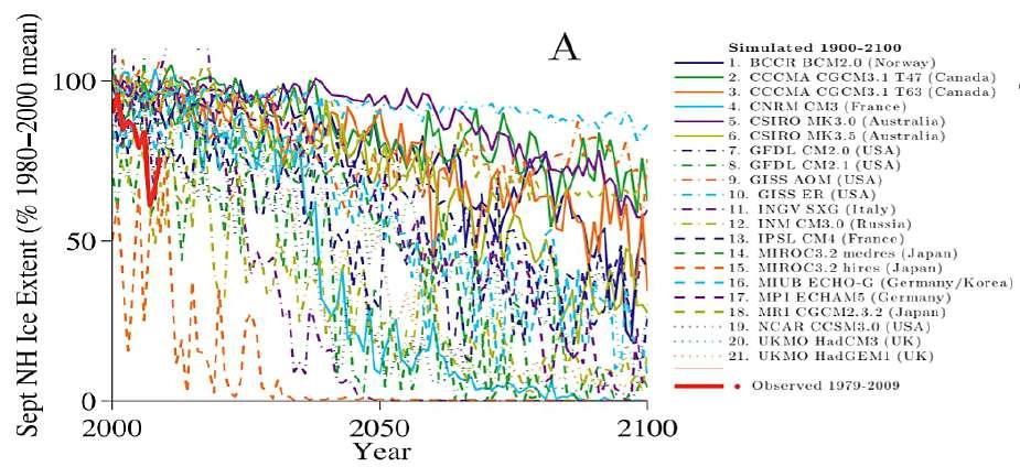
Figure 83. Differences among the GCM projections of the rate of Arctic sea ice loss. Timeline toward seasonally ice-free Arctic Ocean conditions indicated by Northern Hemisphere September sea ice extent during the twenty-first century scaled by the 1980–2000 mean September value for each model. From Eisenman et al. (2011).

As all geo-scientists have been knowing for a very long time, the Earth is a unique and extraordinarily complex system and Mother Nature is not impressed by a +0.007% (max) CO2 increase of its overall atmospheric composition (70 ppm)

and has many tricks in her sleeves. We have just seen here how changes in oceanic currents (THC / AMOC), sea surface temperature cyclical variations (AMO), atmospheric oscillations (NAO), cloud cover modulation and albedo variations, geothermal gradient and even a particular geodynamic context all contribute to the Arctic climate far more than a tiny increase in a trace gas. Most geologists with an experience on the field know that and Dr. Donald Eschman will have the final word: “Before I retired from my position as a geology prof I often took my students on field trips out to the glacial deposits exposed in gravel pits west of Ann Arbor. In one very large pit (Killins gravel on Scio Church Road) the pit had a two layered aspect. At the bottom was the well washed sand and gravel that was deposited as the Erie Lobe of the Wisconsinian ice sheet had retreated and the meltwater pouring off the front of the ice laid down thick and economically valuable outwash material. Must have been a time of ice retreat and presumably warmer climate. At a later time the ice readvanced over the outwash gravel and laid down a thinner but very obvious layer of clayey glacial till. The climate must have cooled to get the ice to re-advance and then the climate changed or stalled and the melting ice lobe dropped it’s load of till (everything from fine clay to crystalline Canadian boulders as big as a car) on top of the outwash deposits. It’s situations like this that always made me dubious of the notion that the climate could only change for the worse because of man’s actions. What could be more natural than climate change”. Dr. Donald Eschman