3.3.DO CLIMATE MODELS ACCOUNT FOR OBSERVATIONS?

«First, the computer models are very good at solving the equations of fluid dynamics but very bad at describing the real world. The real world is full of things like clouds and vegetation and soil and dust which the models describe very poorly. Second, we do not know whether the recent changes in climate are on balance doing more harm than good. The strongest warming is in cold places like Greenland. More people die from cold in winter than die from heat in summer. Third, there are many other causes of climate change besides human activities, as we know from studying the past. Fourth, the carbon dioxide in the atmosphere is strongly coupled with other carbon reservoirs in the biosphere, vegetation and top-soil, which are as large or larger. It is misleading to consider only the atmosphere and ocean, as the climate models do, and ignore the other reservoirs. Fifth, the biological effects of CO 2 in the atmosphere are beneficial, both to food crops and to natural vegetation. The biological effects are better known and probably more important than the climatic effects.» Freeman Dyson

As Lindzen stated (1997) «The more serious question then is do we expect increasing CO2 to produce sufficiently large changes in climate so as to be clearly discernible and of consequence for the affairs of humans and the ecosystem of which we are part. This is the question I propose to approach in this paper. I will first consider the question of whether current model predictions are likely to be credible. We will see why this is unlikely at best»

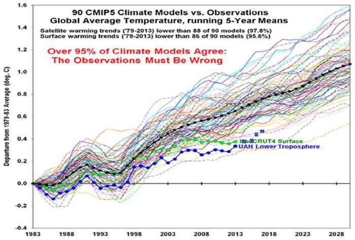
Models must be subordinated to the observations, not the other way round. This is the way science has always proceeded, for example when you compute the orbit of a double star (Poyet, 2017a; 2017b) if it does not match the observations you just try to recompute a better orbit. And every astronomer, given the method you have stated that you use, can have access to the observations, reproduce the work that you have done and check that it was correct. This is the very basics of science, the theory or the model should match the observations and science should be reproducible. As long as the theory or the model is able to make decent forecasts (i.e. an ephemeris in the previous example), it is considered appropriate, as soon as it fails, everything must be reconsidered. It seems that climate tinkerers have completely forgotten the basics and the observations must be wrong as 95% of the models fail to reproduce them, even on extremely short timescales as it is displayed in the next figure 99!

Figure 99. >95% of the models have over-forecast the warming trend since 1979, whether use is made of their own surface temperature dataset, i.e. HadCRUT4 (Morice et al., 2012), or of UAH satellite dataset of lower tropospheric temperatures. After Spencer (2014).

«Unfortunately, no model can, in the current state of the art, faithfully represent the totality of the physical processes at stake and, consequently, no model is based directly on the basic mechanical, physical or geochemical sciences. On the contrary, these models are fundamentally empirical and necessarily call on arbitrary parameters which must be

adjusted to best represent the existing climatological data, foremost among which is the annual cycle of the seasons » (Morel, 2009).282

From this benchmarking of the models against reality, Christy (2016) observes «On average the models warm the global atmosphere at a rate 2.5 times that of the real world. This is not a short-term, specially-selected episode, but represents the past 37 years, over a third of a century», this is well visible on next Figure 100. See also Gregory (2019).

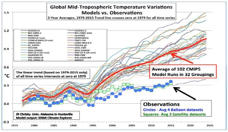
Figure 100. Global average mid-tropospheric temperature variations (5-year averages) for 32 models (lines) representing 102 individual simulations. Circles (balloons) and squares (satellites) depict the observations. The Russian model (INM-CM4) was the only model close to the observations (Christy, 2016).

Thus, as we explained before taking the example of the computation of the orbits of double stars, one will not be surprised by the conclusions logically drawn by Christy (2016) «Following the scientific method of testing claims against data, we would conclude that the models do not accurately represent at least some of the important processes that impact the climate because they were unable to “predict” what has already occurred. In other words, these models failed at the simple test of telling us “what” has already happened, and thus would not be in a position to give us a confident answer to “what” may happen in the future and “why.” As such, they would be of highly questionable value in determining policy that should depend on a very confident understanding of how the climate system works».

Back to our astrometric comparison, that means that these models, if they were orbits, would not even represent past observations data correctly, i.e. in fact they would be rejected immediately by the astronomer as he would know that no decent ephemeris could be derived of an orbit that does not even account for the past observations. This is the dire situation in which the climate science community stands after having received massive amounts of money with clear instructions while allocating the grants to prove that the temperature had to be explained by changes in [ CO2]. Could be time to revisit all assumptions. In astronomy, when you do not succeed to compute an orbit, there might be a third object, or else more. But at least you know that Kepler’s laws will stand, well they have been so far. Here, the Kepler’s law of the climate fiasco community, i.e. that everything depends on [CO2] concentration does not look so good, might be high time to change the gun instead of insisting on disregard for the obvious.

Furthermore, all these computer codes, their documentations and data used should be available in the public domain as they have been funded by tax-payer monies and as their authors cannot claim trade secrets to prevent their public availability. Even though this would be the case, which has not always been to say the least, the use of supercomputers could hamper the reproducibility of these experiments as stated by Laframboise (2016) «There is no reason to believe that the politically charged arena of climate science is exempt from these problems, or that it doesn’t share the alarming rates of irreproducibility observed in medicine, economics, and psychology. Indeed, non-transparency is an

282Pierre Morel, Oct. 2009, at «Bureau des longitudes». https://www.canalacademie.com/ida5110-Rechauffement-planetaire-etscience-du-climat.html

acute problem in climate science due to the use of climate modeling via supercomputers that cost tens of millions of dollars and employ millions of lines of code» and the reproducibility and assessment of the way the computers models operate is also legitimately challenged «Outsiders – whether they be other scientists, peer reviewers, or journalists –have no access to the specialized software and hardware involved, and it is difficult to imagine how such access might be arranged, never mind the person-years that would be required to fully explore the subtle computational and mathematical issues arising from a careful audit of such a model. Reproducibility is the backbone of sound science. If it is infeasible to independently evaluate the numerous assumptions embedded within climate model software, and if third parties lack comparable computing power, a great deal of climate science would appear to be inherently nonreproducible» (Laframboise, 2016).

Climate science is also characterized by a disproportionate usage of computer models as compared to other disciplines. In fact, and in some way, the software code has substituted itself to the very object of the study, the climate of planet Earth, and the modelers and software developers have come to believe that their creations are the real system, or so close of an image of it that one should not question the soundness, reliability or forecasting capacity of these systems. As Michaels and Wojick (2016) observe «in short it looks like less than 4% of the science, the climate change part, is doing about 55% of the modeling done in the whole of science. Again, this is a tremendous concentration, unlike anything else in science». Climate modeling is not climate science which furthermore does not really exist as we have seen before, inasmuch it is such a collection of disparate knowledge garnered from so many disciplines.

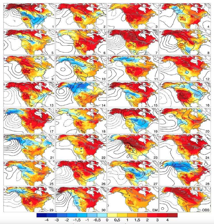
Figure 101. Computer models and chaotic results: Lorenz effect. 30 results of the same program which ran with initial conditions different from one thousandth of a degree Celsius: the trends over 1963-2013 of the surface temperatures in North America are represented, between -5°C (blue) and + 5°C (red). Down on the right EM (Ensemble Mean is the mean of the 30 runs) OBS is observed conditions. Image from Kay et al. (2015) and Snider (2016).

Moreover, the climate science research that is done appears to be largely focused on improving the models, i.e. an evasive virtual reality which is not so real unless you trust it! Michaels and Wojick (2016) add « In doing this it assumes

that the models are basically correct, that the basic science is settled. This is far from true. The models basically assume the hypothesis of human-caused climate change. Natural variability only comes in as a short term influence that is negligible in the long run. But there is abundant evidence that long term natural variability plays a major role climate change. We seem to recall that we have only very recently emerged from the latest Pleistocene glaciation, around 11,000 years ago. Billions of research dollars are being spent in this single minded process. In the meantime the central scientific question -- the proper attribution of climate change to natural versus human factors -- is largely being ignored».

The original legend of Fig. 21 by Snider (2016) was «Winter temperature trends (in degrees Celsius) for North America between 1963 and 2012 for each of 30 members of the CESM Large Ensemble. The variations in warming and cooling in the 30 members illustrate the far-reaching effects of natural variability superimposed on human-induced climate change. The ensemble mean (EM; bottom, second image from right) averages out the natural variability, leaving only the warming trend attributed to human-caused climate change. The image at bottom right (OBS) shows actual observations from the same time period. By comparing the ensemble mean to the observations, the science team was able to parse how much of the warming over North America was due to natural variability and how much was due to human-caused climate change. (© 2016 AMS.)».

As reminded by Hansen (2016), «Averaging 30 results produced by the mathematical chaotic behavior of any dynamical system model does not average out the natural variability in the system modeled. It does not do anything even resembling averaging out natural variability. Averaging 30 chaotic results produces only the average of those particular 30 chaotic results» and such a legend is just a deception. In the paper that produced this image, the precise claim made was: «The modeling framework consists of 30 simulations with the Community Earth System Model (CESM) at 1° latitude/longitude resolution, each of which is subject to an identical scenario of historical radiative “forcing” but starts from a slightly different atmospheric state. Hence, any spread within the ensemble results from unpredictable internal variability superimposed upon the forced climate change signal» (Kay et al., 2015).

In fact Snider (2016) acknowledges the chaotic nature of the results «With each simulation, the scientists modified the model's starting conditions ever so slightly by adjusting the global atmospheric temperature by less than one-trillionth of one degree, touching off a unique and chaotic chain of climate events» that it makes the legend associated to the experience totally unsubstantiated. By adding that «The result, called the CESM Large Ensemble, is a staggering display of Earth climates that could have been along with a rich look at future climates that could potentially be» Snider (2016) confesses that throwing dices would have been no different and that the software provides no idea whatsoever as to which final conditions one can actually expect. "We gave the temperature in the atmosphere the tiniest tickle in the model, you could never measure it, and the resulting diversity of climate projections is astounding" Deser said, see also (Deser et al., 2012). Deser added "It's been really eye-opening for people", yes indeed it is and shows how useless these systems are. At least we can compliment IPCC for one of the rare correct statement they made «The climate system is a coupled non-linear chaotic system, and therefore the long-term prediction of future climate states is not possible», IPCC – 2001 – TAR-14 – «Advancing Our Understanding», p. 771

A classical deception technique is to use models as if they were the observed reality, mixing up past observed data (but often arbitrarily corrected), extrapolated or tampered data and “points” resulting from oriented models in the same graphical representations283 to confuse people and make them believe that the AGW mass is said and that there is no question to be asked. Most of the time what is presented as an indisputable and irrefutable reality is just an unbelievable tinkering where the impact of so-called “assessed” climate response to natural and human-induced drivers - that nobody knows - is arbitrarily evaluated by means of statistical techniques hiding the tampering done to the data (e.g. through multiple regression) and further subtracted, then what they call the “forcings” which has no definition or reality whatsoever in Physics284. It is evaluated by a “simple climate model”, i.e. an ad-hoc piece of software that implements a naive thermal response to an arbitrary increase of CO 2 and further retrofitted to the data that they cannot otherwise account for, to finally use hundreds of variations of the so-called “forcings” to, in the end hopefully, reach the desired results!

Llyod's article (2012) boils down to a long plea to desperately try, in the pay of the men of the climate fabricators, to overturn an aphorism that fundamentally defines science, the one placed by Pierre-Augustin Caron de Beaumarchais in

283https://www.carbonbrief.org/analysis-why-scientists-think-100-of-global-warming-is-due-to-humans 284Please, find just one Physics Textbook (not a climatologist gibberish) that defines what a “forcing” is! This scam will be addressed hereafter and debunked in detail later.

the mouth of his fictional character, Figaro, in the Marriage of Figaro, a comedy in five acts, written in 1778, who enunciates “Les commentaires sont libres, les faits sont sacrés”, which means "Comments are free, facts are sacred".

The author in Llyod (2012) creates two groups of scientists, one resorting to ‘direct empiricism’ who consider facts sacred and deliver the respected University of Alabama in Huntsville (UAH) measurements based on raw satellite data checked against radiosonde data and “are treated as windows on the world, as reflections of reality, without any art, theory, or construction interfering with that reflection” and another group called ‘complex empiricists’ who simply reject the facts they dislike because these disprove their models by stating that all of the datasets, both satellite and radiosonde, were considered as theory-laden or heavily weighted with assumptions which is just ultimate bad faith. Thus, Llyod (2012) states “they held that understanding the climate system and the temperature trends required a combination of tools, including models, theory, the taking of measurements, and manipulations of raw data”. It's awesome, it just clearly states black on white that “understanding the climate” requires to make every effort to ensure that nothing contradicts the models, which makes sense as it is their bread and butter! Then Llyod (2012) goes on “As I will show, the philosophical clash between ‘direct’ and ‘complex’ empirical approaches is one basis of this long disagreement over the status of climate models and the greenhouse effect”. There is no philosophical clash, we just have on the one side a clever quakery and on the other a legitimate aspiration to keep doing science the way it has always been “facts are sacred" and would the models accommodate the data and as long as they would correctly some value will be placed in them, otherwise just change the models, the theory, everything but make no compromise with the facts. But as the arbitrary CO2 warming resemble more a religion that the logical outcome of a reasoned calculation as was done in the first part of this document, there is simply no way to discard the dogma, no way to recoup one's mind. Llyod (2012) further goes on asserting that the ‘complex empiricists’ claim that ‘‘We have used basic physical principles as represented in current climate models, for interpreting and evaluating observational data” (Santer et al., 2005, p.1555)”. In fact, the paper of Santer et al. (2005) is quite amazing as it simply states that if the data and observations do not match the models of the simulations, then they must be wrong ! “ On multidecadal time scales, tropospheric amplification of surface warming is a robust feature of model simulations, but it occurs in only one observational data set. Other observations show weak, or even negative, amplification. These results suggest either that different physical mechanisms control amplification processes on monthly and decadal time scales, and models fail to capture such behavior; or (more plausibly) that residual errors in several observational data sets used here affect their representation of long-term trends”.

What an inversion of Science published in Science !

And as if not enough, Lloyd (2012) adds “Note that this is the opposite of direct empiricism; the data are seen in terms of the theory and its assumptions... The evaluation of datasets is one where raw data are evaluated as plausible or acceptable based on their compatibility with certain theoretical or dynamic processes”. I remain speechless, flummoxed, cannot type on the keyboard any more! The observations do not fit the models or the simulations, they must be wrong, that was Figure 99 “95% of Climate Models agree: the observations must be wrong”!

Furthermore, one will not forget that the numerical approximation of partial differential equations having no formal solutions since 1822 (it has not yet been even proven whether solutions always exist in three dimensions and, if they do exist, whether they are smooth !) into opaque computer codes with lots of discretizations and parametrizations does not represent a physical phenomenon but somehow and very imperfectly tries to mimic a little what mother Nature performs at a highly different complexity level and has been doing so for billions of years. If these models do not match what Nature does and tells us so by the measurements made, we're not going to change mother Nature by tinkering and tweaking the measurements. It is totally delusional to keep going along with some feckless tampering of the data and hope for understanding and thus forecasting anything meaningful.

Let's come to the “forcings”: these neo-physical notions are totally meaningless concepts. Radiative Forcing (RF) is defined by Myhre et al. (2013), as “the change in net downward radiative flux at the tropopause after allowing for stratospheric temperatures to readjust to radiative equilibrium, while holding surface and tropospheric temperatures and state variables such as water vapor and cloud cover fixed at the unperturbed values” and Effective Radiative Forcing (ERF) “is the change in net TOA downward radiative flux after allowing for atmospheric temperatures, water vapour and clouds to adjust, but with surface temperature or a portion of surface conditions unchanged”. Furthermore and very interestingly, one should notice that there are multiple ways to compute these fantasies as Myhre et al. (2013) add “Although there are multiple methods to calculate ERF, Calculation of ERF requires longer simulations with more complex models than calculation of RF, but the inclusion of the additional rapid adjustments makes ERF a better

indicator of the eventual global mean temperature response... The general term forcing is used to refer to both RF and ERF”.

This is a truly new way of "doing Physics". Instead of observing the real world, trying to understand how it works and unveil laws that could make sense and check against data and consider the theory only correct as long as not invalidated by the observations, "IPCC neo-Physicists" have decided that they would define physically meaningless notions (e.g. RF, ERF) that would dictate to Mother Nature how she should respond, and for example for RF she will not be allowed to make any change except to the stratospheric temperature, holding all else constant! What a scam, especially as it is by the slight variations of H2O vapor at the TOA, both in content and altitude, and therefore changing the Outgoing Longwave Radiation (or radiative flux) emitted towards the cosmos that the Earth balances it energy budget. Telling Mother Nature what she is allowed to do, what she must hold constant or unchanged is just amazing. As just seen, in the RF case, the fact that the Earth is just allowed to readjust stratospheric temperature keeping all else fixed is telling a lot about the way these neo-Physicists have "re-invented" science. As Veyres (2020) reminds “Since radiative forcing is, by definition, neither observable nor measurable, people rely on computer rantings and take the average of the results of different computer programs, obviously all questionable. Radiative forcing is a calculation made in a virtual world, so virtual that it was arbitrarily increased by 50% by the IPCC between the 2007 report and the 2013 report without anything having changed much in six years”. All these stories of “radiative forcing by greenhouse gases” are nonsense and it is mainly the water vapor content of the upper troposphere – which obviously does not remain constant as no IPCC control button can hold it such - that determines and regulates the thermal infrared flux emitted by the globe to the cosmos (i.e. the Outgoing Long-wave Radiation) and not a warming of this upper troposphere. Their "models" which rely on neither observable nor measurable ad-hoc neo-physical quantities (how convenient, isn't it?) have also arbitrarily decided that the 0.007% increase of CO 2 was going to destroy the Earth's atmosphere equilibrium and that there is no need to check whether this has any sense, the simulations are more than enough to tell Mother Nature how she should comply!

What an inversion of Science!

For the readers who want to have a clearer picture of where the models stand after all these years of re-inventing the world, Flato and Marotzke et al. (2013), p. 743, were kind enough to us to tell the truth “Most simulations of the historical period do not reproduce the observed reduction in global mean surface warming trend over the last 10 to 15 years. There is medium confidence that the trend difference between models and observations during 1998–2012 is to a substantial degree caused by internal variability, with possible contributions from forcing error and some models overestimating the response to increasing greenhouse gas (GHG) forcing. Most, though not all, models overestimate the observed warming trend in the tropical troposphere over the last 30 years, and tend to underestimate the longterm lower stratospheric cooling trend”.

Finally the neo-scientists resort to some hijacking of real science by pretending that their models are based on “sound” physical principles whereas they mistreat or betray them. For example, Randall et al. (2007) state “ Climate models are based on well-established physical principles and have been demonstrated to reproduce observed features of recent climate (see Chapters 8 and 9) and past climate changes (see Chapter 6)”. Clearly, from what Flato and Marotzke et al. (2013), p. 743, reported above just six years later this is not the case. But Randall et al. (2007) p. 600 continue “One source of confidence in models comes from the fact that model fundamentals are based on established physical laws, such as conservation of mass, energy and momentum”. But every meteorological coupled circulation model does the same, they are very sophisticated pieces of software indeed, but they still cannot make any forecast beyond 15 days, not 15,000 years or 150,000 years! As if that was not enough, Randall et al. (2007) p. 596 resort to Newton to ascertain some legitimacy to their computerized fantasies “Climate models are derived from fundamental physical laws (such as Newton’s laws of motion), which are then subjected to physical approximations appropriate for the large-scale climate system, and then further approximated through mathematical discretization. Computational constraints restrict the resolution that is possible in the discretized equations, and some representation of the large-scale impacts of unresolved processes is required (the parametrization problem)”. May I dare to summarize to save the mind of poor Newton, we deal with approximations that are further approximated with unresolved processes that require parametrizations! What a mess! And one should have absolute confidence in that sort of science supposed to represent the sound basis for extraordinarily coercive social policies, preventing you from traveling to save the planet, ruining your most fundamental constitutional liberties, claiming that there is a social cost of carbon 285, the ultimate non-sense, and that you should pay the price to redeem your sins! There are no social costs whatsoever, there are only benefits

285https://en.wikipedia.org/wiki/Social_cost_of_carbon

and as Idso (2013) states “For a 300-ppm increase in the air’s CO2 content, for example, herbaceous plant biomass is typically enhanced by 25 to 55%, representing an important positive externality that is absent from today’s state-of-theart social cost of carbon (SCC) calculations. The present study addresses this deficiency by providing a quantitative estimate of the direct monetary benefits conferred by atmospheric CO 2 enrichment on both historic and future global crop production. The results indicate that the annual total monetary value of this benefit grew from $18.5 billion in 1961 to over $140 billion by 2011, amounting to a total sum of $3.2 trillion over the 50-year period 1961-2011. Projecting the monetary value of this positive externality forward in time reveals it will likely bestow an additional $9.8 trillion on crop production between now and 2050”. We walk on our heads, there are only benefits to have some more CO2, the gas of life. How could we become so wacky?

Finally and it looks by now more like humor than anything else, as if climate was not made first and foremost of precipitation, Randall et al. (2007) p. 591, 600, 601 tell us “There is considerable confidence that Atmosphere-Ocean General Circulation Models (AOGCMs) provide credible quantitative estimates of future climate change, particularly at continental and larger scales. Confidence in these estimates is higher for some climate variables (e.g., temperature) than for others (e.g., precipitation)”. Enjoy first the word “confidence” which defines this strange Physics and then take good notice that we do not know where it is going to rain (no wonder, nobodies does beyond two weeks) but we know what the temperature will be as suffice it to claim that more CO2 (+0.007% of the overall atmospheric composition, i.e. 70 ppm) will equal with A LOT warmer! What an interesting forecast, how much did we have to spend for that one?

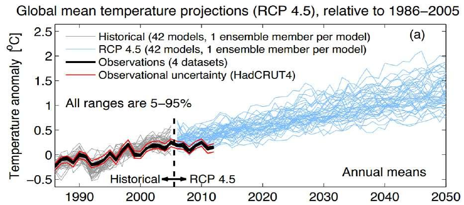
Figure 102. IPCC-AR5 Figure 11.9 | (a) Projections of global mean, annual mean surface air temperature 1986–2050 (anomalies relative to 1986–2005) under RCP4.5 from CMIP5 models (blue lines, one ensemble member per model), with four observational estimates: Hadley Centre/Climate Research Unit gridded surface temperature data set 3 (HadCRUT3); European Centre for Medium range Weather Forecast (ECMWF) interim reanalysis of the global atmosphere and surface conditions; Goddard Institute of Space Studies Surface Temperature Analysis; National Oceanic and Atmospheric Administration for the period 1986–2011 (black lines). Note that UAH data series are not among the data sets used. Source (IPCC, 2013), p. 981.

As one can see from the global mean temperature projections provided by (IPCC,2013), i.e. Figure 102, the ensemble model runs appearing here as a set of blue spaghettis are far from the observations that creep at the bottom of the graph, hardly taking off from the 0 (zero) level of the temperature anomalies and it will be explained that the models rendering the best the observations in this set are the various versions of the Institute of Numerical Mathematics of the Russian Academy of Sciences (INM RAS) Climate Model (CM). Before considering why the Russian models appear to perform much better than all the others, let's remind that when Randall et al. (2007) p. 600 state “One source of confidence in models comes from the fact that model fundamentals are based on established physical laws, such as conservation of mass, energy and momentum” they implicitly make reference to the Navier-Stokes equations, a set of partial differential equations which describe the motion of viscous fluid substances, and express conservation of momentum, conservation of mass, and conservation of energy. They are usually accompanied by an equation of state relating pressure, temperature and density. The Navier-Stokes equations are usually understood to mean the equations of fluid flow with a particular kind of stress tensor, but the GCMs do not really use Navier-Stokes equations. The base of

an atmospheric GCM is a set of equations called the “primitive equations”286. These represent conservation of momentum, the continuity equation (conservation of mass), the first law of thermodynamics (conservation of thermal energy) and lastly, an equation of state. If we track water vapor we need another continuity equation. The atmosphere can be assumed to be in hydrostatic equilibrium at the scales modeled, ~10-100 Km, i.e. the pressure-gradient force prevents gravity from collapsing Earth's atmosphere into a thin, dense shell, whereas gravity prevents the pressure gradient force from diffusing the atmosphere into space (hydrostatic balance can be regarded as a particularly simple equilibrium solution of the Navier–Stokes equations) or in quasi-hydrostatic state (models relax the precise balance between gravity and pressure gradient forces by including in a consistent manner cosine-of-latitude Coriolis terms), see Marshall et al. (1997). The ocean part is similar, but continuity amounts to zero divergence, because the ocean is taken to be incompressible. This set of hyperbolic partial differential equations is then discretized and solved by different means (Grossmann and Roos, 2007).

Then come phenomenons that cannot be taken into account at the grid level as they all occur at scales far below the “grid scale”, and thus are addressed differently and are often referred to as parametrizations (Hourdin et al., 2017) and include phenomenons such as condensation and precipitations, radiation and the way aerosols are taken into account e.g. Yu et al. (2018) for the NSF/DoE Community Earth System Model (CESM), friction, etc., and this is where the main intractable problems occur as these cannot follow in any respect physical laws, because either these laws are elusive or because we don’t know how to model them. Thus, the claim often made that GCMs are based on first-principle physics and primitive equations simply ignores the parameterizations and tuning above mentioned. If the models were truly based on physics, there would be no need for tuning, it would work properly ‘right out of the box’. This is why claiming that GCMs rests firmly on well established physical laws to impress the public is either an outright simplification or a more subtle deception.

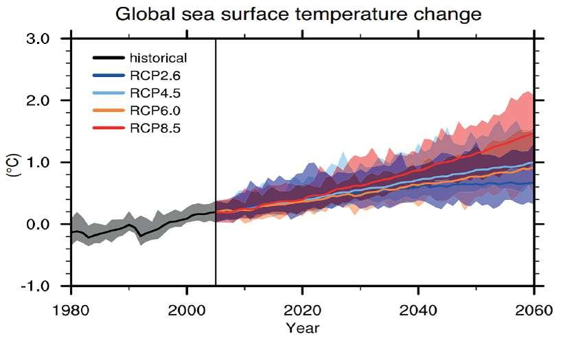
Figure 103. IPCC-AR5 Figure 11.19 | Projected changes in annual averaged, globally averaged, surface ocean temperature based on 12 Atmosphere–Ocean General Circulation Models (AOGCMs) from the CMIP5 (Meehl et al., 2007b) multi-model ensemble, under 21st century scenarios RCP2.6, RCP4.5, RCP6.0 and RCP8.5. Shading indicates the 90% range of projected annual global mean surface temperature anomalies. Anomalies computed against the 1986–2005 average from the historical simulations of each model. Source (IPCC, 2013), p. 993.

The excessive warming of the CMIP5 set of slow-cookers software fantasies is even acknowledged by IPCC (2013) “The discrepancy between simulated and observed GMST trends during 1998–2012 could be explained in part by a tendency for some CMIP5 models to simulate stronger warming in response to increases in greenhouse gas (GHG) concentration than is consistent with observations... Another possible source of model error is the poor representation of water vapour in the upper atmosphere... It has been suggested that a reduction in stratospheric water vapour after 2000 caused a reduction in downward longwave radiation and hence a surface-cooling contribution (Solomon et al., 2010), possibly missed by the models” Chapter 9, p. 771.

286The primitive equations are a set of nonlinear differential equations that are used to approximate global atmospheric flow and are used in most atmospheric models., they are atmospheric equations of motion under the additional assumption of hydrostatic equilibrium for large-scale motions. https://en.wikipedia.org/wiki/Primitive_equations for an introduction.

But the graph reproduced Figure 103, of the global sea surface temperature change forecasts does not appear much more convincing given the extremely large dispersion of the possible scenarios, and it will be reported by Frank (2019) that the situation is serious as the absence of a unique solution puts these models outside of the field of empirical science as they are simply not refutable (Popper, 1935, 1959; Sidiropoulos, M., 2019a-b) and as they do not portend any valuable information or forecast if considered how errors can cumulate over simulation cycles when they are correctly propagated and how they lead to unsustainable and extraordinary uncertainty ranges. In fact, the origin of the errors is multiple and Browning has a very long and extensive experience of the sources of error applying to numerical integration of formal set of equations (with special emphasis on symmetric hyperbolic sets of partial differential equations) having an application in meteorological or oceanic representations, e.g. Browning, et al. (1980, 1989), Browning and Kreiss (1986, 1994, 2002) and Browning (2020) using the mathematical Bounded Derivative Theory (BDT). Browning reminds that there are many sources of error in numerically approximating a system of time dependent partial differential equations and then using the numerical model to forecast reality.

He states that the total error E can be considered to be a sum of the following errors e i: E = ∑ ei: = DDE + SD + TD + F + ID where: • DDE, represents the error in the continuum dynamical differential equations versus the system that actually describes the real motion and contains errors from inappropriate descriptions of the dynamics, be they incorrect physical assumptions or too large of dissipative terms ; • SD, the spatial discretization (truncation) error is linked to the errors due to insufficient spatial resolution ; • TD, the time discretization (truncation) errors are due to insufficient temporal resolution; • F, the errors in the “forcing” (parameterizations versus real phenomena), these errors result from incorrect specification of the real forcing ; • ID, the error in the initial data.

It has been shown that SD and TD are not dominant for second order finite different approximations of the multi-scale system that describes large (1000 km) and mesoscale (100 km) features. Browning states “We have shown that these scales can be computed without any dissipation and it is known that the dissipation for these scales is negligible. It has been proved mathematically that the multi-scale system accurately describes the commonly used fluid equations of motion for both of these scales. We are left with F and ID and we have shown that F is large, e.g. the boundary layer approximation, and ID is large because of the sparse density of observations even for the large scale (Gravel et al., 2020). Thus there is no need for larger computers until F and ID are not the dominant terms”.

Currently all global climate (and weather) numerical models are numerically approximating the primitive equations (see note above 257), i.e. the atmospheric equations of motion modified by the hydrostatic assumption. But, Browning (2020) asserts that “It is well known that the primitive equations are ill posed when used in a limited area on the globe (…) this is not the system of equations that satisfies the mathematical estimates required by the BDT for the initial data and subsequent solution in order to evolve as the large scale motions in the atmosphere”, and reminds that the equations of motions for large-scale atmospheric motions are essentially a hyperbolic system, that with appropriate boundary conditions, should lead to a well-posed system in a limited area. The correct dynamical system is presented in the new manuscript of Browning (2020), and introduces a 2D elliptic equation for the pressure and a 3D equation for the vertical component of the velocity and goes into the details of why the primitive equations are not the correct system. Having done that, Browning (2020) can, in two short points, stress why the GCM relying on the wrong set of equations are inappropriate for any forecasting: • “Because the primitive equations use discontinuous columnar forcing (parameterizations), excessive energy is injected into the smallest scales of the model. This necessitates the use of unrealistically large dissipation to keep the model from blowing up (…) this substantially reduces the accuracy of the numerical approximation”; • “Because the dissipation in climate models is so large, the parameterizations must be tuned in order to try to artificially replicate the atmospheric spectrum. Mathematical theory based on the turbulence equations has shown that the use of the wrong amount or type of dissipation leads to the wrong solution. In the climate model case, this implies that no conclusions can be drawn about climate sensitivity because the numerical solution is not behaving as the real atmosphere”.

Of all the error terms listed above, Frank (2019) studies how just errors on F (and specifically tackling just one), when propagated throughout the simulation cycles of the software systems lead to valueless forecasts given the resulting uncertainty ranges. Frank (2019) starts from the ±4 Wm-2 cloud forcing error provided in Lauer and Hamilton (2013). Essentially, it’s the average cloud forcing error made by CMIP5-level GCMs, when they were used to hindcast 20 years

of satellite observations of global cloud cover (1985-2005). The differences between observed and CMIP5 GCM hindcast global cloud cover were published in Jiang et al. (2012). The difficulty to publish his manuscript has led Patrick Frank to wonder whether climate modelers are scientists. Frank (2015) stated “Climate modelers are not scientists. Climate modeling is not a branch of physical science. Climate modelers are unequipped to evaluate the physical reliability of their own models". The analysis of the tentative submission(s) and corresponding review reports shows that it is amazing to observe that beyond confusing accuracy with precision the reviewers also take an uncertainty range (resulting of the normal propagation of errors) for a potential physical temperature (anomaly). This paper has also led to a comprehensive exchange of arguments between Frank and Patrick Brown in Brown (2017). All that demonstrates that the entire climate-illusion beyond sloppy physics and moot modeling as reminded by Browning (2020) rests on GCMs that have no predictive value as explained by Frank (2019).

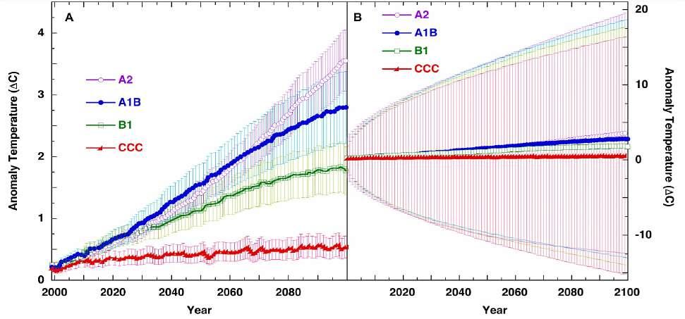
Figure 104. Panel (A), SRES scenarios from IPCC AR4 WGI Figure SPM.5 (IPCC, 2007) p.14, with uncertainty bars representing, the±1 standard deviation range of individual model annual averages. Panel (B) the identical SRES scenarios showing the ±1σ uncertainty bars due to the annual average ±4 Wm−2 CMIP5 TCF long-wave tropospheric thermal flux calibration error propagated in annual steps through the projections. After Frank (2009).

SRES in (A) refers to the IPCC Special Report on Emission Scenarios (Nakićenović et al., 2000; IPCC, 2000). Approximate carbon dioxide equivalent concentrations corresponding to the computed radiative forcing due to anthropogenic greenhouse gases and aerosols in 2100 (see p. 823 of the TAR) are the following for the various scenarios illustrated here: for the SRES B1 (600ppm), A1B (850ppm), A2 (1250ppm) and CCC corresponds to the case were the concentrations were held constant at year 2000 values. Figure 104 (B) shows the growing uncertainties resulting from the propagation of errors, i.e. the ±4 Wm-2 cloud forcing error as per Lauer and Hamilton (2013), due to the iterative process implemented in fact by any GCMs simulation software. This leads Frank (2019) to state “Uncertainty in simulated tropospheric thermal energy flux imposes uncertainty on projected air temperature” and conclude “The ±4 Wm−2 year−1 annual average LWCF thermal flux error means that the physical theory within climate models incorrectly partitions energy among the internal sub-states of the terrestrial climate. Specifically, GCMs do not capture the physical behavior of terrestrial clouds or, more widely, of the hydrological cycle (Stevens and Bony, 2013) ”. As shown on the previous Figure 104, the propagation of the long-wave cloud forcing (LWCF) thermal energy flux error through the IPCC SRES scenarios CCC, B1, A1B, and A2 leads to uncover a massive ±15 C uncertainty in air temperature at the end of a centennial-scale projection. An uncertainty should not be understood as a physical temperature range, it is the visible knowledge failure or uncertainty that results from the iterative propagation of just one of the many errors embedded in GCMs. Thus Frank (2019) asserts “Analogously large but previously unrecognized uncertainties must therefore exist in all the past and present air temperature projections and hindcasts of even advanced climate models. The unavoidable conclusion is that an anthropogenic air temperature signal cannot have been, nor presently can be, evidenced in climate observables”. If the reader believes that this affirmation is made on lightly further to Frank's (2019) paper, one is encouraged to read the extremely detailed answer provided by Frank to Patrick Brown in Brown (2017). More about models deficiencies along the same line of reasoning is presented in Hooper and Henderson (2016) and Henderson and Hooper (2017). A very complete study of the limitations of GCMs is provided by Lupo and Kininmonth (2013).

Of all the simulations performed during the Coupled Model Intercomparison Project Phase 5 (CMIP5) one can easily see from Figures 102 and 103 that models compare badly with observations and that little to no credence can be put into their future predictions. Among them, the INM RAS (Institute of Numerical Mathematics of the Russian Academy of Sciences) Climate Model 4, i.e. INMCM4 is an outliers, as it was certainly the one performing the best, not showing a totally unrealistic global warming as a response to GHG increase, though acknowledging many limitations (Figure 100). It is noticeable to observe the reasons behind this semblance of adherence to the observations:

1. INMCM4 has the lowest “sensitivity of 4.0 K to a quadrupling of CO2 concentration” (Volodin et al., 2013). That is 37% lower than multi-model mean; 2. INMCM4 has by far the highest climate system inertia and deep ocean heat capacity in INMCM4 is set at a value of 317 W yr m-2 K-1, which is a value situated at 200% of the multi-model average ; 3. INMCM4 exactly matches observed atmospheric H2O content in lower troposphere (at 215 hPa), and is biased low above that layer while most others are biased high.

So the model that most closely reproduces the temperature history has high inertia from ocean heat capacities, low forcing from CO2 and less water for unrealistic positive feedback. The obvious reason why other models are not designed like INMCM4 is that it does not support the man-made catastrophic story telling of IPCC of disastrous climate change resulting from CO2 increase. What is even more interesting is the appreciation of the authors the INMCM4 model, Volodin and Gritsun (2018) who state “Numerical experiments with the previous model version (INMCM4) for CMIP5 showed unrealistic gradual warming in 1950–2014”, therefore making it extremely clear, that what could be considered the best of all models, was not still evaluated as realistic by its own authors. The INMCM4 performances were detailed in Volodin et al. (2013). The evolution of INMCM4.0 lead to the INM-CM48 version with two major improvements: a) the use of more advanced parameterizations of clouds and condensation and b) interaction of aerosols with the radiation. Some other adjustment of other parameterizations were also performed. The next stage was to better model the stratosphere dynamics and its influence on the troposphere and was performed with the next generation INM-CM5 (Volodin et al., 2017; 2018; Volodin and Gritsun, 2018). Such model requires several hundred processors for the efficient computation on a supercomputer with distributed memory. Volodin et al. (2017) report “A higher vertical resolution for the stratosphere is applied in the atmospheric block. Also, we raised the upper boundary of the calculating area, added the aerosol block, modified parameterization of clouds and condensation, and increased the horizontal resolution in the ocean block” and the authors also focused on reducing systematic errors and phenomenons poorly handled or represented in previous versions.

Beyond the two main parts of such coupled ocean-atmosphere simulation systems, i.e. the general circulation of the atmosphere and of the ocean, the emergence of a generation Earth System Models (ESM) is based on the incorporation of other components of the climate system represented as additional software modules, e.g. models of the land surface (active layer, vegetation, land use), sea ice, atmospheric chemistry, the carbon cycle, etc. Hydrodynamics differential equations in the atmospheric module are solved in the quasi-static approximation with the finite difference method see e.g. Grossmann and Roos (2007) - which is of second order in space and first order in time, but Volodin et al. (2017) state that “Formally, there are no exact conservation laws in the finite difference model”. Compared to the INM-CM4 version, all resolutions are improved, the grid is finer and cells are 2° × 1.5° (longitude x latitude) and the vertical modeling contains 73 vertical levels with a vertical resolution in the stratosphere of about 500m, and the upper boundary of the calculating area lies at the altitude of about 60 km, about twice as much as in the previous version, and enables a much improved representation of the dynamics of the stratosphere. Within the cells, at the grid level, phenomenons are represented by parametrizations, i.e. atmospheric radiation, deep and shallow convection, orographic, and non-orographic, gravity-wave drag and processes in the soil, land surface, and vegetation. In the new INM-CM5 version the proportion of the cells occupied by clouds and cloud water content is calculated according to the prognostic scheme of Tiedtke (1993) for stratiform and convective clouds where their formation and evolution is considered in relation with the large-scale ascent diabatic cooling, boundary-layer turbulence, and horizontal transport of cloud water from convective cells and their disappearance is through adiabatic and diabatic heating, turbulent mixing, and depletion of cloud water by precipitation. In the GC ocean module, the hydrodynamics differential equations of the ocean are solved with the finite difference method on a generalized spherical coordinates grid with a resolution of 0.5° × 0.25° (longitude x latitude) and 40 levels vertically, using an explicit scheme for solving the transport equation with an iterative method for solving equations for the sea level and barotropic287 components of velocity.

287A barotropic fluid is a fluid whose density is a function of pressure only.

Volodin et al. (2017) explain that the explicit scheme was used as it opened possibilities to “adapt the algorithm of the model to massively parallel computers; The optimal numbers of processor cores for a given spatial resolution, as derived for the Lomonosov supercomputer in Moscow State University and supercomputer of the Joint Supercomputer Center of Russian Academy of Science, are 96 for atmospheric and aerosol blocks and 192 for the ocean block, i.e., 384 cores in total for the whole model. Under these conditions, the count rate is about 6 years of modeled time for one day of computer time”. Running such a system for a simulation spanning say 2,000 years, would take approximately an entire year of computing power of the most powerful Russian super-computers using 384 cores in parallel computing 288. This is a key information and it puts a lid on all claims made by any other author(s) or any other group(s) – e.g. (Lloyd, 2012) - that would pretend to succeed the modeling of the Holocene or more or would report such achievements! Volodin et al. (2017) have been extremely honest and have disclosed the state of the art of current Earth System Models with appropriate details and this entails much respect. A lot more information are provided by these authors about how they connect supplementary modules dealing with aerosols, ice-sheets, etc. and the frequency with which these modules are solicited by the parametrizations. The reader is encouraged to consider the following references: (Galin et al., 2007; Volodin, 2017; Volodin and Gritsun, 2018; Volodin et al., 2010, 2013, 2017, 2018).

Having been reminded that, Volodin and Gritsun (2018) put their INM-CM5 Earth System Model at work and perform seven historical runs for the 1850–2014, not the Holocene !, and provide a clear, honest and very informative report of where the best model stands so far. Here is what Volodin and Gritsun (2018) report “All model runs reproduce the stabilization of GMST in 1950–1970, fast warming in 1980–2000, and a second GMST stabilization in 2000–2014. The difference between the two model results could be explained by more accurate modeling of the stratospheric volcanic and tropospheric anthropogenic aerosol radiation effect (stabilization in 1950–1970) due to the new aerosol block in INM-CM5 and more accurate prescription of the TSI scenario (stabilization in 2000–2014)”. The authors also report the limitations encountered as simply no model trajectory reproduces the correct time behavior of the AMO and PDO indexes. From thereof they make very bold statements such as “the correct prediction of the GMST changes in 1980–2014 and the increase in ocean heat uptake in 1995–2014 does not require correct phases of the AMO and PDO as all model runs have correct values of the GMST, while in at least three model experiments the phases of the AMO and PDO are opposite to the observed ones in that time”.

Failing to account for the correct phases of the AMO and PDO and still getting some decent values for the GMST does not entail that there is no need to correctly model the AMO and PDO to obtain correct GMST. It just means that this very specific system gave the appearance of correctly modeling the temperature even though it was unable to render the state of the oscillations known to have a direct impact on the climate. Volodin and Gritsun (2018) further add “The North Atlantic SST time series produced by the model correlates better with the observations in 1980–2014. Three out of seven trajectories have a strongly positive North Atlantic SST anomaly as in the observations (in the other four cases we see near-to-zero changes for this quantity)”. It means that less than 43% of the runs, over just a total of 7, have managed to account for the SST anomalies. The worse deviation is for the the rate of sea ice loss which is underestimated by a factor between 2 and 3 with extreme dispersion as in one extreme case the magnitude of this decrease is as large as in the observations, while in the other the sea ice extent does not change compared to the preindustrial age. From all these runs with what seems the best state of the art system as it reasonably well account for the GMST, the natural strong internal variability of Arctic sea ice and internal variability of the AMO dynamics remain far beyond current science and technology.

Let's compliment Volodin and Gritsun for their achievements and their honest account of the strengths and weaknesses of their latest NM-CM5 Earth System Model. At the same time, failing to account for the major AMO and PDO oscillations does not reinforce credence into the proper representation of the climate system as accounting better for the GMST than others does not ensure that this is not the result of the providence. As reminded by Christy (2016) “a fundamental aspect of the scientific method is that if we say we understand a system (such as the climate system) then we should be able to predict its behavior. If we are unable to make accurate predictions, then at least some of the factors in the system are not well defined or perhaps even missing. [Note, however, that merely replicating the behavior of the system (i.e. reproducing “what” the climate does) does not guarantee that the fundamental physics are wellknown. In other words, it is possible to obtain the right answer for the wrong reasons, i.e. getting the “what” of climate right but missing the “why”.]”.

Said just slightly differently, understanding enables forecasting, science has always worked that way. As long as climate story tellers cannot forecast when and where the next drought, the next flood, the next heat-waves, the next El Niño,

288https://www.open-mpi.org/ Open Source High Performance Computing based on a A High Performance Message Passing Library.

etc., will happen, they just show that their understanding of the phenomenons they pretend to master so well that their computerized fantasies would be able to ascertain to a fraction of a degree the global temperature a century from now is just a fake propaganda designed to pursue a social engineering agenda, mind and population control, wealth redistribution, de-industrialization as a means to fight capitalism, etc., and that this has nothing to do with science. If they cannot say anything meaningful about the climate just a month from now, not a year or a decade or a century, no, just ONE month, their models, their computer systems and their gibberish is worthless, they should shut up.

It is interesting to note that scholars who have devoted an entire life to climate models and climate dynamics are starting to be extremely cautious with respect to the kind of expectations that one can have with climate simulation systems. In fact, the more they acknowledge the importance of natural climate variability the more they explain that the best forecasts they can expect of their systems is no forecast at all.

This trend started in 2010 with a paper from Deser et al. (2012) where the authors used the National Center for Atmospheric Research (NCAR) Community Climate System Model Version 3 (CCSM3) to evaluate how natural variability, i.e. the real climate, would affect the runs. Deser et al. (2010) assert “The dominant source of uncertainty in the simulated climate response at middle and high latitudes is internal atmospheric variability associated with the annular modes of circulation variability. Coupled ocean-atmosphere variability plays a dominant role in the tropics, with attendant effects at higher latitudes via atmospheric teleconnections”. Surprisingly enough, it is nearly acknowledged that the climate is not made of more or less of CO2, but of a vast number of systems interacting, though one can doubt that the simulator does represent them all and them well, and already in 2010, it was further stated that “ the Internal variability is estimated to account for at least half of the inter-model spread in projected climate trends during 2005–2060 in the CMIP3 multi-model ensemble”.

This cautious trend seems to be more and more in fashion as a recent paper by Maher et al. (2020) with Marotzke as co-author and studying the role of internal variability in future expected temperature start by acknowledging that “On short (15-year) to mid-term (30-year) time-scales how the Earth’s surface temperature evolves can be dominated by internal variability as demonstrated by the global-warming pause or ‘hiatus’”. Mentioning the 'hiatus' is also saying that the exponential increase of man-made CO2-emissions has not led to a monotonic or worse accelerated increase of the temperature, there has simply not been any relationship: when emissions where still limited a rapid increase (19221941) led to a top in the 40ties, then a stabilization of GMST in 1950–1970, fast warming in 1980–2000, and a second GMST stabilization in 2000–2014 (Akasofu, 2013) when emissions were accelerating fast, all that shows that GMST evolved independently of the rates of the anthropogenic emissions. As if experienced scholars were already doubting that the catastrophic changes or even very noticeable climate changes would over the next 30 years – or ever happen, Maher et al. (2020) state “We confirm that in the short-term, surface temperature trend projections are dominated by internal variability, with little influence of structural model differences or warming pathway. Finally we show that even out to thirty years large parts of the globe (or most of the globe in MPI-GE and CMIP5) could still experience nowarming due to internal variability”.

Finally, as for Deser et al. (2012) ten years before, the real climate system and its variability is back on stage in the foreground, relegating CO2 not to the second roles, nor even to the background but to no mention at all, and lately Maher et al. (2020) say “Additionally we investigate the role of internal variability in mid-term (2019-2049) projections of surface temperature. Even though greenhouse gas emissions have increased compared to the short-term time-scale, we still find that many individual locations could experience cooling or a lack of warming on this mid-term time-scale due to internal variability”. This is worth repeating what they dare say in this paper, that after we've been told by pundits that the tropics will have reached Paris (France) in 30 years, it seems now that some better advised scholars start preparing us to an eventual cooling for the next 30 years should things go astray, just in case natural variability plays a bad trick on them.

This trend continues with an honest paper co-authored by twenty leading scientists developing computer models of the climate where Deser et al. (2020) report of the extraordinary computing resources used for just one Large Ensemble (LE) “the CESM1-LE used 21 million CPU hours and produced over 600 terabytes of model output" to obtain modest results where it is stated that “Internal variability in the climate system confounds assessment of human-induced climate change and imposes irreducible limits on the accuracy of climate change projections, especially at regional and decadal scales".

As to the accuracy of the climate models or rather inaccuracies, they certainly diverge from reality when observed data is not assimilated to force them back towards reality, which is not surprising as meteorological forecasting systems do

the same when not put back on track every six hours or so. This has led Pielke (1998) to state “ This is one (of a number of reasons) that I have been so critical of multi-decadal climate predictions. They claim that these are different types of prediction (i.e. they call “boundary forced” as distinct from “initial value” problems), but, of course, they are also initial value predictions”. Rial et al. (2004) p. 30, do not appear more optimistic when it comes to climate prediction “our examples lead to an inevitable conclusion: since the climate system is complex, occasionally chaotic, dominated by abrupt changes and driven by competing feedbacks with largely unknown thresholds, climate prediction is difficult, if not impracticable. Recall for instance the abrupt D/O warming events (Figure 3a) of the last ice age, which indicate regional warming of over 10°C in Greenland (about 4°C at the latitude of Bermuda). These natural warming events were far stronger – and faster – than anything current GCM work predicts for the next few centuries. Thus, a reasonable question to ask is: Could present global warming be just the beginning of one of those natural, abrupt warming episodes,.. ?”.

As we have seen in the sections before, models also have a hard time to cope with the most basic short-term observations in a variety of domains, ranging from the modeling of the Arctic sea ice and its extent, as they are well known to overestimate Arctic warming (Huang et al., 2019) and produce as shown Figure 83 p.204, taken from Eisenman et al. (2011) ludicrous estimates used by the IPCC to forecast the summer minimum in Arctic sea ice in the year 2100 (relative to the period 1980–2000), but also fail among other severe weaknesses to account for the cooling that can be expected of the volcanic aerosols as reported by Chylek et al. (2020) who even state furthermore that solar variability is not even taken care of at all “The CMIP5 models also greatly underestimate the effect of solar variability on both hemispheres. In fact, in CMIP5 models there is effectively no influence of solar variability on temperature, while the analysis of the observed temperature suggests quite a significant effect, especially on the southern hemisphere, consistent with the global results of Folland et al. (2018)”. In fact, CMIP5 model just considerably overestimate the cooling that can be expected of volcanic aerosol, by 40-50% and Chylek et al. (2020) “hypothesize that the models' parameterization of aerosol‐cloud interactions within ice and mixed phase clouds is a likely source of this discrepancy ”. One should notice that by over-tuning in general the aerosol response of the models (thus exacerbating the cooling) and not taking into account the solar variability enables to over-emphasize the impact of CO 2 by exaggerating its warming effect. If one thinks that it happens by a fluke, I do not, and as explained before when so many parameters can be tweaked or tuned, it is no wonder that one finds a means to put CO2 at its expected place in the model adjusting its contribution and all others in hindcast.

A stunning recent study by Block et al. (2019) even shows, as far as the Arctic is concerned, that “ Climate models disagree on the sign of total radiative feedback in the Arctic” in fact, models and simulations are split and only half of them show negative Arctic feedbacks which implies that Arctic local feedbacks alone suffice to adjust in a stable way Arctic surface temperatures in response to a radiative perturbation, and Block et al. (2019) claims “ Our results indicate that the large model spread does not only arise from different degrees of simulated Arctic warming and sea ice changes, but also from the dependency of these feedback components to largely different and incoherent representations of initial temperatures and sea ice fractions in the preindustrial control climate which inversely relate to the exhibited model warming.” This not only does not provide a lot of confidence in the models and their results, but it also delivers a brilliant demonstration of what Peilke Sr. (1998) stated “In fact, multi-decadal climate predictions are claimed to be different types of prediction (i.e. called “boundary forced” as distinct from “initial value” problems), but, of course, they are also initial value predictions” and demonstrates the extreme fragility of such systems as large differences in initial sea ice cover and surface temperatures determine the increased spread in estimated warming.

And, if one is using a model that is either missing one or more non-trivial parameters, or if one or more parameters are wrong because of inaccurate measurements (or subsequent ‘corrections’) and the model is ‘tuned’ to get historical agreement, then the arbitrary adjustment provides no assurance that the adjustment will work beyond the interval of time used for tuning. That is, it becomes a process of fitting a complicated function to observational data that is only valid for a limited time interval; not unlike fitting a high-order polynomial and naively expecting predictions to be useful.

As the climate is first and foremost characterized by the precipitations as per Köppen-Geiger (Köppen, 1884a-b, 1936), a basic test to evaluate their relevance is to check the models against the precipitation records. This approach is followed by Anagnostopoulos et al. (2010) and also Koutsoyiannis et al. (2008) who propose a study with a special emphasis on the observed precipitations that “compares observed, long climatic time series with GCM-produced time series in past periods in an attempt to trace elements of falsifiability, which is an important concept in science (according to Popper, 1983, '[a] statement (a theory, a conjecture) has the status of belonging to the empirical sciences if and only if it is falsifiable')”. From thereoff, the authors observe that “At the annual and the climatic (30-year) scales,

GCM interpolated series are irrelevant to reality. GCMs do not reproduce natural over-year fluctuations and (…) show that model predictions are much poorer than an elementary prediction based on the time average. This makes future climate projections at the examined locations not credible”.

This strongly refutes the hypothesis that the climate can be deterministically forecast, that climate models could be used to such an endeavor and that this would make any sense to use these GCMs relying on hypothesized anthropogenic climate change to address the availability of freshwater resources and their management, adaptation and vulnerabilities as conjectured, e.g. by Kundzewicz et al. (2007, 2008). If climate models would rest on a comprehensive and satisfactory theory of climate, such a theory would describe exactly how climate responds to the radiative physics of GHGs: how convection reacts, how cloud properties and amounts are affected, how precipitations adjust, and so forth, all which to have been verified by direct comparison to accurate observations. Of course, none of this is available and has been done, and indeed does appear not possible, and none of this physics is known to be properly represented in the models.

Thus, one will not be disappointed by the dismal performance of the GCMs and by their inability to make any reliable forecast, especially with respect to the crucial aspect of precipitations which are at the core of climate. Most of this delusion comes from the fact that even though it is well agreed that the weather is chaotic and can only be forecast for a week or so, meteorological systems being constantly put back on track by means of all sets of observations, climate would be less as it would be more a boundary-forced system than an initial-value dependent problem.

It is interesting to observe how the official IPCC stance on that matter has evolved from 2001 where it was stated with some realism «The climate system is a coupled non-linear chaotic system, and therefore the long-term prediction of future climate states is not possible», IPCC – 2001 – TAR-14 – «Advancing Our Understanding», p. 771., to 2007 when unfortunately, this bout of lucidity has quickly vanished into the wispy streamers of the IPCC illusion machine and Randall et al. (2007) have peremptorily declared “Note that the limitations in climate models’ ability to forecast weather beyond a few days do not limit their ability to predict long-term climate changes, as these are very different types of prediction”, an unsubstantiated claim that would make climate predictable. This could not be further from the truth, and already some time ago Mandelbrot and Wallis (1969) offer investigative observational proof that such a claim is wrong: they looked at the statistics of 9 rainfall series, 12 varve series, 11 river series, 27 tree ring series, 1 earthquake occurrence series, and 3 Paleozoic sediment series and found no evidence for such a claim of distinctions between weather and climate.

Basically, Mandelbrot and Wallis (1969) p. 556-557 stated “That is, in order to be considered as really distinct, macrometeorology and climatology should be shown by experiment to be ruled by clearly separated processes. In particular, there should exist at least one time span λ, on the order of magnitude of one lifetime, that is both long enough for macro-meteorological fluctuations to be averaged out and short enough to avoid climate fluctuations. (…) It can be shown that, to make these fields distinct, the spectral density of the fluctuations must have a clear-cut “dip” in the region of wavelengths near λ, with large amounts of energy located on both sides. This dip would be the spectral analysis counterpart of the shelf in measurements of coast lengths. But, in fact, no clear-cut dip is ever observed. (…) However, even when the R/S pox diagrams are so extended, they still do not exhibit the kind of breaks that identifies two distinct fields.”

This means in plain English that if the weather is chaotic, the climate is as well, and we all know the weather is chaotic. Chaotic or not, one thing for sure, GCMs “predictions” are so out of sync with the observations that it makes them completely unsuitable for establishing any policies based on their fantasies. It is amazing to observe that in the same document where Randall et al. (2007) tout the ability of GCMs “to predict long-term climate changes” they also state that “Models continue to have significant limitations, such as in their representation of clouds, which lead to uncertainties in the magnitude and timing, as well as regional details, of predicted climate change” Randall, et al. (2007) p. 601. That deserves an award: how to say one thing and its contrary 170 pages apart in the same document. The “parametrization” of the clouds remains one the absolute weaknesses of the GCMs and this aspect is well covered, e.g. by Pielke, Sr., et al., (2007); Stevens and Bony (2013); Tsushimaa and Manabe (2013). Even though some progresses have been recently reported in that respect one should notice that cloud representation and parametrization remain highly prone to arbitrary adjustments as reported, e.g. by Muench and Lohmann (2020) “The simulated ice clouds strongly depend on model tuning choices, in particular, the enhancement of the aggregation rate of ice crystals”.

In the end, it is worth noticing that Monckton of Brenchley et al. (2015a-b) propose a much simpler model than the GCMs which does not fare worse than their very sophisticated counterparts, the pieces of software supposed to be the

ultimate weapons in climate-story telling. The model of Monckton of Brenchley et al. (2015a-b) is based on simple equations such as 83, and 84 and a low atmospheric sensitivity to CO2 and though criticized by many stands perfectly the comparison. In some sense, this demonstrates that our imperfect knowledge of the carbon cycle is built into defective Earth Systems Models (ESMs) which produce the atmospheric CO2 concentrations from different emissions scenarios that General Circulation Models (GCM, or climate models) use as input and Millar et al. (2017) have shown that the ESMs contribute to current models not only running too hot but simply astray.

Along the lines small is beautiful, some simple models succeed very well at reconstructing the Average Global Temperature (AGT), and compare more than favorably with much more sophisticated and opaque pieces of software characterized by their obscure operating intricacies, like CGMs. In that respect, studying the respective influence of Water Vapor (WV) and CO2, Pangburn (2020) states and demonstrates how “WV increase has been responsible for the human contribution to Global Warming with no significant net contribution from CO 2”. WV in the aforementioned study is the result of clear sky water vapor measurements over the non-ice-covered oceans in the form of total precipitable water (TPW)289. These measurements have been made since 1988 by Remote Sensing Systems (NASA/RSS) and use microwave radiometers to measure columnar (atmospheric total) water vapor, thanks to the properties of the strong water vapor absorption line near 22 GHz (RSS, 2020).

Pangburn (2020) asserts that “Humanity’s contribution to planet warming is from increased atmospheric water vapor resulting nearly all from increased irrigation. The increased CO2 has negligible effect on warming. Climate Sensitivity, the temperature increase from doubling CO2, is not significantly different from zero”. Pangburn (2018) studies how well AGT can be reconstructed by means of a simple algorithm employing clear observable variables which increments annually over the period of study. The algorithm uses three factors to explain essentially all of AGT change since before 1900. Pangburn (2018) selects “ocean cycles, accounted for with an approximation, solar influence quantified by a proxy which is the SSN290 anomaly and, the gain in atmospheric water vapor measured since Jan, 1988 and extrapolated earlier using measured CO2 as a proxy”. The approach in the analysis is ‘top down’ where, instead of trying to account for multiple contributing pieces, the behavior of the system as a whole is examined in response to the selected contributing factors. Using input data through 2018, the results of the analysis in order of importance of the contributing factors and their approximate contributions to the temperature increase 1909 to 2018 are: 1) the (increase in) water vapor TPW, 60% 2) the net of all ocean Sea Surface Temperature (SST) cycles which, for at least a century and a half, has had a period of about 64 years, 22% and 3) the influence of variation of solar output quantified by the SSN proxy, 18%. This simple methodology provides temperature reconstructions which match closely (96+%) the observations. The model could be supplemented with additional observable variables would reliable time-series be available, like the cloud cover, the sensitivity to which is discussed in Pangburn (2015), e.g. “Sustained increase of only about 1.7% of cloud area would result in an eventual temperature decline of 0.5 °C”.

The conclusion of Pangburn (2018) is well worth it, especially as it could prove correct, “Humanity has wasted over a trillion dollars in failed attempts using super computers to demonstrate that added atmospheric CO 2 is a primary cause of global warming and in misguided activities to try to do something about it. An unfunded engineer, using only a desk top computer, applying a little science and some engineering, discovered a simple equation that unveils the mystery of global warming and describes what actually drives average global temperature”.

Let's see how Tennekes (2009) after a prolific and remarkably successful career 291 summarizes his position: “Since heat storage and heat transport in the oceans are crucial to the dynamics of the climate system, yet cannot be properly observed or modeled, one has to admit that claims about the predictive performance of climate models are built on quicksand. Climate modelers claiming predictive skill decades into the future operate in a fantasy world, where they have to fiddle with the numerous knobs of the parameterizations to produce results that have some semblance of veracity.” and “Climate models cannot be verified or falsified (if at all, because they are so complex) until after the fact. Strictly speaking, they cannot be considered to be legitimate scientific products”.

289One should notice that there is no contradiction with the decrease of the RH at the TOA developed at point 1) p. 68 as what is considered here is the Total Precipitable Water (TPW) for the entire column of air, which does not prevent variations to occur in the vertical distribution of water vapor in the column – of course, and thus changes of the level at the TOA where water vapor radiates towards the cosmos, which has come down slightly (though total TPW has increased). 290Sun Spot Numbers as a proxy for the Sun activity, i.e. the time-integral of sunspot number anomalies. 291https://en.wikipedia.org/wiki/Hendrik_Tennekes