Modeling and Forecasting Sites for Affordable Housing in New York City to Meet Local Need

Author : Ar. Vaidehi Raipat

Co-Authors : Abdul aziz Alaql, Dan Levine, La-Toya Niles, Neeraja Narayanswamy, Utkarsh Atri, Vittorio Costa

Vaidehi Raipat, an Urban Data Scientist and an Architect is the Founder and Principal of Innovature Research and Design Studio [IRDS], Bangalore. She also works as a Consultant for Groundwork Data, New York, and Transit intelligence, Bangalore. She is also a fellow at HOW Institute, Bangalore. Her interests are in the field of Temporal, Social and cultural research and the use of such Data for public problem-solving. These data-driven ideologies drive her work as a consultant and also the agenda of IRDS. She has written, presented, and published many papers in National as well as International Journals.

Abstract :

Affordable housing is a pressing concern in New York City and the city must focus resources to best meet local needs. This study tests several models for the locations that have gained affordable housing under the Housing New York plan and the number of units at each location, based on the parcel attributes and neighborhood demographics. A random forest classifier and regressor are shown to slightly outperform, respectively, a logistic regression and a generalized linear model. The best-performing models are used to forecast sites of future affordable housing and the number of units expected at each parcel if it were developed as affordable housing. These forecasts are compared to localized need for housing, measured by 311 inquiries. These models can aid the city in focusing resources on neighborhoods with the greatest housing need and projecting the scale of affordable development at particular locations.

Keywords : Affordable Housing, Housing Development, Neighborhood, Demographics

Introduction

Affordable housing is a pressing and increasingly urgent concern in New York City. For years, the New YorkCity Department of Housing Preservation and Development (HPD) has redeveloped thousands of vacant lots that were transferred to its possession during the 1970s and early 1980s. Despite these efforts, according to the NYC Department of City Planning there has been about a 7.5 % increase in new housing units since 2010 . With the supply of HPD -owned land mostly depleted, the City must utilize other governmentowned land to maximize housing opportunities for New York households in need of affordable housing.

In New York City and across the country, cities are turning to underutilized real estate to create affordable housing. With the reduction of travel for leisure and for work, the Covid-19 pandemic created a new inventory for reconstruction, hotels, office buildings, and garages that are up for sale. In addition to these spaces, there are school campuses with extra land, police precincts and libraries that could be reconstructed as opportunities for new affordable housing and upgraded public amenities. There is a growing need for housing units for the homeless, extremely low-income, and low income individuals and it is unclear if existing programs can match the demand.

This project studied the locations of affordable homes created or preserved under New York City’s Housing New York program. We model the locations of sites and number of units based on parcel-level attributes and neighborhood demographics. We use these models to forecast. where additional housing is likely under existing City programs and policies. We then compare the forecast with local indicators of the need for affordable housing. These models can inform City decisions about areas where more housing is needed and specific plans for individual sites.

Data

We used several open data sources for this analysis, including PLUTO data on all New York City properties, U.S. Census data for neighborhood demographics, records of Housing New York properties, and 311 inquiries regarding affordable housing. Details on our data sources are included in Appendix

Our data consisted of several categorical variables (e.g. building class, zoning), which were converted into dummy columns. The result was a wide data set with 419 total features.

For classification tasks (detailed below), which considered every parcel, we used 213-vintage data to fit models, then used the newest PLUTO records (from 2021) and newest reliable data Census ACS data (from 2019) to forecast future development.

For regression of the number of units, which was trained only on parcels that have actual Housing New York units, we compiled PLUTO and ACS data specifically for the year before each project was started and used this for training. For forecasts, we used the same most current PLUTO and ACS data.

Methods

Classification

The first task we pursued was to build a model of the parcels which would have Housing New York affordable housing units, based on the unique parcel and building factors as well as the demographics of the surrounding neighborhoods. We employed several classification models for this task, training each on a subset of the data and testing on withheld training data to compare model performance.

Logistic Regression

We created a baseline classification model using Logistic Regression. To adjust for imbalanced data (a challenge detailed below), in this baseline model, we undersampled the overrepresented class to remove the imbalance and then used this data set to train and test our model. Results for our baseline model are shown in Table 1 .

Because of the expected multicollinearity among features, we tested using principal components in the logistic regression. This model performed slightly better after using PCA , but the improvement was not good enough to offset the loss of interpretability of features. So we ended up discarding that particular approach. Results for the logistic regression model using PCA are shown in Table 1 .

floor area ratio and total Black population, but the model does not quantify which is more important (the first and second splits were also performed b y the trend features). The importance of a feature can be computed by checking all the splits in which the feature was used and how much it has reduced the Gini index compared to the original node. Based on this method, the two most important features here are total Black population and median income (see Figure 1 ).

Figure 1 : Decision tree model

The recall performance of random forest classification was 0.89 and that of the decision tree was 0.88 , making random forest the best model amongst the classifiers we tested. Usually, a tree based model is used where features and outcomes are non-linear and/or where features interact with each other. We used the tree based model to check how the features in our model interact with each other. However, it is possible that in our model some features may b e completely independent of each other.

Handling imbalanced data

In the classification problem we faced a challenge of imbalanced data. Our data exploration identified a large imbalance in the data between the parcels that do have Housing New York units (n = 3,655 ) and those that do not (n= 671,026). We tested different ways to handle this imbalance.

The problem with training our model using the original imbalanced data is that when the count of a certain class overwhelms another class, the classifier may be biased toward that class. For example, imagine that we have a very “stupid” classifier that predicts no affordable housing on every parcel. Since the data is so imbalanced, this classifier will have a very high accuracy, as shown below.

Optimizing accuracy would miss the purpose of this task, predicting parcels that would have affordable housing. We instead measured performance on recall, or the portion of positive labels that are correctly predicted. We tested two approaches for balancing the training data set: undersampling the majority class and oversampling the minority class to have perfectly balanced data (i.e., same size for both label classes).

Random Forest

We additionally employed a random forest classification and decision tree to model whether parcels would have affordable housing units. This decision tree used 26 features with the cutoff point selected to minimize the variance or Gini index of the classes. This model selected as trend features

Testing levels of undersampling

To test whether the model could retain a reasonable level of recall performance while using more of the true negative samples, we fit and tested the model at 10 different sample sizes, ranging from a sample of the true negatives equal to the number of true positives, up to the complete data of true negatives. The recall dropped rapidly a s the sample size increased, falling below 50 percent when the true negatives numbered ten times the true positives (see Figure 2 ). This recall value can be compared to the baseline ratio of the portion of true positives in the full data, which is just 0.5 percent, and by this formal measure the model performs above baseline. However, making correct predictions of a parcel status less than 50 percent of the time is insufficient for the intended purpose of predicting future housing production.

The table highlights the possible gains in performance by using SMOTE. In particular, logistic regression showed slightly better performance when using SMOTE, but only in some instances (the random process yields slightly different results on different instances). The Decision Tree classifier has a 5.1% higher recall score by using SMOTE instead of the undersampling of the majority class. However, with the random forest classifier, SMOTE performed worse than undersampling, decreasing recall from 0.90 recall to 0.87.

After testing SMOTE oversampling independently, we used GridSearchCV to find the best combination of parameters across all six models. The best performance was shown on Decision Tree with SMOTE, with a recall score of 0 .9 4 . The best parameters found were: {‘max_depth’:2 , ‘max_leaf_n o des’:20}. This best model was used for later forecasting.

Regression

Figure 2 : Recall score a t different sampling levels. X-axis measures the ratio o f the size o f the sample o f true negative values (the larger class) to the number o f true positive values (the smaller class) (Log scale)

Using undersampling, we were limited to a very small sample of the data. We resolved bias problems, but leaving out so many data points comes with the risk of losing important relevant information for the prediction.

Oversampling the smaller class

As an alternative approach, we also oversampled the minority class by “creating” new parcels that are affected by affordable housing. Even though we are preventing any information loss, there could be overfitting on the duplicated data points from the original undersampled class. To solve this problem, we could create synthetic data points that are similar to the ones in the undersampled class using the SMOTE technique.1 Table 2 shows the recall scores for three different models: Logistic Regression, Decision Tree, and Random Forest using both plain undersampling of the majority class and oversampling of the minority class by using SMOTE.

Our second main task was to fit a regression model for the number of affordable housing units on parcels that are Housing New York properties. Housing New York encompasses a variety of different building types at different scales, so the number of affordable units on a parcel which falls under this program varies widely. It is important to build a model for the number of units to understand which parcel and neighborhood factors influence the scale of a project and forecast the likely size of a project at a given location.

To train the regression model we used the actual number of units on Housing New York parcels as the outcome and the parcel and Census Tract features from the year before the Housing New York project was started as predictors. We trained the model on a subsample of the data and then tested model performance out-of-sample.

Poisson Regression

We fit a Generalized Linear Model with a Poisson regression model (to match the discrete numbers of units and the distribution of units, with most parcels having few units and a smaller number of parcels with large numbers of units (see Figure 3a). Each column was standardized. Because of the multicollinearity between features, regularization was needed when fitting the model. By testing on a validation subsample of the training data, we found an α of 372 to produce the best fit. This model had out-of-sample D2 of 0.642.

Principal components

To handle the potential multicollinearity and compress the data, we further tested regression based on principal component analysis. Evaluation of the explained variance added by each successive principal component revealed we would still need many dimensions for an adequate regression model. Both linear and Poisson models were fitted using principal components. Figure 3 shows how the Poisson model D 2 score improves with the number of components included, but plateaus just below 0.60 .

Random forest regression

We further fit a random forest regression to predict the unit count. This model used the same features as the generalized linear model. The optimizing criterion was the reduction in Poisson deviance, to match the criterion used on the generalized linear model. The model was fit with expansive parameters (no minimum depth, minimum samples to split = 2, minimum samples at leaf = 1). This model performed slightly better in explained deviance than the generalized linear model, with a D 2 score o f 0.686. Table 3 compares model performance.

Measuring supply vs. demand

Overall, performance of the regression models was only mediocre. It may be that, with just a few thousand actual projects to model from there were insufficient samples and the models were undertrained.

Because of this, we determined it would not be feasible to further segment the data to regress for the numbers of units of particular types, sizes, or classes. Nonetheless, with our best model accounting for two-thirds o f the possible variation in the total number of units, we proceeded with a forecast for the number of units.

Forecast from 2021 data through classification and regression models

After finding optimal models on past data (and determining that these models performed reasonably well), we used the best-performing models for forecasts. We input current data for each feature, for each parcel, to forecast which parcels were likely to have Housing New York units and how many units would be likely on each parcel if that parcel were developed as affordable housing.

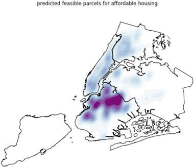
The predicted parcels were mapped to show which areas had more candidate parcels for affordable housing and the spatial distribution of the number of parcels. A kernel-density estimator (“heat map”) was plotted to show the spatial concentration of parcels classified as likely to host affordable housing (see Figure 4 ).

Forecast unit counts were also mapped and are shown to b e quite heterogeneo us, even at small scale. These fine-grained differences can be important for decision support.

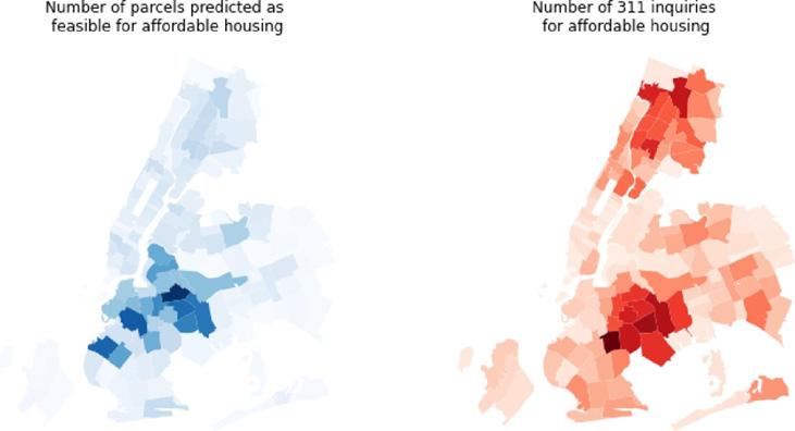
We used 311 inquiries about affordable housing as a measure of local need for housing. To compare forecast supply and demand, we summed both 311 requests and parcels by ZIP code areas, standardized each count (i.e., computed standard deviations from the mean for each value for each area), and took the difference in standardized values. Areas with positive values have a greater-than-typical number of inquiries for affordable housing compared to the number of local parcels forecast to be suitable for affordable housing. average, than their portion o f 311 inquiries would recommend (See Figure 6 ).

Discussion

Our classification forecast shows which parcels are likely to be developed as affordable housing, based on the parcel and building attributes and neighborhood characteristics. Because our classification models were trained on artificially balanced data, they projected these balanced proportions onto the forecast data. Our classifier forecast 192,664 parcels as more likely to be developed as affordable housing. This is an unrealistic total number of projects (considering fewer than 4,000 have been developed in the past eight years), but the locations and concentrations of these parcels are meaningful. We interpret the neighborhoods that have many parcels marked as likely for affordable housing to be those with more suitable sites for development. It is notable that even under a hypothetical scenario where nearly onequarter of properties in the City would be developed, very few sites on Staten Island or eastern Queens would likely gain affordable housing (see Figure 4 ).

We find a large degree o f alignment between the likely locations for affordable housing and the areas with the greatest demand (expressed through 311 inquiries) (see Figure 5 ).

However there are areas where local demand surpasses the proportional supply. This mismatch is particularly evident in East New York, southwest Queens, and the central Bronx (see Figure 6 ).

The difference between the inquiries and likely parcels for affordable housing align with the newly released Disparity Risk Index. These locations have an intermediate- to high risk for displacement and generally have a higher rent burden than the rest of the city.

The parcel-specific forecast of the number of expected units if a parcel were to be developed shows overall patterns but also high local variability (see Figure 7 ). Further spatial analytic tools could determine the exact spatial structure of these data.

Conclusion: to ward a decision support tool

The forecasts of likely locations for affordable housing development and parcel-level predictions of the expected number of units can aid the City in planning affordable housing sites. The difference between forecast number of suitable parcels and expressed need show which neighborhoods may need extra focus to find more sites for affordable housing.

Residents in the neighborhoods we identify with a housing deficit are also at a higher risk of displacement. In order for households in these neighborhoods not to be displaced in the years ahead, the City will need to utilize government-owned land and repurpo se underutilized property to maximize housing opportunities. With the limited availability of City owned land in these regions, the legislation before the State Assembly could further expand the landscape of options for affordable housing (i.e. the use of basements, garages, hotels, and office space for affordable housing).

These projects are capital intensive, To produce the current rate of housing preservation and new construction HPD expends over a billion dollars annually in capital. The FY2023 capital plan totals $1.43 billion. Under the 2023-2026 FourYear Plan, HPD has 4 .3 billion to conduct preservation and new construction activities.3 This allocation will allow the agency to keep pace with previous years, but it will not result in increased production. As a result, there is an even greater need to optimize the total number of units that can be produced. This will help to prioritize where new affordable housing development request for proposals (RFPs) should be issued.

The predicted number of units indicates the likely scale of a project a t any given location. This parameterized model could be used for ‘ what-if’ and optimization scenarios, e.g. considering how rezoning a parcel or combining or splitting parcels to change the developable size would affect the likely number of units.

https://equitableexplorer.planning.nyc.gov/about