Rit LbhÍ nr 34

FINAL REPORT

„Effects of lighting time and lighting source on growth, yield and quality of greenhouse sweet pepper“

Rit LbhÍ nr. 34

Christina Stadler

„Effects of lighting time and lighting source on growth, yield and quality of greenhouse sweet pepper“ FINAL REPORT Christina Stadler

Final report of the research project

„Effects of lighting time and lighting source on growth, yield and quality of greenhouse sweet pepper“

Duration: 15/07/2009 – 31/12/2010

Project leader: Landbúnaðarháskóla Íslands

Reykjum

Dr. Christina Stadler

810 Hveragerði

Email: christina@lbhi.is

Tel.: 433 5312 (Reykir), 433 5249 (Keldnaholt)

Mobile: 843 5312

Collaborators: Magnús Ágústsson, Bændasamtökum Íslands

Hjalti Lúðvíksson, Frjó Quatro ehf.

Knútur Ármann, Friðheimum

Sveinn Sæland, Espiflöt

Dr. Mona-Anitta Riihimäki, HAMK University of Applied Sciences, Finland

Dr. Carolin Nuortila, Martens Trädgårdsstiftelse, Finland

Project sponsor: Samband Garðyrkjubænda

Bændahöllinni við Hagatorg

107 Reykjavík

Framleiðnisjóður landbúnaðarins

Hvanneyrargötu 3

Hvanneyri

311 Borgarnes

Table of contents

SUMMARY

2 INTRODUCTION

MATERIALS AND METHODS

Greenhouse experiment

Lighting regimes

Measurements, sampling and analyses

Statistical analyses

RESULTS

4.1 Environmental conditions for growing

4.1.1 Solar irradiation

Photosynthetically active radiation and air temperature

Soil temperature

Irrigation of sweet pepper

Development of sweet pepper

4.2.1 Height

Number of fruits on a plant

Distance between internodes

4.3 Yield

4.3.1 Total yield of fruits

Marketable yield of fruits

Total fruit set

Outer quality of yield

4.3.5 Interior quality of yield 27

4.3.5.1 Sugar content

4.3.5.2 Taste of red fruits 28

4.3.5.3 Dry substance of fruits 28

4.3.5.4 N content of fruits 29

4.3.6 Dry matter yield of stripped leaves

4.3.7 Cumulative dry matter yield

4.4 Nitrogen uptake and nitrogen left in pumice

4.4.1 Nitrogen uptake by plants

4.4.2 Nitrogen left in pumice

4.5 Economics

4.5.1 Lighting hours

4.5.2 Energy prices

4.5.3 Costs of electricity in relation to yield

4.5.4 Energy use efficiency

4.5.5 Profit margin 39

Yield in dependence of light source

Yield in dependence of lighting time

Recommendations for saving

List of figures

Fig. 1: Experimental design of cabinets. 6

Fig. 2: Measurement points of photosynthetically active radiation and air temperature.

Fig. 3: Time course of solar irradiation. Solar irradiation was measured every day and values for one week were cumulated.

Fig. 4: Photosynthetically active radiation (solar PAR + PAR of lamps) and air temperature at different lighting regimes. PAR and air temperature was measured early in the morning at cloudy days.

Fig. 5: Soil temperature at different lighting regimes and different stem densities. The soil temperature was measured at little solar irradiation early in the morning.

Fig. 6: E.C. (a, c) and pH (b, d) of irrigation water (a, b) and runoff of irrigation water (c, d).

Fig. 7: Proportion of amount of runoff from applied irrigation water at different lighting regimes and stem densities.

Fig. 8: Water uptake at different lighting regimes and stem densities. 17 Fig. 9: Height of sweet pepper at different lighting regimes and stem densities. 18

Fig. 10: Relationship between height of sweet pepper and taken up water by sweet pepper plants at different lighting regimes and stem densities.

Fig. 11: Number of fruits (green and red) on the plant at different lighting regimes and stem densities.

Fig. 12: Cumulative total yield at different lighting regimes and stem densities. (1st class: > 100 g, too little weight: < 100 g). 21

Fig. 13: Time course of accumulated marketable yield at different lighting sources for interlighting and stem densities.

Fig. 14: Relationship between accumulated marketable yield and light intensity. 22

Fig. 15: Time course of accumulated marketable yield at different lighting times and stem densities.

Fig. 16: Time course of accumulated marketable yield at different lighting regimes and stem densities.

Fig. 17: Fruit set (fruit set (%) = (number of fruits harvested x 100) / total number of internodes) at different lighting regimes and stem densities.

Fig. 18: Sugar content of green and red fruits at different lighting regimes and stem densities.

Fig. 19: Dry substance of green (a) and red (b) fruits at different 28 lighting regimes and stem densities. 29

Fig. 20: N content of green (a) and red (b) fruits at different lighting regimes and stem densities. 30

Fig. 21: Dry matter yield of stripped leaves at different lighting regimes and stem densities. 31

Fig. 22: Cumulative dry matter yield at different lighting regimes and stem densities. 32

Fig. 23: Cumulative N uptake of sweet pepper (2 stems/plant). 33

Fig. 24: NO3-N and NH4-N in input and runoff water. 34

Fig. 25: NO3-N and NH4-N in pumice at the end of the experiment. 34

Fig. 26: Energy use efficiency in relation to lighting regimes and stem density. 39

Fig. 27: Revenues at different light sources and lighting times. 40

Fig. 28: Variable costs (without lighting and labour costs). 41 Fig. 29: Division of variable costs. 41

Fig. 30: Profit margin in relation to light sources and lighting times and stem density. 44

List of tables

Tab. 1: Irrigation of sweet pepper. 7

Tab. 2: Average distance between internodes and number of internodes at different lighting regimes and stem densities. 20

Tab. 3: Cumulative total number of marketable fruits (red and green) at different lighting regimes and stem densities. 25

Tab. 4: Proportion of marketable and unmarketable yield at different lighting regimes and stem densities. 26 Tab. 5: Lighting hours, power and energy in the cabinets. 35

Tab. 6: Costs and costs for consumption of energy for distribution and sale of energy. 37 Tab. 7: Variable costs of electricity in relation to yield. 38

Tab. 8: Profit margin of sweet pepper at different light sources and lighting times and stem densities (urban area, VA210). 42

Abbreviations

CaNO3 Calcium nitrate

DM dry matter yield

DS dry substance

E.C. electrical conductivity

H2O water

HPS high-pressure vapor sodium lamps

HSD honestly significant difference

IL interlighting

KCl potassium chloride

kWh kilo Watt hour

LED Light-emitting diodes

M mole

N nitrogen p ≤ 0,05 5 % probability level

PAR photosynthetically active radiation

pH potential of hydrogen TL top lighting

W Watt Wh Watt hours

Other abbreviations are explained in the text.

SUMMARY

In Iceland, winter production of greenhouse crops is totally dependent on supplementary lighting and has the potential to extend seasonal limits and replace imports during the winter months. Adequate guidelines for the most adequate lighting strategy (timing of lighting and light source) are not yet in place for sweet pepper production and need to be developed.

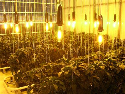
An experiment with sweet pepper (Capsicum annum L. cv. Ferrari, 9 stems/m2 and cv. Viper, 6 stems/m2) was conducted in the experimental greenhouse of the Agricultural University of Iceland at Reykir. Plants (two stems per plant, double rows) in four replicates were grown under HPS lamps for top lighting (160 W/m2) and either HPS lamps or LEDs (80 % 630 nm, 20 % 460 nm) for interlighting with comparable photosynthetically active radiation. Light was provided for max. 18 hours. During the time of high electrical costs for time dependent tariffs (December - February) one cabinet got supplemental light during the night as well during the whole weekend, whereas during the other months it was uniformly provided from 04 - 22 h as in the other cabinets, all the time. The weekly amount of light was equal in all cabinets.

Temperature was kept at 24 - 25 °C / 17 - 20 °C (day / night) and carbon dioxide was provided (800 ppm CO2). Sweet pepper received standard nutrition through drip irrigation.

The accumulated marketable yield of sweet pepper differed depending on the light source for interlighting and was about 20 % lower with LEDs. Also, the lighting time influenced accumulated marketable yield. When sweet pepper received light during nights and whole weekends marketable yield was 5 - 10 % lower compared to the normal lighting time. However, the yield continuously approached to the yield at normal lighting time when also here normal lighting time was used again. The yield increase was attributed to more fruits, whereas the average fruit weight was not influenced.

Marketable yield was 85 - 91 % of total yield and was lower with HPS interlighting compared to LED interlighting. This was mainly caused by a high percentage of burned fruits with HPS interlighting. It seems that fruits with blossom end rot are reduced with LEDs for interlighting and that sugar content and taste of fruits might have been better with HPS lamps.

There was no influence of the light source and lighting time on the distance between internodes. However, DM yield of stripped leaves, cumulative DM yield (yield of fruits, leaves, shoots) and N uptake by plants was increased with HPS lamps compared to LEDs.

Energy was converted less efficiently into yield with HPS lamps than with LEDs. The energy costs could be decreased by 25 % with LED interlighting, but only slightly with supplemental lighting during nights and weekends. However, the profit margin was highest with HPS lamps at normal lighting times. Possible recommendations for saving costs other than lowering the electricity costs are discussed.

At this stage, it is not recommended to change to LEDs. However, when LEDs have been adapted in future, environmental conditions must also be regulated according to the needs of LEDs. From the economic side it seems to be recommended to provide light at normal lighting times with HPS lamps.

INTRODUCTION

The extremely low natural light level is the major limiting factor for winter greenhouse production in Iceland and other northern regions. Therefore, supplementary lighting is essential to maintain year-round vegetable production. This could replace imports from lower latitudes during the winter months and make domestic vegetables even more valuable for the consumer market.

The positive influence of artificial lighting on plant growth, yield and quality of tomatoes (Demers et al., 1998a), cucumbers (Hao & Papadopoulos, 1999) and sweet pepper (Demers et al., 1998b) has been well studied. It is often assumed that an increment in light intensity results in the same yield increase. Indeed, yield of sweet pepper in the experimental greenhouse of the Agricultural University of Iceland at Reykir increased with light intensiy (Stadler et al., 2010). However, until the middle of April an increase from 240 (TL 120 + IL 120) to 280 (TL 160 + IL 120) W/m2 resulted in an increase of marketable yield of 13 % and an increase from 160 (TL 120) to 240 (TL 240) W/m2 resulted in an increase of 30 % (24/35 % with 6/9 stems/m2). At the lowest light intensity the accumulated marketable yield was not influenced by stem density. However, with higher light intensity the positive effect of a higher stem density was becoming obvious. Since the middle of April there was nearly no influence of different light intensities on marketable yield most likely because environmental conditions (temperature, illuminance) did nearly not differ within cabinets due to high solar irradiation. This fact makes it unnessessary to conduct lighting experiments at high natural light levels. Therefore, the present experiment was only runing until the end of April.

Traditionally, lamps are mounted above the canopy (top lighting), which entails, that lower leaves are receiving limited light. Both old and more recent experiments (HoviPekkanen & Tahvonen, 2008; Grodzinski et al., 1999; Rodriguez & Lambeth, 1975) imply that lower leaves are also able to assimilate quite actively, suggesting that a better utilization could be obtained by using interlighting (lamps in the row) in addition to top lighting. Indeed, the benefits from interlighting in contrast to top lighting alone have been confirmed with different vegetable crops. Interlighting increased first class yield of cucumbers along with increasing fruit quality and decreased unmarketable yield, both in weight and number (Hovi-Pekkanen & Tahvonen, 2008). However, in our experiment high-pressure vapor sodium lamps (HPS) were used for interlighting

and produced a lot of heat. When interlights were lowered and placed between the plants they caused burning on leaves and fruits. Marketable yield in the interlighting systems decreased, because 5 % of the fruits were damaged from lighting and blossom end rot increased by 2 % compared to the cabinets with only top lighing (Stadler et al., 2010).

HPS lamps are the most commonly used type of light source in greenhouse production due to their appropriate light spectrum for photosynthesis and their high efficiency. However, to lower or even to eliminate the damage on sweet pepper fruits from HPS interlighting the idea is based using interlighting lamps that are producing nearly no heat like light-emitting diodes (LEDs). LEDs have been proposed as a possible light source for plant production systems and have attracted considerable interest in recent years with their advantages of reduced size and minimum heating plus a longer theoretical life-span as compared to high intensity discharge light sources such as HPS lamps (Bula et al., 1991). Several plant species have been successfully cultured under LEDs (e.g. Avercheva et al., 2009; Tamulaitis et al., 2005; Schuerger et al., 1997; Brown et al., 1995; Hoenecke et al., 1992). These lamps are a radiation source with improved electrical efficiency (Bula et al., 1991) and nowadays one of the biggest advantages of LEDs seems to be their energysaving properties.

HPS lamps and LEDs differ in their spectral composition. The spectral output of HPS lamps is primarily in the region between 550 and 650 nm and is deficient in the IV and blue region (Krizek et al., 1998). With LEDs on the other hand, the ability to manipulate the spectral quality in LED lighting might offer a method of better plant growth and development. Spectral composition may indirectly affect plant nutrition (Ehret et al., 1989) and therefore it is necessary to evaluate also the N supply of plants by determining the N uptake and the input and runoff of the fertilization water.

Despite the increasing interest to alternative light sources other than HPS lamps, there is to the author’s knowledge not much information available that directly compares growth parameters and yield of vegetable crops grown at different light sources. Hence, one aim of this study is to investigate the growth, development and yield of a common horticultural greenhouse crop in Iceland, using sweet pepper as an example, traditionally grown under HPS lamps in comparison to LEDs and to determine the efficacy of these radiation sources. Even though the preliminary

experiment has shown a positive effect of a higher stem density at higher light intensities, again two stem densities will be tested, but with two varieties of sweet pepper - similar in growth -, grown at two different stem densities. The selection of two varieties and two stem densities will make the experiment more grower-related. It may be assumed that at different light sources an adaption of the plant density may be useful.

The costs for lighting are high, especially when growers are using electricity during the day and not during the night. Due to this “time dependent” tariffs, the idea was developed to lighten in cheaper times to decrease electricity costs. The sale for the energy is cheapest from 21.00-07.00 as well as on weekends and the distribution is lowest from 23.00-07.00 as well as on weekends. The energy is highest from 01.1101.03 from 09.00-21.00 in sale and from 07.00-23.00 in distribution. Therefore, to lower the energy costs it would be appropriate to lighten in the cheapest time, which is from 23.00-07.00 during weekdays and during weekends. However, the question arises, if sweet pepper would respond in growth, yield and quality in the same way, as the “usual” lighting time, which is each day from about 04.00-22.00. Hence, the main aim of this study is to test if there is a possibility to decrease lighting costs by lighting at cheaper times without a negative response of sweet pepper plants.

Incorporating lighting into a production strategy is an economic decision involving added costs versus potential returns. Therefore, the question arises whether different timings of lighting to decrease lighting costs are reflected in an appropriate yield of fruits and in a better energy use efficiency. In addition to different lighting times and light sources also stem densities will be considered with respect to the profit margin of the horticultural crops.

The objective of this study was to test if (1) different lighting times are affecting growth, yield and quality of sweet pepper and the N uptake of the plant, (2) decreasing energy costs by lighting at cheaper times are going along with an appropriate yield, (3) LEDs are appropriate to replace HPS lamps (4) the profit margin can be improved by lighting times and light sources. This study should enable to strengthen the knowledge on the lighting regime and give vegetable growers advice how to improve their sweet pepper production by modifying the efficiency of electricity consumption in lighting.

MATERIALS AND METHODS

3.1 Greenhouse experiment

An experiment with sweet pepper (Capsicum annum L.) was conducted at the Agricultural University of Iceland at Reykir. Seeds of sweet pepper were sown on 15.07.2009 in rock wool plugs. Seedlings were transplanted to rock wool cubes on 29.07.2009. On 27.08.2009 a pair of plants was transplanted in 11 l Bato-buckets (40 cm x 25 cm x 15 cm) filled with pumice stones and transferred to the cabinets with different lighting regimes.

Sweet pepper was trained to two stems per plant and was transplanted in double rows in four beds (A, B, C, D; Fig. 1). Two varieties of sweet pepper (Capsicum annum L. cv. Ferrari and cv. Viper) with a similar growth were chosen. But in contrast to Ferrari, Viper is more homogenous in growth. There were two stem densities (either 6 stems/m2 (Viper: B, D) or 9 stems/m2 (Ferrari: A, C)). Four replicates, i.e. two replicates in each bed consisting of four buckets (8 plants) acted as subplots for measurements (see packet in beds, Fig. 1). Other buckets (white, Fig. 1) were not measured and acted as a shelter belt.

Tab. 1: Irrigation of sweet pepper. Group Time of irrigation Duration between irrigations

Duration of irrigation Number of irrigations min min

IRRIGATION IN ALL CABINETS UNTIL THE END OF NOVEMBER 28.08.09-04.09.09 07.00, 13.30, 18.00 2.00 3 05.09.09-10.09.09 07.00, 11.00, 14.30, 18.00 3.00 4 11.09.09-22.09.09 07.00-19.05 180 2.00 5 23.09.09-30.11.09 06.00-21.05 150 2.30 7

IRRIGATION IN ALL CABINETS FROM DECEMBER UNTIL END OF FEBRUARY

Irrigation in all cabinets except “HPS, weekends” 01.12.09-09.12.09 06.00-21.05 150 2.30 7 10.12.09-17.12.09 9 18.12.09-19.01.10 11

Irrigation in cabinet “HPS, weekends” 01.12.09-17.12.09 20.00-07.00 120 2.30 6 18.12.09-08.01.10 20.00-07.00 120 2.30 7 09.01.10-20.01.10 20.00-09.05 60 2.30 14 21.01.10-11.02.10 20.00-16.00 60 2.00 21 12.02.10-02.03.10 20.00-08.00 45 1.30 17

Additional watering 01.12.09-11.01.10 13.00, 15.30 2.30 2 10.02.10-08.03.10 10.00-18.05 120 1.30 5

Watering at weekends

December, January 11.00, 18.00 2.30 2 February 6

Irrigation in cabinet “LED, 04-22”

20.01.10-08.02.10 05.00-21.05 90 2.15 11 09.02.10-01.03.10 05.00-21.05 45 1.30 22

Irrigation in cabinet “HPS, 04-22” and “HPS, 04-20/21/22” 20.01.10-08.02.10 05.00-21.05 60 2.00 17 09.02.10-01.03.10 05.00-21.05 45 1.45 22

IRRIGATION IN ALL CABINETS FROM MARCH UNTIL END OF APRIL 01.03.10-09.03.10 05.00-21.05 45 1.30* 1.45**, **** 22 10.03.10-16.03.10 05.00-21.05 35 1.20 * , 1.30**, **** 28 17.03.10-27.04.10 05.00-21.05 35 1.00 * , 1.10**, **** 28 03.03.10-27.04.10 05.00-21.05 35 1.30 *** 28

Additional watering 12.03.10-27.04.10 01.00 2.00*, **, ***, 1.30 **** 1

LED, 04-22

HPS, 04-22

HPS, weekends

HPS, 04-20/21/22

Temperature was kept at 24-25°C / 17-20°C (day / night) and ventilation started at 24°C. In contrast to the previous experiment temperature was higher and also the temperature difference between day and night, to be able to get taller plants with a bigger distance between internodes. Carbon dioxide was provided (800 ppm CO2 with no ventilation and 400 ppm CO2 with ventilation). A misting system was installed. Sweet pepper received standard nutrition (standard solution: 17,5 NH4 mmol / l) consisting of Calcium nitrate (CaNO3, 15,5 % N) and Bröste red (9 % N): 9,8 kg CaNO3 / 100 l H2O and 8,5 kg Bröste red / 100 l H2O) through drip irrigation (3 tubes per bucket). The watering was the following:

Plant cubes: 100 % CaNO3 : 70 % Bröste, until 1. setting: 100 % CaNO3 : 76 % Bröste, next 3 weeks 100 % CaNO3 : 100 % Bröste, until 2. setting: 78 % CaNO3 : 100 % Bröste, after 2. setting: 100 % CaNO3 : 100% Bröste.

E.C. was adjusted to 1,8-2,5 and pH to 5,5-6,5 depending on drainage E.C. and growth. Fertilizer application was kept the same in all cabinets until the end of November. After that the irrigation in cabinets differed (Tab. 1).

Plant protection was managed by using beneficial organisms and if necessary with insecticides.

3.2 Lighting regimes

Sweet pepper was grown until 26.04.2010 under high-pressure sodium lamps (HPS) for top lighting and either HPS lamps or LEDs for interlighting at four different lighting regimes with different timings of light, each in one cabinet:

1. HPS top lighting 160 W/m2 + LEDs interlighting 40 W/m2

- August to April: top lights and interlights from 04.00-22.00 (LED, 04-22) LED, 04-22

2. HPS top lighting 160 W/m2 + HPS interlighting 120 W/m2

- August to April: top lights and interlights from 04.00-22.00 (HPS, 04-22) HPS, 04-22

3. HPS top lighting 160 W/m2 + HPS interlighting 120 W/m2

- August to November: top lights and interlights from 04.00-22.00

- December and January: top lights from 20.00-09.00 and interlights from 13.00-16.00 and 19.00-09.00, top lights and interlights during weekends

- February: top lights from 20.00-09.00 and interlights from 19.00-08.00, top lights and interlights during weekends

- March and April: top lights and interlights from 04.00-22.00 HPS, weekends

4. HPS top lighting 160 W/m2 + HPS interlighting 120 W/m2

- August to November: top lights and interlights from 04.00-22.00

- December and January: top lights from 04.00-21.00 and interlights from 04.00-22.00

- February: top lights and interlights from 04.00-20.00

- March and April: top lights and interlights from 04.00-22.00

HPS, 04-20/21/22

HPS lamps for top lighting (600 W bulbs) were mounted horizontally over the canopy (4 m above ground) and HPS lamps (250 W bulbs) and LEDs (150 W, wavelength: 80 % 630 nm, 20 % 460 nm) for interlighting between plants in the rows regulated with plant height. However, until the end of November plants received only top lighting for 18 hours from 04.00-22.00 in all cabinets. After that, also interlighting was turned on and different lighting times started (see above): Whereas in two cabinets (1., 2.) light continued from 04.00-22.00, in the other cabinets (3., 4.) lighting time changed until the end of February with 18 / 16 hours light (December and January / February) in average. The hours of lighting were lower in February, because natural solar radiation increased. The total hours of lighting were comparable in these two cabinets. With the beginning of March all cabinets received again light from 04.0022.00. The lamps were automatically turned off when incoming illuminance was above the desired set-point.

3.3 Measurements, sampling and analyses

Soil temperature was measured once a week and air temperature and photosynthetically active radiation (subdivided between vertical and horizontal radiation) manually monthly at different vertical heights above ground (0 m, 0,5 m, 1,0 m, 1,5 m, 2,0 m) and at different horizontal positions (near the plant, between two plants, at the end of the bed, Fig. 2) under diffuse light conditions.

The amount of fertilization water (input and runoff) was measured every day and once a month the nitrate-N and ammonium-N of the applied water was analyzed with a Perkin Elmer FIAS 400 combined with a Perkin Elmer Lambda 25 UV/VIS Spectrometer.

To be able to determine plant development, the height of plants was measured each week and the number of fruits was counted each month.

Yield (fresh and dry biomass) of seedlings and their N content was analyzed. During the growth period, green and red fruits (> 50 % red) were regularly collected in the subplots each week. Total fresh yield, number of fruits, fruit category (1st class) and not marketable fruits was determined, each subdivided into red and green fruits. Additional samplings included stripped leaves during the growth period. At the end of the growth period on two plants (plants from one bucket) from the subplots the weight and the number of harvested and immature fruits and the number and distance of nodes was measured. The aboveground biomass of these plants was harvested and

points

Fig. 2: Measurement points of photosynthetically active radiation and air temperature.

divided into immature green fruits and shoots. For all plant parts, fresh biomass weight was determined and subsamples (three times for stripped leaves, green and red fruits) were dried at 105°C for 24 h for total dry matter yield (DM). Dry samples were milled and N content was analyzed according to the DUMAS method (varioMax CN, Macro Elementar Analyser, ELEMENTAR ANALYSENSYSTEME GmbH, Hanau, Germany) to be able to determine N uptake from sweet pepper.

In addition to regularly deformation analyzes, the interior quality of fruits was determined. A brix meter (Pocket Refractometer PAL-1, ATAGO, Tokyo, Japan) was used to measure sugar content in fruits at the beginning, in the middle and at the end of the growth period. From the same harvest, the flavour of fresh fruits was examined in tasting experiments with untrained assessors.

Composite soil samples for analysis of nitrate-N and ammonium-N were taken from buckets after transplanting and from the subplots at the end of the growth period. After sampling, soil samples were kept frozen. The soil was measured for nitrate (1,6 M KCl) and ammonium (2 M KCl) with a Perkin Elmer FIAS 400 combined with a Perkin Elmer Lambda 25 UV/VIS Spectrometer.

Energy use efficiency (total cumulative yield in weight per kWh) and costs for lighting per kg yield were calculated for economic evaluation of the light sources, also in interaction with varieties and lighting regimes.

3.4 Statistical analyses

SAS Version 9.1 was used for statistical evaluations. The results were subjected to one-way analyses of variance with the significance of the means tested with a Tukey/Kramer HSD-test at p ≤ 0,05.

4.1 Environmental conditions for growing

4.1.1 Solar irradiation

Solar irradiation was allowed to come into the greenhouse. Therefore, incoming solar irradiation is affecting plant development and was regularly measured. The natural light level decreased after transplanting into the cabinets continuously to < 5 kWh/m2 and was staying at this value to the middle of February 2010. However, with longer days solar irradiation increased naturally continuously to 15-30 kWh/m2 at the end of April 2010 (Fig. 3).

irradiation

3: Time course of solar irradiation. Solar irradiation was measured every day and values for one week were cumulated.

4.1.2 Photosynthetically active radiation and air temperature

Photosynthetically active radiation (PAR) is the photon flux within the spectrum of 400-700 nm. Plants are able to make use of this spectrum. In the case of the sweet pepper experiment solar radiation was allowed to come into the greenhouse and therefore, PAR and air temperature is composed of solar radiation and radiation of HPS lamps and LEDs and adjusted air temperature in the cabinets and heat of HPS lamps. LEDs are producing nearly no heat. To eliminate the incoming solar radiation

and the outside temperature, PAR and air temperature were measured early in the morning during cloudy days. The measured values for PAR and air temperature are converted into colours (red for high PAR / air temperature, yellow and white for low PAR / air temperature). This allows evaluating whether LED interlights are comparable to HPS interlights. The interlights were placed at measurement at about 1 m height, composing the PAR from the top lights. Naturally, these values are comparable within all cabinets (Fig. 4).

PAR

Air temperature

Lighting treatment

Measurement point above ground (m) between two plants near the plant at the end of the bed between two plants near the plant at the end of the bed

LED, 04-22 2,0

µmol/m2/s 1,5 350 - 999 1,0 300 - 349 0,5 250 299 0,0 150 - 249 100 - 149

HPS, 04-22 2,0 50 - 99 1,5 0 49 1,0 0,5 0,0

HPS, weekends2,0 °C 1,5 30,1-32,5 1,0 27,5-30,0 0,5 25,1-27,5 0,0 22,6-25,0 20,1-22,5

HPS, 04-20/21/222,0 15-20,0 1,5 1,0 0,5 0,0

Fig. 4: Photosynthetically active radiation (solar PAR + PAR of HPS lamps) and air temperature at different lighting regimes. PAR and air temperature was measured early in the morning at a cloudy day.

Also, the PAR that was affected by the interlight showed similar values for LED and HPS interlights, clarifying that both interlights are comparable regarding the light the plant can use. However, values were much higher at “HPS, 04-20/21/22”, because of a nearly absence of leaves due to spider mites, enabling the light to shine through. Stem density / variety did not influence radiation (data not shown). The temperature at the uppermost measurement points is lower with LEDs than with HPS interlights. This may be explained with the fact that HPS interlights produce head, irradiating also upper areas (Fig. 4).

4.1.3 Soil temperature

Soil temperature was mainly influenced by temperature of the heating pipe and was measured weekly at low solar radiation early in the morning. In December the heat was unstable and the cabinets could not be kept at the adjusted temperature. Soil temperature stayed most of the time between 20-24°C (Fig. 5). The soil temperature of “LED, 04-22” was most of the time lower than of “HPS, 04-22”. High values were measured in “HPS, 04-20/21/22” because of less leaves due to spider mites. Soil temperature was slightly higher at 6 stems/m2 compared to 9 stems/m2.

5: Soil temperature at different lighting regimes and different stem densities. The soil temperature was measured at little solar irradiation early in the morning.

standard

and are contained within the symbol if not indicated.

1,5 2,0 2,5

Viper, 6 Stems/m2 Ferrari, 9 Stems/m2 a

HPS, weekends HPS, weekends LED, 04-22 LED, 04-22 HPS, 04-22 HPS, 04-22 HPS, 04-20/21/22 HPS, 04-20/21/22

9.9.20097.10.20094.11.20092.12.200930.12.200927.1.201024.2.201024.3.201021.4.2010E.C. of applied water (mmhos)

Viper, 6 Stems/m2 Ferrari, 9 Stems/m2

HPS, weekends HPS, weekends LED, 04-22 LED, 04-22 HPS, 04-22 HPS, 04-22 HPS, 04-20/21/22 HPS, 04-20/21/22

pH of applied water

Viper, 6 Stems/m2 Ferrari, 9 Stems/m2

HPS, weekends HPS, weekends LED, 04-22 LED, 04-22 HPS, 04-22 HPS, 04-22 HPS, 04-20/21/22 HPS, 04-20/21/22

pH of runoff

9.9.20097.10.20094.11.20092.12.200930.12.200927.1.201024.2.201024.3.201021.4.2010

Viper, 6 Stems/m2 Ferrari, 9 Stems/m2

HPS, weekends HPS, weekends LED, 04-22 LED, 04-22 HPS, 04-22 HPS, 04-22 HPS, 04-20/21/22 HPS, 04-20/21/22

9.9.200930.9.2009

2.12.200930.12.200927.1.201024.2.201024.3.201021.4.2010

4.1.4 Irrigation of sweet pepper

E.C. and pH of irrigation water was fluctuating much (Fig. 6 a, b). E.C. ranged between 2 and 3 and pH between 5 and 7. E.C. of runoff increased during the growth period from 2 to about 4 (Fig. 6 c). PH of runoff decreased from 8 to 5 at the end of 2009 and increased after that to about 6 (Fig. 6 d). The amount of runoff from applied irrigation water was about 20-70 % (Fig. 7). The amount of runoff was lower for 6 stems/m2 than for 9 stems/m2. Highest values were measured for “LED, 04-22”.

6 Stems/m2

Amount of runoff from applied water

9 Stems/m2

weekends LED, 04-22 LED, 04-22 HPS, 04-22 HPS, 04-22 HPS, 04-20/21/22 HPS, 04-20/21/22

weekends

Fig. 7: Proportion of amount of runoff from applied irrigation water at different lighting regimes and stem densities.

With longer growing period taken up water by plants increased naturally (Fig. 8). Until the end of December plants took up approximately 2 l/m2. Thereafter, water uptake increased to 3-6 l/m2. Taken up water was lowest for the treatment “LED, 04-22”.

4.2 Development of sweet pepper

4.2.1 Height

Sweet pepper was growing about 0,5 cm/day and reached at the end of the experiment heights from 160 to 200 cm (Fig. 9). Plants with 6 stems/m2 were mostly significantly higher than with 9 stems/m2 With increasing height of sweet pepper water consumption rose (Fig. 10). The increment of taken up water was lowest for the treatment “LED, 04-22”.

6 Stems/m2 Ferrari, 9 Stems/m2

HPS, weekends

weekends LED, 04-22 LED, 04-22 HPS, 04-22 HPS, 04-22 HPS, 04-20/21/22 HPS, 04-20/21/22

Fig. 9: Height of sweet pepper at different lighting regimes and stem densities.

bars indicate standard deviations and are contained within the symbol if not indicated. Letters indicate significant differences at the end of the experiment (HSD, p ≤ 0,05).

Vip er, 6 Stems/m2 Ferrari, 9 Stems/m2

HPS, weekends HPS, weekends LED, 04-22 LED, 04-22 HPS, 04-22 HPS, 04-22 HPS, 04-20/21/22 HPS, 04-20/21/22

(cm)

Fig. 10: Relationship between height of sweet pepper and taken up water by sweet pepper plants at different lighting regimes and stem densities.

4.2.2

Number of fruits on a plant

The number of fruits on the plant was fluctuating between 20-60 fruits/m2 (Fig. 11). The number of fruits per square meter increased with a higher stem density. It seems that especially at the latter part of the growth period there were less fruits at “LED 04-22”. “HPS 04-22” was producing with “Viper” the highest amount of fruits compared to the other treatments, whereas with “Ferrari” the number seems to be similar in all treatments.

04-22

04-22

04-20/21/22

weekends

04-22

04-22

04-20/21/22

11: Number of fruits (green and red) on the plant at different lighting regimes and stem densities.

4.2.3 Distance between internodes

The distance between internodes was measured at the end of the growing season. The distance between internodes decreased with height (1st internode: counted from the division of the main stem into two stems), but from ca. 5th internode it stayed around 2-4 cm (data not shown). If the average distance between internodes and the number of internodes is examined no differences between lighting regimes and stem densities / varieties can be observed (Tab. 2). Also, the height of the main stem until the division into two stems did not differ between treatments (data not shown) and amounted 21-24 cm.

2:

Average distance between internodes and number of internodes at different lighting regimes and stem densities.

Light intensity Stem density

9

Stems/m2

9

Average distance between internodes in cm Number of internodes

HPS, weekends 4,0 a 3,8 a 45 a 44 a LED, 04-22 3,9 a 3,6 a 47 a 47 a HPS, 04-22 3,8 a 3,8 a 46 a 45 a HPS, 04-20/21/22 3,8 a 3,8 a 43 a 45 a Letters indicate significant differences (HSD, p ≤ 0,05).

4.3 Yield

4.3.1 Total yield of fruits

The yield of sweet pepper included all harvested red and green fruits and the green fruits at the end of the growth period. The fruits were classified in 1st class fruits (> 100 g/fruit), fruits with too little weight (< 100 g), fruits with blossom end rot, fruits with damage from lighting, not well shaped fruits, and fruits that were too mature and at the same time not mature. More than 50 % of the harvested marketable fruits were red. The proportion of red fruits was higher for “Ferrari” compared to “Viper”.

Cumulative total yield of sweet pepper ranged between 22-32 kg/m2 (Fig. 12). The two varieties gave a similar yield. However, at a higher yield level (HPS, 04-22; HPS weekends), Viper with 6 stems/m2 gave a tendentially higher yield compared to Ferrari with 9 stems/m2, whereas at a lower yield level (LED, 04-22), no variety / stem density dependent effect was observed. The light source influenced yield, HPS lights for interlighting resulted in a significant higher yield compared to LEDs for interlighting. Unnormal lighting times (night, whole weekends) during December until end of February reduced total yield significantly / tendentially (6 / 9 stems/m2). Spider mites in “HPS, 04-20/21/22” decreased yield (Fig. 12).

HPS, weekends

HPS, weekends

LED, 04-22

LED, 04-22

HPS, 04-22

HPS, 04-22

HPS, 04-20/21/22

HPS, 04-20/21/22

1. class, red

class, green too little weight, red too little weight, green not marketable, red not marketable, green

not marketable: blossom end rot, damage from lighting, not well shaped, too mature + not mature

Yield of sweet pepper (kg/m

Fig. 12: Cumulative total yield at different lighting regimes and stem densities. (1st class: > 100 g, too little weight: < 100 g).

Yield of too little weight was also not marketable, but classified as an extra group because there was a relatively high amount of these fruits. Letters indicate significant differences at the end of the harvest period (HSD, p ≤ 0,05).

4.3.2 Marketable yield of fruits

Marketable yield of sweet pepper differed depending on the light source for interlighting (Fig. 13). Interlights were turned on from the end of November until the end of the experiment (marked with yellow). The yield with HPS interlights (HPS, 04-22) was significantly / tendentially (6 / 9 stems/m2) higher than with LED interlights (LED, 04-22). The yield difference was 20 % less yield with LED interlights, which could be observed during the whole harvest.

The relationship between the accumulated marketable yield and the light intensity showed a yield advantage of a higher light intensity (if the Watts for HPS and LEDs are compared, but not their PAR value) and also the yield advantage of a higher stem density at a higher light intensity (Fig. 14).

13: Time course of accumulated marketable yield at different light sources for interlighting and stem densities. Letters indicate significant differences at the end of the harvest period (HSD,

between

Light was provided in all cabinets from 04.00-22.00, but lighting time differed between cabinets from the beginning of December to the end of February (marked with yellow, Fig. 15). The lighting time influenced marketable yield and was about 22 % lower when sweet pepper received light during night and whole weekends (HPS, weekends) instead of the normal lighting time. However, the yield of “HPS, weekends” was about 16 % lower before lighting times differed. Taking that into account, the yield decrease by lighting during nights and weekends would possibly be only about 5 %. When switched over to the normal lighting time at the beginning of March, the yield difference between these two treatments decreased continuously to 11 % and was comparable to the value at the beginning of the experiment. Therefore, the yield decrease was only fixed to the time where sweet pepper received light during nights and during whole weekends, but after that plants adapted to the normal yield and at the end of the experiment yield differences were not significant (Fig. 15).

15: Time course of accumulated marketable yield at different lighting times and stem densities.

Letters indicate significant differences at the end of the harvest period (HSD, p ≤ 0,05).

Marketable yield of weekly harvests differed between lighting regimes. Do to a spider mite problem in “HPS, 04-20/21/22” yield was until plants recovered (end of February) very low compared to the other cabinets (Fig. 16).

Fig. 16: Time course of marketable yield at different lighting regimes and stem densities.

Number of marketable fruits increased tendentially with a higher stem density / Ferrari (Tab. 3) and normal lighting time (HPS, 04-22). Not common lighting times (during night, weekends) decreased tendentially number of marketable yield compared to the normal lighting time. Also, LED interlighting resulted in a significant lower number of marketable fruits compared to HPS interlighting (Tab. 3).

The proportion of red fruits on marketable fruits was significantly higher at 9 stems/m2 / Ferrari (53-63 %) than at 6 stems/m2 / Viper (46-54 %) except for “HPS, 04-20/21/22”. More red fruits were harvested with LED interlighting compared to HPS interlighting (Tab. 2).

Average fruit size was consistently affected by stem density / variety. Red fruits were harvested with about 170-180 g / 140-150 g (Viper / Ferrari) and green fruits with about 140 g / 130 g (Viper / Ferrari) (data not shown).

Tab. 3: Cumulative total number of marketable fruits (red and green) at different lighting regimes and stem densities.

Lighting regime

of marketable fruits

density

of red fruits on marketable fruits

HPS, weekends 143 bcd 147 abc 47 de 59 abc LED, 04-22 122 d 140 bcd 54 bcd 63 a HPS, 04-22 161 ab 172 a 48 de 61 ab HPS, 04-20/21/22 132 cd 148 abc 46 e 53 cde

Letters indicate significant differences at the end of the harvest period (HSD, p ≤ 0,05).

4.3.3 Total fruit set

Total fruit set was calculated (fruit set (%) = (number of fruits harvested x 100) / total number of internodes) at the end of the harvest period and ranged from about

Stems/m2

Stems/m

Stems/m2 Stems/m

a a

Fig. 17: Fruit set (fruit set (%) = (number of fruits harvested x 100) / total number of internodes) at different lighting regimes and stem densities.

bars indicate standard deviations. Letters indicate significant differences (HSD, p ≤ 0,05).

40 to 80 %. Fruit set increased significantly with lower stem density / Viper except for “LED 04-22” (Fig. 17). LED interlighting reduced significantly the fruit set compared to HPS interlighting, whereas lighting during weekends and nights had only a minor influence on the fruit set.

4.3.4 Outer quality of yield

Marketable yield was about 81-91 % of total yield during the whole harvest period. Marketable yield was lower with HPS interlighting compared to LED interlighting (Tab. 4), which was mainly caused by burning of fruits. Especially, when light was turned on at the night and during the whole weekend, amount of unmarketable yield increased, because the harvest occurred directly after the weekend. Therefore, the amount of burned fruits could possibly be decreased by harvesting just before the weekend. It seems that fruits with blossom end rot are reduced with LEDs for interlighting in contrast to HPS for interlighting. Fruits with too little weight, not well shaped fruits as well as too mature and at the same time not mature fruits were comparable within lighting regimes. Also varieties showed differences: Ferrari was characterized by smaller fruits compared to Viper. In contrast, Viper had 2 % more fruits with damage from lighting. About 2 % more fruits at Viper were to mature or not mature and the fruits were then softer on one side. This is also one reason, why growers in the Netherlands stopped growing Viper.

Tab. 4: Proportion of marketable and unmarketable yield at different lighting regimes and stem densities.

regime Marketable yield

yield too little weight blossom end rot damage from lighting

not well shaped too mature + not mature

Interior quality of yield

Sugar content

Sugar content of red and green fruits was measured three times during the harvest period and increased with maturation of fruits from about 4 (green fruits) to about 7 °BRIX (red fruits) (Fig. 18). It seems that red fruits of Ferrari were sweeter than of Viper, causing significant differences, whereas this effect was not observed when fruits were green. LED interlighting seems to slightly reduce sweetness of red fruits (Fig. 18).

weekends

weekends LED, 04-22 LED, 04-22 HPS, 04-22 HPS, 04-22 HPS, 04-20/21/22 HPS, 04-20/21/22

18: Sugar content of green and red fruits at different lighting regimes and stem densities.

Error bars indicate standard deviations and are contained within the symbol if not indicated. Letters indicate significant differences at the end of the harvest period (HSD, p ≤ 0,05).

4.3.5.2

Taste of red fruits

The taste of red fruits, subdivided into sweetness, flavour and juiciness was tested by untrained assessors at the beginning (12.01.2010), middle (09.03.2010) and at the end (22.04.2010) of the harvesting period. Mainly, no differences in taste, sweetness, flavour and juiciness of red sweet pepper was found between different lighting regimes (data not shown). The rating within the same sample was varying very much and therefore, same treatments resulted in a high standard deviation. However, it seems that in the April testing Ferrari was tasting better than Viper and fruits from LED may had less flavour. There was no relationship between measured sugar content and sweetness of fruits at all tasting dates (data not shown).

4.3.5.3 Dry substance of fruits

Dry substance (DS) of fruits was measured three times during the harvest period. DS increased with maturation of fruits from about 6 % for green fruits to about 8 % for red fruits (Fig. 19). It seems that red fruits of Ferrari had less water than Viper.

04-22

04-22

04-20/21/22

04-22

04-22

04-20/21/22

HPS, weekends

HPS, weekends

LED, 04-22 LED, 04-22 HPS, 04-22 HPS, 04-22

HPS, 04-20/21/22 HPS, 04-20/21/2 2

Fig. 19: Dry substance of green (a) and red (b) fruits at different lighting regimes and stem densities.

Error bars indicate standard deviations and are contained within the symbol if not indicated. Letters indicate significant differences at the end of the harvest period (HSD, p ≤ 0,05).

4.3.5.4 Nitrogen content of fruits

N content of fruits was measured monthly and varied between 2,0-2,6 %. Neither differences in N content between green and red fruits nor between lighting regimes and stem densities were observed (Fig. 20).

a 0,0 0,2 0,4 0,6 0,8

Viper, 6 Stems/m 2 Ferrari, 9 Stems/m 2

HPS, 04-20/21/22 HPS, 04-20/21/2 2 HPS, 04-22 HPS, 04-22 LED, 04-22 LED, 04-22 HPS, weekends HPS, weekends

a a a

Viper, 6 Stems/m 2 Ferrari, 9 Stems/m 2

HPS, 04-20/21/22 HPS, 04-20/21/22 HPS, 04-22 HPS, 04-22 LED, 04-22 LED, 04-22 HPS, weekends HPS, weekends b

Fig. 20: N content of green (a) and red (b) fruits at different lighting regimes and stem densities.

Error bars indicate standard deviations and are contained within the symbol if not indicated. Letters indicate significant differences (HSD, p ≤ 0,05).

4.3.6

Dry matter yield of stripped leaves

During the growth period, leaves were regularly taken off the plant and the cumulative DM yield of these leaves was determined. DM yield decreased with stem density / variety Ferrari (except for HPS, 04-20/21/22) (Fig. 21). LEDs as interlights reduced yield significantly by about 50 % compared to HPS interlights. Unnormal lighting times slightly decreased dry matter yield. Spider mites in “HPS, 04-20/21/22” caused yield decrease (Fig. 21).

yield of stripped leaves

Fig. 21: Dry matter yield of stripped leaves at different lighting regimes and stem densities. Error bars indicate standard deviations and are contained within the symbol if not indicated. Letters indicate significant differences at the end of the harvest period (HSD, p ≤ 0,05).

4.3.7 Cumulative dry matter yield

The cumulative DM yield included all harvested red and green fruits, the immature fruits at the end of the growth period, the stripped leaves during the growth period and the shoots. Cumulative DM yield increased slightly with stem density / Ferrari (Fig. 22). LED interlighting reduced cumulative DM yield significantly compared to HPS interlighting. Lighting at nights and weekends did not affect the DM yield, but pests (HPS, 04-20/21/22) reduced yield. The ratio fruits on “shoots + leaves” was > 60 %.

Cumulative DM yield (g/m

green + red fruits stripped leaves shoots

a bc a abab bc

a c

HPS, 04- 20/21/22 HPS, 04-22 LED, 04-22 HPS, weekends HPS, 04- 20/21/22 HPS, 04-22 LED, 04-22 HPS, weekends

Fig. 22: Cumulative dry matter yield at different lighting regimes and stem densities.

Letters indicate significant differences at the end of the harvest period (HSD, p ≤ 0,05).

4.4 Nitrogen uptake und nitrogen left in pumice

4.4.1 Nitrogen uptake by plants

The cumulative N uptake included N uptake of all harvested red and green fruits, the immature fruits at the end of the growth period, the stripped leaves during the growth period and the shoots. The shoots and fruits contributed much more than the leaves to the cumulative N uptake (Fig. 23). Whether it was lightened from 04-22 or during nights and weekends did not influence N uptake. However, the light source had an effect on N uptake. LED interlighting significantly decreased N uptake compared to HPS interlighting.

N uptake (g 2N/m

Stems/m2

Fig. 23: Cumulative N uptake of sweet pepper (2 stems/plant). Letters indicate significant differences (HSD, p≤0.05).

4.4.2 Nitrogen left in pumice

The amount of NO3-N in input and runoff water was higher than the amount of NH4-N (Fig. 24). NH4-N amounted to be less than 100 and NO3-N most of the time around 300. While the amount of NH4-N was mostly lower in the runoff than in input water, the level of NO3-N was changing within input and runoff water during the growth period.

NH4-N and NO3-N in pumice were measured at the end of the experiment. NO3-N + NH4-N decreased slightly with a higher stem density (Fig. 25). It seems that the content was higher with LED interlighting and lighting at nights and weekends.

4.5 Economics

4.5.1 Lighting hours

The number of lighting hours is contributing to high annual costs and needs therefore special consideration in order to find the most efficient lighting treatment to be able to decrease lighting costs per kg marketable yield.

The total hours of lighting during the growth period of sweet pepper were both calculated and with dataloggers measured. The cabinet “HPS, 04-20/21/22” with the pest problem will be excluded for economic evaluation.

The calculated value was higher than the measured one, because in this value it was not included that lamps were automatically turned off, when incoming solar radiation was above the set-point and that interlights were turned off during harvest and during tending strategies (Tab. 5). The calculation of the power was higher for the measured values than for the calculated ones, because top lights at the outer beds were also partly contributing to lighten the shelter belt, whereas interlights were only placed within the experimental area. For calculation of the power different electric consumptions were made: one was based on the power of the lamps (nominal Watts, 0 % more power consumption), one with 6 % more power consumption for HPS bulbs and one for 10 % more power consumption.

Tab. 5: Lighting hours, power and energy in the cabinets.

Hours Power Energy Energy/m2 h W kWh kWh/m2 HPS, 04-22

Measured values 3420 356 60799 1216

Calculated values

0 % more power consumption (nominal) 3662 280 51264 1025 6 % more power consumption for HPS 3662 297 54340 1087 10 % more power consumption for HPS 3662 308 56390 1128 LED, 04-22

Measured values 3864 239 46085 922

Calculated values

0 % more power consumption (nominal) 4007 208 41674 833

6 % more power consumption for HPS 4025 218 43790 876 10 % more power consumption for HPS 4036 224 45202 904 HPS, weekends

Measured values 3418 356 60770 1215

Calculated values

0 % more power consumption (nominal) 3552 280 49721 944 6 % more power consumption for HPS 3552 297 52704 1054 10 % more power consumption for HPS 3552 308 54693 1094

4.5.2 Energy prices

Since the application of the electricity law 65/2003 in 2005, the cost for electricity has been split between the monopolist access to utilities, transmission and distribution and the competitive part, the electricity itself. Most growers are, due to their location, mandatory customers of RARIK, the distribution system operator (DSO) for most of Iceland except in the Southwest and Westfjords (Eggertsson, 2009).

RARIK offers basically three types of tariffs:

a) energy tariffs, for smaller customers, that only pay fixed price per kWh,

b) “time dependent” tariffs (Þrígjaldstaxti) with high prices during the day and winter but much lower during the night and summer, which mostly suites customers with electrical heating, but seem to be restricting for growers, and

c) demand based tariffs (Afltaxti), for larger users, who pay according to the maximum power demand (Eggertsson, 2009).

In the report, Þrígjaldstaxti and Afltaxti are used. The first type of tariff is not economic. Since 2009, RARIK has offered special high voltage tariffs (“VA410” and “VA430”) for large users, that must either be located close to substation of the transmission system operator (TSO) or able to pay considerable upfront fee for the connection.

Costs for distribution are divided into an annual fee and costs for the consumption based on used energy (kWh) and maximum power demand (kW) respectively the costs at special times of usage. The annual fee is pretty low, when subdivided to the growing area and is therefore not included into the calculation. Growers in an urban area in “RARIK areas” can choose between different tariffs. In the report only the possibly most used tariffs “VA210” and “VA410” in urban areas and “VA230” and “VA430” in rural areas are considered.

The government subsidises the distribution cost of growers that comply to certain criterias. Currently 67,0 % and 75,9 % of variable cost of distribution for urban and rural areas respectively. This amount can be expected to change in the future.

Based on this percentage of subsidy and the lighting hours (Tab. 5), for the cabinets the energy costs with subsidy per m2 during the time of the experiment that growers have to pay were calculated (Tab. 6).

Tab. 6: Costs for consumption of energy for distribution and sale of energy.

Costs for consumption Energy ISK/kWh

Energy costs with subsidy per m2 ISK/m2

HPS, 04-22 LED, 04-22 HPS, weekends real calculated real calculated real calculated real calculated real calculated real calculated

HPS, 04-22 LED, 04-22 HPS, weekends

DISTRIBUTION

67,0 % subsidy from the state VA210 1,04 1,01 1,01 1,01 0,99 0,98 0,97 0,97 1,04 1,02 1,02 1,02 1259 1037 1099 1140 909 814 854 880 1259 1018 1079 1120 VA410 0,84 0,81 0,81 0,81 0,79 0,78 0,78 0,78 0,84 0,82 0,82 0,82 1017 833 883 916 727 649 681 702 1017 820 869 902

RARIK Urban

RARIK Rural

75,9 % subsidy from the state VA230 1,06 1,03 1,03 1,03 1,01 1,00 1,00 1,00 1,06 1,05 1,05 1,05 1285 1061 1124 1167 933 836 877 905 1285 1040 1102 1144 VA430 0,64 0,63 0,63 0,63 0,61 0,60 0,60 0,60 0,64 0,64 0,64 0,64 783 643 681 707 561 502 526 543 783 632 670 695

SALE

Afltaxti Þrígjaldstaxti

3,57 4,67

3,49 3,49 3,49 4,66

3,39 4,58

3,36 3,35 3,35 4,59

3,58 3,57

3,53 3,53 3,53 3,64 1017 833 883 916 727 649 681 702 1017 820 869 902

Source: Composition from Eggertsson (2010)

Comments: The first number for the calculated value is with 0 % more power consumption, the second value with 6 % more power consumption and the last value with 10 % more power consumption for the HPS bulbs.

The energy costs per kWh for distribution after subsides are around 1 ISK/kWh for „VA230“ and „VA230“, around 0,8 ISK/kWh for „VA410“ and around 0,6 for „VA430“.

The energy costs for sale are for „Afltaxti“ around 3,5 ISK/kWh with less difference between cabinets and for „Þrígjaldstaxti“ around 4,6 ISK/kWh, but for „HPS, weekends“ around 3,6 ISK/kWh.

Not surprisingly the costs of electricity decreased with LED interlighting by about 25 % compared to HPS interlighting (Tab. 6). However, the costs for “HPS, 04-22” and “HPS, weekends” were comparable. With higher tariffs costs decreased.

4.5.3 Costs of electricity in relation to yield

Costs of electricity in relation to yield for wintergrown sweet pepper were calculated (Tab. 7).

Tab. 7: Variable costs of electricity in relation to yield.

Variable costs of electricity per kg yield ISK/kg

Lighting treatment HPS, 04-22 LED, 04-22 HPS, weekends

Stem density 6 9 6 9 6 9 Yield/m2 25,5 23,8 19,4 19,7 23,0 20,8

real calculated real calculated real calculated real calculated real calculated real calculated

Urban area (Distribution + Sale)

VA210 220 181 192 200 235 194 206 213 208 187 196 202 205 184 193 199 244 197 209 217 270 218 231 240 VA410 211 173 184 191 225 185 197 204 199 178 187 193 196 175 184 189 233 188 200 207 258 209 221 229

Rural area (Distribution + Sale) VA230 221 182 193 201 237 195 207 214 209 188 197 203 206 185 194 200 245 198 210 218 271 219 232 241 VA430 202 166 176 182 215 177 188 195 190 170 179 184 187 168 176 181 223 180 191 198 247 200 212 220

While for the distribution several tariffs were possible, for the sale the cheapest tariff was considered. The costs of electricity decreased with “LED, 04-22” by about 5-10 % compared to “HPS, 04-22”. Due to the lower yield of “HPS weekends” compared to “HPS, 04-22”, costs of electricity per kg yield increased by about 10-15 %. With a larger tariff, costs of electricity per kg yield decreased (Tab. 7). With the larger tariff there was a surprising advantage for rural areas, due to the subsidy distortion.

4.5.4 Energy use efficiency

Energy use efficiency is an indicator how efficient the kWhs are converted into yield, whereby a high value is showing better efficiency. The energy use efficiency was about 0,02 kg yield / kWh for all lighting regimes. However, the energy use efficiency increased slightly with “LED, 04-22” and decreased with “HPS, weekends” when compared to “HPS, 04-22” (Fig. 26).

use efficienc

Fig. 26: Energy use efficiency in relation to lighting regimes and stem density.

4.5.5 Profit margin

The profit margin is a parameter for the economy of growing a crop. It is calculated by subtracting the variable costs from the revenues. The revenues itself, is the

product of price of the sale of the fruits and kg yield. For each kg of sweet pepper, growers are getting about 410 ISK from Sölufélag garðyrkjumanna (SfG) and in addition about 180 ISK from the government. Naturally, the revenues are higher with more yield (Fig. 27).

Revenues

Price SfG: 410 ISK/kg

Price Government: 179,40 ISK/kg

Fig. 27: Revenues at different light sources and lighting times.

When considering the results of previous chapter, one must keep in mind that there are other cost drivers in growing sweet peppers than electricity alone (Tab. 8). Among others, a huge amount was the costs of seeds (

400 ISK/m2) and seedling production (600 ISK/m2), costs for plant protection (

500 ISK/m2), plant nutrition (

500 ISK/m2), liquid CO2 (

900 ISK/m2) and rent of the tank (

350 ISK/m2) as well as the black platter (

400 ISK/m2) and the rent of the green box (

300 ISK/m2) for preparing sweet pepper for selling (Fig. 28).

However, in Fig. 28 three of the biggest cost drivers are not included and that is the investment into lamps and bulbs, the electricity and the labour costs. These variable costs are also included in Fig. 29 and it is obvious, that especially the electricity and the investment into lamps and bulbs are contributing much to the variable costs and to a lesser degree the labour costs. The highest amount of the last group is the costs of packing and marketing, and the CO2 costs.

(ISK/m

Sales

Profit margin of sweet pepper at different

and lighting times and

Light intensity

(ISK/m

Variable costs (ISK/m2)

Electricity

Seedling production

small

Grodan

mite

9-5-30 Bröste

Mikro

CO2

of

149

184 123

211 141

Price winter 2009/2010: 410 ISK/kg

Final price for 2010: 179,40 ISK/kg

Assumption: urban area, tariff “VA210”, no annual fee (according to datalogger values)

8735 ISK / 100 Ferrari seeds, 9120 ISK / 100 Viper seeds

36x36x40mm, 25584 ISK / 2900 Grodan small

6,75 42/40, 9679 ISK / 216 Grodan big

5857 ISK/m3 (4 m3 big pumice, 1 m3 small pumice)

5920 ISK / 3000 spider mites (Amblyseius californicus, Phytoseiulus persimilis)

3083 ISK / 500 aphids (Aphidius colemani, Aphidoletes aphidimyza)

1950 ISK / 25 kg Calciumnitrate

9300 ISK / 25 kg NPK Makro 9-5-30 rauður Bröste

5790 ISK / 10 l Pioner Mikro plús járn

CO2 transport from Rvk to Hveragerði / Flúðir: 5,51 ISK/kg CO2

Liquid CO2: 23,04 ISK/kg CO2

rent for 6 t tank: 42597 ISK/month, assumption: rent in relation to 1000 m2 lightened area

5,3 ISK / black platter

350 mm x 1000 m, 5900 ISK/roll

1 ISK/label

77 ISK / 6 kg box

94 ISK/m2/year for common electricity, real property and maintenance

HPS top lights: 30000 ISK/lamp, HPS interlights: 16300 ISK/lamp, life time: 8 years

LED interlight: 96800 ISK/lamp, life time: 8 years

HPS bulbs for top lights and interlights: 4000 ISK/bulb, life time: 2 years The profit margin was always negative (-1200 ISK/m2 to -5700 ISK/m2) independent of the light source and lighting time (Fig. 30). However, LEDs for interlighting decreased profit margin by about 2000-3000 compared to HPS lamps for interlighting. Also, lighting at uncommon times was influencing the profit margin negative. A higher tariff slightly increased profit margin. At a higher tariff there was a small advantage of rural areas (Fig. 30).

margin (ISK

30: Profit margin in relation to light sources and lighting times and stem density.

DISCUSSION

5.1 Yield in dependence of light source

The yield of sweet pepper was compared at two different light sources for interlighting. The results clearly show that LEDs for interlighting decreased yield of sweet pepper by about 20 % compared to HPS for interlighting when HPS top lighting was used additionally. Also Trouwborst et al. (2010) reported that 38 % LED interlighting in addition to 62 % HPS top lighting in cucumbers did not increase total biomass or fruit production. However for comparison the authors have used 100 % HPS top lighting.

Generally, there is a deficit in experiments with two different light sources together in combination, whereas experiments with the comparison of different light sources have been conducted more often. Using LEDs compared to other light sources resulted in both positive and negative results: E.g. plant biomass of sweet pepper seedlings was significantly reduced under LEDs compared to metal halide lamps (Brown et al., 1995). Also, in the present study, cumulative DM yield and N uptake was significantly reduced under LEDs compared to HPS lamps. In contrast, growth of lettuce plants maintained under LEDs at a total PPF of 235 µmol/s/m2 was after 21 days equivalent to that reported in the literature for plants grown for the same time under cool-white fluorescent and incandescent radiation sources (Bula et al., 1991). Massa et al. (2008) assume that it seems likely that LEDs will soon approach and surpass in their efficiency of traditional lighting sources. According to Pinho et al. (2007) have LEDs the potential to become in less than ten-year period, one of the main light sources in industrial production of crops. The implementation of LEDs for horticultural applications is slowed due to their costs and the low light output of some current LEDs in wavebands of interest to horticulturists (Morrow, 2008).

However, also the colour of the light is responsible for success: Wheat grown under red LEDs displayed fewer subtillers and a lower seed yield compared to plants grown under fluorescent white lamps. 10 % blue light was needed to produce the same number of tillers as control plants (Goins et al., 1997). However, many studies indicate that even with blue light added to red LEDs, plant growth is still better under white light. For example, results from Yorio et al. (2001) indicate that adding blue to the red LED light produced growth of lettuce nearly equally to that under cool white fluorescent, but this was not sufficient for spinach and radish plants. In contrast,

Brazaityte et al. (2006) observed that lettuce favours the spectra without the blue component, which resulted in an enhancement of fresh mass production and increased leaf area. Li et al. (2010) concluded that the best proportion of blue and red LED light seemed to be related to the plant species. Phino et al. (2007) reported that a small percentage of yellow photons to red-orange and blue LEDs may enhance biomass accumulation and increase number of leaves per plant.

In the present study the lower number of fruits with LEDs compared to HPS lamps has caused the lower yield of sweet pepper. Also, the yield difference between different light sources might partly be explained by the higher temperature of HPS lamps compared to LEDs. Possibly due to the higher temperature, plants lightened with HPS lamps have taken up more water and thus, a higher amount of fertilizer. This might also have promoted a higher yield with HPS lamps compared to LEDs. However, the heat of HPS can also be negative: HPS interlighting induced burning on fruits and the amount of fruits with blossom end rot seemed to be increased with HPS lamps compared to LEDs for interlighting. But, on the other side, there might be an indication of a better inner quality with HPS lamps than with LEDs: Sweetness seems to be reduced and less flavour was found with LEDs at one from three tasting experiments. But, regarding the energy side, LEDs showed a better energy to light conversion efficiency than HPS lamps.

5.2 Yield in dependence of lighting time

The sweet pepper plants tolerated supplemental lighting during whole weekends and nights instead of lighting during the day. However, yield of sweet pepper was decreased by about 10 % compared to the normal lighting time from 04 - 22 h, while cumulative DM yield and N uptake was not influenced. Did plants receive not only during weekends but continuously (24 h) light, it resulted in lower yields of sweet pepper and leaf deformation (Demers et al., 1998b). The authors discussed that it may be an opportunity to provide continuous light for a few weeks to improve growth and yields. If the continuous lighting during weekends is considered as such a system, then this could not be confirmed in the present experiment. However, Masuda & Murage (1998) reported that pepper with a 12 h photoperiod for 3 weeks and then 24 h continuous light for 3 weeks gained more shot dry weight, produced

more leaves with heavier specific leaf weight and had greater fruit set than those grown under a 12 h photoperiod.

Tomatoes exposed to continuous light started developing leaf chlorosis after seven weeks, while during the first 5 - 7 weeks tomato plants grown under continuous light had better growth and higher yields than plants receiving 14 h supplemental light (Demers et al, 1998a). Growing eggplant under continuous light resulted in leaf chlorosis after four days and a sharp decline in the chlorophyll content (Murage & Masuda, 1997). For eggplant 9 h of darkness were necessary in order to prevent leaf injury characterized by leaf chlorosis and necrosis (Murage et al., 1996). However, the incidence of leaf chlorosis under continuous illumination was strongly dependent on the light quality and quantity, and the temperature regime, which interact to exert their effects through changes in the leaf photosynthetic activity and the overall carbon metabolism (Murage et al., 1997).

20 h photoperiod had negative effects on growth of cucumber and especially tomatoes compared to 12 h photoperiod (Ménard et al., 2006). Dorais (2003) reported chlorosis on tomato after only several days with more than 17 h or continuous supplemental light. In contrast, tomato plants showed nearly no negative symptoms under almost 24 hours of natural sunlight in Finland. Therefore, on the one hand the quality of light (natural / artificial light) and on the other hand the duration of the supplemental light seems to be the crucial factor for positive / negative effects. Thus, the duration of the continuous lighting during weekends may be decisive for the lower yields, because after changing to the normal lighting time plants adapted again in their yield.

When supplemental light was provided from 04 - 22 h compared to 23 - 17 h Gunnlaugsson & Adalsteinsson (2003) observed 12 % higher yields of tomatoes, this compensated for higher electricity costs of 11 % at normal lighting times. Hence, the authors concluded that therefore it is not necessary to adjust the lighting time for tomatoes to the tariffs of electricity. This was confirmed in the present experiment with sweet pepper.

In tomato, extended photoperiod (18 h instead of 12 h) favoured shoot development and dry weight of tomato plants increased by 30 %, although no significant differences were observed in fruit yields. In contrast, extended photoperiod did not increase shoot dry weight of pepper plants but significantly increased fruit yields

(Dorais et al, 1996). However, if in the present experiment the weekend lighting is considered as extended photoperiod, sweet pepper yields and cumulative dry matter yield were tendentially decreased compared to the common lighting system.

5.3 Recommendations for saving costs

The current economic situation for growing sweet pepper necessitate for reducing production costs to be able to heighten profit margin for sweet pepper production. On the other hand side, growers have to think, if sweet pepper should be grown during low solar irradiation due to the negative profit margin.

It can be suggested, that growers can improve their profit margin of sweet pepper by:

1. Getting higher price for the fruits

It may be expected to get a higher price, when consumers would be willing to pay more for Icelandic fruits than imported ones. Growers could also get a higher price for the fruits with direct marketing to consumers (which is of course difficult for large growers) and also when 2nd class fruits would be sold or processed.

2. Decrease plant nutrition costs

Growers can decrease their plant nutrition costs by mixing their own fertilizer. When growers would buy different nutrients separately for a lower price and mix out of this their own composition, they would save fertilizer costs.

3. Lower CO2 costs

The costs for CO2 are pretty high. Therefore, the question arises, if it is worth to use that much CO2 or if it would be better to use less and get a lower yield but all together have a possible higher profit margin. The CO2 selling company has currently a monopoly and a competition might be good.

4. Decrease packing costs

The costs for packing, especially the costs for the black platter or the rent of the box are high. Maybe there is a possibility to decrease these costs by finding other channels of distribution, where less or cheaper packing material is used.

5. Efficient employees

The efficiency of each employee has to be checked regularly and growers will have an advantage to employ faster workers.

6. Decrease energy costs

Lower prices for distribution and sale of energy (which is less realistic)

Growers should decrease artificial light intensity at increased solar irradiation, because this would result in no lower yield.

Growers should check if they are using the right RARIK tariff and the cheapest energy sales company tariff. Unfortunately, it is not so easy, to say, which is the right tariff, because its grower dependent.

Growers should check if they are using the power tariff in the right way to be able to get a lowered peak during winter nights and summer (max. power -30 %). It is important to use not so much energy when it is expensive, but have a high use during cheap times.

- Growers can save up to 8 % of total energy costs when they would divide the winter lighting over all the day. That means growers should not let all lamps be turned on at the same time. This would be practicable, when they would grow in different independent greenhouses. Of course, this is not so easy realisable, when greenhouses are connected together, but can also be solved there by having different switches for the lamps to be able to turn one part of the lamps off at a given time.

For large growers, that are using a minimum of 2 GWh it could be recommended to change to “stórnotendataxti” in RARIK and save up to 35 % of distribution costs.

Lighting at nights and weekends seems to be not recommended due to the lower yield.

LED interlights are at this stage not recommended due to lower yields.

It is expected, that growers are cleaning their lamps to make it possible, that all the light is used effectively and that they are replacing their bulbs before the expensive season is starting.

Aikman (1989) suggests to use partially reflecting material to redistribute the incident light by intercepting material to redistribute the incident light by intercepting direct light before it reaches those leaves facing the sun, and to reflect some light back to shaded foliage to give more uniform leaf irradiance.

Furthermore, regarding the lighting sources, according to Pinho et al., (2007) could LEDs contribute to reduce the global energy consumption, reduce CO2 emissions and slow down the undeniable global warming by improving the production efficiency.

6 CONCLUSIONS

With LED interlighting it was possible to decrease energy costs by 25 %, but a 20 % lower yield of sweet pepper resulted after consideration of the revenues in a clearly profit loss. Therefore, from the economic situation growers are better off in not changing to LEDs at this stage. In future, when LEDs are adapted into greenhouses, not only the lights need to be changed, but also attention must be paid to the environmental conditions (e.g. temperature) that need to be regulated according to the LEDs.

Also, the very low reduction in energy costs by lighting during nights and weekends was accompanied by a higher loss in yield. From the economic side it seems to be recommended to provide light at normal times with HPS lamps.

Growers should pay attention to possible reduction in their production costs for sweet pepper other than energy costs.

AIKMAN DP, 1989: Potential increase in photosynthetic efficiency from the redistribution of solar radiation in a crop. J. Exp. Bot. 40, 855-864.

AVERCHEVA OV, BERKOVICH YA, EROKHIN AN, ZHIGALOVA TV, POGOSYAN SI, SMOLYANINA, 2009: Growth and photosynthesis of Chinese cabbage plants grown under light-emitting diode-based light source. Russ. J. Plant Physl. 56, 14-21.

BRAZAIYTE A, ULINSKAITE R, DUCHOVSKIS P, SAMUOLIENE G, SIKSNIANIENE JB, JANKAUSKIENE J, SABAJEVIENE G, BARANAUSKIS K, STANIENE G, TAMULAITIS G, BLIZNIKAS Z, ZUKAUSKAS A, 2006: Optimization of lighting spectrum for photosynthetic system and productivity of lettuce by using lightemitting diodes. Acta Hort. 711, 183-188.

BROWN CS, SCHUERGER AC, SAGER JC, 1995: Growth and photomorphogenesis of pepper plants under red light-emitting diodes with supplemental blue or far-red lighting. J. Amer. Soc. Hort. Sci. 120, 808-813.

BULA RJ, MORROW EC, TIBBITTS TW, BARTA DJ, IGNATIUS RW & MARTIN TS, 1991: Light-emitting diodes as a radiation source for plants. HortScience 26, 203-205.

DEMERS DA, DORAIS M, WIEN CH, GOSSELIN A, 1998a: Effects of supplemental light duration on greenhouse tomato (Lycopersicon esculentum Mill.) plants and fruit yields. Sci. Hortic. 74, 295-306.

DEMERS DA, GOSSELIN A, WIEN HC, 1998b: Effects of supplemental light duration on greenhouse sweet pepper plants and fruit yields. J. Amer. Hort. Sci. 123, 202-207.

DORAIS M., 2003: The use of supplemental lighting for vegetable crop production: Light intensity, crop response, nutrition, crop management, cultural practices. Canadian Greenhouse Conference October 9.

DORAIS S, YELLE S, GOSSELIN A, 1996: Influence of extended photoperiod on photosynthate partitioning and export in tomato and pepper plants. New Zeal. J. Crop Hort. 24, 29-37.

EGGERTSSON H, 2009: Personal communication (Notice in writing) from Haukur Eggertsson, Orkustofnun, October 2009.

EGGERTSSON H, 2010: Personal communication (Notice in writing) from Haukur Eggertsson, Orkustofnun, November 2010.

EHRET DL, JOLLIFFE PA, MOLNAR JM, 1989: Lighting for greenhouse vegetable production – an overview. Can. J. Plant Sci. 69, 1309-1326.

GOINS GD, YORIO NC, SANWO MM, BROWN CS, 1997: Photomorphogenesis, photosynthesis, and seed yield of wheat plants grown under red light-emitting diodes (LEDs) with and without supplemental blue lighting. J. Exp. Bot. 48, 1407-1413.

GRODZINSKI B, SCHMIDT JM, WATTS B, TAYLOR J, BATES S, DIXON MA, STAINES H, 1999: Regulating plant/insect interactions using CO2 enrichment in model ecosystems. Adv. Space Res. 24, 281-291.

GUNNLAUGSSON B, AÐALSTEINSSON S, 2003: Áhrif lýsingartíma og frævunar á vöxt og uppskeru tómata við raflýsingu. Garðyrkjufréttir 210.

HAO X, PAPADOPOULOS AP, 1999: Effects of supplemental lighting and cover materials on growth, photosynthesis, biomass partitioning, early yield and quality of greenhouse cucumber. Sci. Hortic. 80, 1-18.

HOENECKE ME, BULA RJ, TIBBITTS TW, 1992: Importance of “blue” photon levels for lettuce seedlings grown under red-light-emitting diodes. HortSciience 27, 427-430.

HOVI-PEKKANEN T, TAHVONEN R, 2008: Effects of interlighting on yield and external fruit quality in year-round cultivated cucumber. Sci. Hortic. 116, 152-161.

KRIZEK DT, MIRECKI RM, BRITZ SJ, HARRIS WG, THIMIJAN RW, 1998: Spectral properties of microwave sulfur lamps in comparison to sunlight and high pressure sodium/metal halide lamps. Biotronics 27, 69-80.

LI H, XU Z, TANG C, 2010: Effect of light-emitting diodes on growth and morphogenesis of upland cotton (Gossypium hirsutum L.) plantlets in vitro. Plant Cell Tiss. Organ Cult. 103, 155-163.

MADUSA M, MURAGE E, 1998: Continuous fluorescent illumination enhances growth and fruiting of pepper. J. Japan. Soc. Hort. Sci. 67, 862-865.

MASSA GD, KIM H-H, WHEELER RM, MITCHELL CA, 2008: Plant productivity in response to LED lighting. HortScience 43, 1951-1956.

MÉNARD C, DORAIS M, HOVI T, GOSSELIN A, 2006: Development and physiological responses of tomato and cucumber to additional blue light. Acta Hort. 711, 291-296.

MORROW RC, 2008: LED lighting in Horticulture. HortScience 43, 1947-1950.

MURAGE EN, SATO Y, MASUDA M, 1996: Relationship between dark period and leaf chlorosis, potassium, magnesium and calcium content of young eggplants. Sci. Hortic. 66, 9-16.

MURAGE EN, WATASHIRO N, MASUDA M, 1997: Influence of light quality, PPFD and temperature on leaf chlorosis of eggplants grown under continuous illumination. Sci. Hortic 68, 73-82.

PINHO P, NYRHILÄ R, SÄRKKÄ L, TAHVONEN R, TETRI E, HALONEN L, 2007: Evaluation of lettuce growth under multi-spectral-component supplemental solid state lighting in greenhouse environment. International Review of Electrical Engineering 2, 854-860.

RODRIGUEZ BP, LAMBETH VN, 1975: Artificial lighting and spacing as photosynthetic and yield factors in winter greenhouse tomato culture. J. Amer. Soc. Hort. Sci. 100, 694-697.

SCHUERGER AC, BROWN CS, STRYJEWSKI EC, 1997: Anatomical features of pepper plants (Capsicum annum L.) grown under red light-emitting diodes supplemented with blue or far-red light. Ann. Bot. 79, 273-282.

STADLER, C. et al., 2010: Effects of plant density, interlighting, light intensity and light quality on growth, yield and quality of greenhouse sweet pepper. Final report, Rit LbhÍ nr. 30, ISBN 9789979881052, 65 pages.

TAMULAITIS G, DUCHOVSKIS P, BLIZNIKAS Z, BREIVE K, ULINSKAITE R, BRAZAITYTE A, NOVICKOVAS A, ZUKAUSKAS A, 2005: High-power lightemitting diode based facility for plant cultivation. J. Phys. D: Appl. Phys. 38, 3182-3187.

TROUWBORST G, OOSTERKAMP J, HOGEWONING SW, HARBINSON J, VAN IEPEREN W, 2010: The responses of light interception, photosynthesis and fruit yield of cucumber to LED-lighting within the canopy. Physiol. Plant. 138, 289-300.

YORIO NC, GOINS GD, KAGIE HR, WHEELER RM, SAGER JC, 2001: Improving spinach, radish, and lettuce growth under red light-emitting diodes (LEDs) with blue light supplementation. HortScience 36, 380-383.