4. Empirical results

4. eMpIrICaL resuLts

4.1 The global study of the effect of legalisation of abortions on the homicide rate analysis

The purpose of this thesis is the confirmation or rejection of the initial hypothesis stating that legal abortions have a strong significant effect on the crime rate. The general path of work is described in the previous chapter; thus, in this chapter, the actions described are going to be applied to serve this purpose.

The first logical step is chosen in line with the concept of the ‘general to specific’ empirical process. As it was formerly described, at first, a global scope model is to be run and analysed. As discussed, 44 countries are present in this empirical work, for a 20 year period each. This is supposed to be a globally scoped research on how the legal status of abortions affects the crime rate.

At first, we want to see the estimation of the factors in the Pooled Ordinary Least Squares model, remembering that a regular OLS is not a valid option for panel data as it neglects the panel character of the dataset.

Thus, a model representing the following equation is built:

HOMICIDEit = β0 + β1 × INDEXit + β2 × SUMit + + β3 × EDUCATIONit + β4 × INFLATIONit + + β5 × UNEMPLOYMENTit + εit (eq. 4.1)

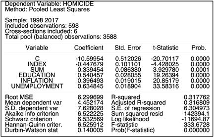
The model received seems to be well built, such as Fisher’s F-statistic suggests. The probability is considerably lower than 0.05, allowing us to reject the null hypothesis of the group means being equal. Unfortunately, this model’s dependent variables explain a rather limited fraction of variance for a dependent variable. According to R2 statistic, the chosen variables explain only 32% of homicides that happened in the 44 countries present in the dataset.

Table 4.1. The outcomes of the Pooled Ordinary Least Squares model

Source: author’s EViews estimations based on Appendix B data.

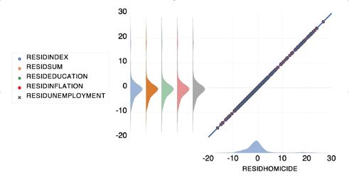
On the other hand, all the variables present in the model are statistically significant at the 1% significance level. In addition, such a situation can also be viewed graphically. Thus, a scatter plot with a regression fit line and Kernel densities illustrates two major statements. The first one concerns Kernel densities of the residuals; an obvious tail is visible towards the positive figure, which is a definite sign of Kurtosis. It means that the distribution of the residuals is unlikely to be normal. Perhaps, the abnormality of the distribution is the result of the presence of extremely crime-ridden states such as Venezuela mentioned in the previous chapter. However, the abnormality is symmetrical and is present for the residuals of all the variables quite similarly. Secondly, the scatter plot represents a very thick distribution of residuals. This may be a sign of a perfect correlation as well as a sign of a biased model, which is to be checked.

Figure 4.1. The POLS model residuals graph

Source: author’s EViews estimations based on Appendix B data.

The model results may be presented in the form of the following equation:

HOMICIDEit = –10.5995414223 – 0.447679179115 × × INDEXit + 0.339453883958 × SUMit + 0.540457315502 × × EDUCATIONit + 0.396493364775 × INFLATIONit + + 0.634844658076 × UNEMPLOYMENTit + εit

(eq. 4.2)

Such a model provides plausible preliminary results. Thus, we can assume that inflation and unemployment have a positive impact on homicide. It is evident from the coefficients that a 1 percentage point change of inflation and unemployment causes a corresponding change in the number of homicides per 100 thousand people, by 0.4 and 0.6, respectively. INDEX, on the other hand, implies the expected effect on homicide; thus, 1 point change in INDEX inversely changes homicide by roughly 0.45.

Nevertheless, Pooled Ordinary Least Squares is not the model of the last resort in this part of empirical findings. OLS models have a tendency to skip specifics of data; thus, Fixed and Random Effects can be used as one of the best fits to the panel type of data.

Even though the Pooled Least Squares model is not a good fit for our data, it can serve as a base ground for choosing between the cross-section effect, the period effect, or their combination. The heteroskedasticity test run on this model can show under which effect assumption should the Fixed and Random

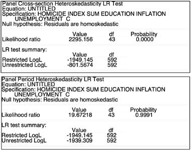
Effects model be run. The theoretical background suggests that a good model has its error term similar along with all the values of the dependent variable. Such a property is called homoskedasticity. The likelihood ratio heteroskedasticity test is run for both cross-section and period. According to the p-values of the tests run, the model’s residuals are homoskedastic under the period assumption (likelihood ratio p-value is 0.9991) and heteroskedastic under cross-section (p-value – 0.0000). Therefore, we may accept the homoskedastic assumption of the effect, namely the period one.

Table 4.2. Cross-section and period effects heteroskedasticity test outcomes

Source: author’s EViews estimations based on Appendix B data.

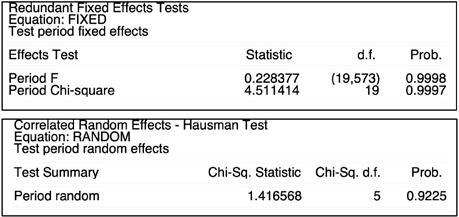
In view of the foregoing, the Fixed Period Effects and Random Period Effects models have to be built and compared for their quality and appropriateness. The comparison criteria are Redundant Fixed Effects – Likelihood Ratio Test and Correlated Random Effects – Hausman Test. They are applied to the Fixed and Random Effects models, respectively. The Redundant Fixed Effects Test’s null hypothesis is that the Fixed Effects model is inappropriate. Based on the test’s probability of both F and Chi-square statistic, we cannot reject the null hypothesis at all levels of significance. At the same time, the Hausman Test has its null hypothesis stating that the Random Effects model is preferred under the given conditions and circumstances. Based on the Chi-square statistic and p-value, it is clear that the null hypothesis cannot be rejected.

Thus, both tests result in null hypotheses not being rejected, i.e. the Random Period Effects model (Panel EGLS) is the most appropriate for the given data.

Table 4.3. Redundant Fixed Effects – Likelihood Ratio Test and Correlated Random Effects – Hausman Test outcomes

Source: author’s EViews estimations based on Appendix B data.

Having decided that the Random Effects is more appropriate, the Pooled OLS model can be declined as a model of lower appropriateness even without Wald’s test. It is known that the Random Effects model approved by the Hausman test revokes the possibility of Pooled OLS being the preferred one (Gujarati & Porter, 2009). Thus, ending up with Period Random Effects is to be used to support or undermine the initial hypothesis of the thesis. The Period Random Effects model takes the form of the following equation:

HOMICIDEit = β0 + β1 × INDEXit + β2 × SUMit + + β3 × EDUCATIONit + β4 × INFLATIONit + + β5 × UNEMPLOYMENTit + εit + [PER = R]

(eq. 4.3)

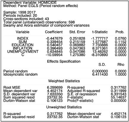
First of all, the model itself must be a significant and reliable one. Thus, a relatively high Fisher’s F-statistic and its low probability value indicate that explanatory variables are significant when explaining the resulting variable, which is a very general indicator of a qualitative model. Independent variables, on the other hand, explain only 32% of the variation of the dependent homicide variable according to the R2 statistic. Another issue of the model that strikes the eye is Durbin-Watson’s first-order serial correlation test. According to its value, the model at hand

suffers from autocorrelation. It is not absolutely unexpected as some of the data used in the model have definite time-related tendencies, which may be the reason for the serial autocorrelation of the model.

Table 4.4. Panel EGLS, Period Random Effect model outcome

Source: author’s EViews estimations based on Appendix B data.

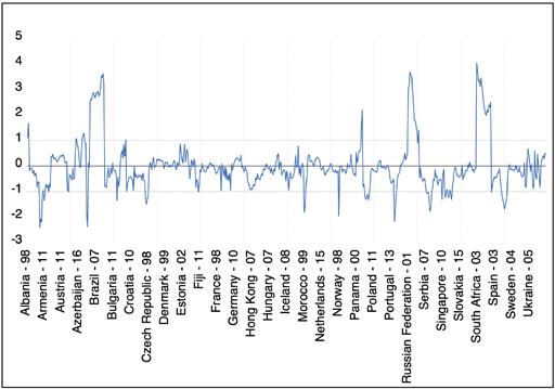
On the bright side, the residuals of the model graphically represented stick to the regression line with a few exceptions. The biggest deviation can be seen in countries such as Brazil, Russia, and South Africa. The effect of chosen independent variables upon the dependent ones may be the least predictable, judging from the high standardized residual values. Apart from that, this residual graph is an indicator of a model with consistent and coherent results sufficient to support the hypothesis.

Figure 4.2. Standardized residual graph

Source: author’s EViews estimations based on Appendix B data.

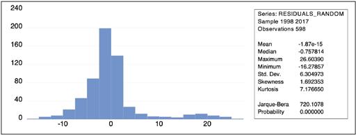
The model’s residuals are also checked for normality and, as it can be seen from the graph, the residuals are not normally distributed. Besides, a huge JarqueBera indicator unambiguously suggests a need to reject the null hypothesis of the normal distribution of residuals. The reasons for the abnormality of the residuals are the same as the reasoning presented for Kernel densities for the Pooled OLS model, countries with severe levels of crime rate cause a tail to the right of the distribution graph. High 7.2 kurtosis only supports the idea and does not allow residuals to draw the expected bell shape of normal distribution.

Figure 4.3. Residuals normality graph

Source: author’s EViews estimations based on Appendix B data.

All in all, the model at hand can be considered an imperfect representation of data used to check the initial hypothesis. However, its quality and significance are altogether sufficient to draw conclusions about the correlation between homicides in individual countries and such factors as legal policies on abortion, education share in government expenditure, inflation, and unemployment. The outcomes of the model are adequate enough to use them as evidence for or against the thesis statement: that free and democratic policy on abortion decreases the level of crime.

Therefore, the variables can now be reviewed. After running the model, its equation with the β parameters is formulated in the following way:

HOMICIDEit = –10.5995414223 – 0.447679179115 × × INDEXit + 0.339453883958 × SUMit + 0.540457315502 × × EDUCATIONit + 0.396493364775 × INFLATIONit + + 0.634844658076 × UNEMPLOYMENTit + εit + [PER = R]

(eq. 4.4)

First of all, the coefficients of the variables are completely the same as they were for the Pooled OLS model; the only differences are t-statistic and probabilities. Thus, it should be noted that all of the variables except SUM (p-value is 0.1192) are statistically significant. Education, inflation, and unemployment are significant at all significance levels (prob. = 0.0000) and INDEX only at the 10% level (prob. = 0.0760). This means that, according to the Random Effects model, similarly as in Pooled OLS, in the case of a change, inflation and unemployment may cause a corresponding change of 0.4 and 0.6 homicides per

100,000 population. The education variable coefficient indicates quite a controversial point; according to it, a 1 per cent change of the education share in government expenditure results in the conforming 0.5 change of the homicide indicator. This is rather unusual as it is commonly believed that education should bring crime down. A particularly plausible explanation might be that education spending comes into effect after students in whose education the government invested have grown up and made their life decision after some years have passed. Such a concept is reviewed and elaborated in the further part of the empirical findings of the thesis.

Having left behind the additional factors affecting the dependent variable, the variables which are essential to this abortion-related research are examined. Thus, for the reasons of imperfection elucidated above, SUM ended up insignificant. Its effect on homicide is rather unreliable as it is hardly a realistic indicator of abortion policies in individual countries. INDEX, on the other hand, is considered significant both theoretically and empirically. A convincing inverse relationship between INDEX and homicide is established. According to the model at hand, a 1 unit change in the INDEX implies an opposite homicide adjustment by almost 0.5 people killed per 100,000 population in a country.

Therefore, this implies that, in addition to the macroeconomic stability being a beneficial asset in crime-fighting process, a diverse elaborated emancipated abortion policy has a relatively strong effect on homicide being a representation of crime. It should also be noted that the effect depicted in this model has its effect based on the mere existence of aforementioned policies permitting abortion, i.e. the effect of any kind of additional policies or procedures simplifying and mainstreaming abortions can have an even greater impact. This particular model also emphasizes the superior importance of actual policies over the policies that only pretend to be so. Such a significant difference between the SUM and INDEX representations of the policies implemented serves as a great example of authentic efficiency of any policy, process, procedure, and other social phenomena. Furthermore, it should be noted that unlike the next part of the research, this model does not account for the actual abortions carried out; it merely discusses an opportunity for women living in the countries observed to make such a decision. The opportunity to act and actual action are very different dimensions, especially in the case of such a controversial matter as abortion, due to cultural and social pressure on a woman’s decision. Thus, it is expected that the number of abortions performed might be an additional driving force bringing the crime rate down. The following part of the research intends to study this question.

4.2 Legal abortions and crime rate trends comparison in the UK

At first, it should be noted that a comparison of historical dynamics and tendencies of the variables of interest, abortions and crime, can show the connection of the variables that can be interpreted in favour or against the initial hypothesis.

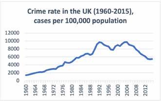
In our case, we can analyse the dynamics of abortion rate and crime rate in the United Kingdom in the period between 1960 and 2015. There are two pieces of data; thus, two charts show the dynamics of changes in the two variables. As it was already mentioned, crime had been continuously growing until the late 1980s, when it suddenly leapt up, peaked, and plummeted. After this, there was one slower increase in the crime rate and a steady decline until the present. The area of interest is the two drops in crime that happened in the UK at the beginning of the 1990s and 2000s. On the other hand, we have abortions which were on a very low level, illegal abortions only, until 1967. This is the year when abortions were legalized in the UK. Starting in 1968, a rapid growth of abortions took place ending six years later, in 1974. This was a period of the enormous growth of abortions performed per 1,000 live births. We can call this period the ‘Abortion Boom’, in an analogy with ‘Baby Boom’ in the USA after the Second World War. Even though abortions peaked in 1974, it should not be considered the end of the ‘Abortion Boom’. It is only logical to put an end to it in the year fluctuations stop, which is circa 1977. After this moment, the abortion rate dynamics became more stable until the end of the 1990s when it grew a little bit more once again and then trailed off.

Now, when we combine the charts, any kind of connection is very difficult to trace if it is there at all. The charts seem to intersect occasionally, but it is definitely not enough to draw any conclusions.

Figure 4.4. Abortion and crime rate dynamics graphs

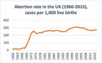
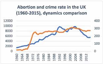
Source: author’s EViews estimations based on Appendix C data.

However, it should not be forgotten that the effect of abortions on crime is delayed. Various researchers have put their effort into studying the question of the age of the most active cohorts of criminals. Thus, the authors of one of the fundamental works in this field, Glaser and Rice, argue that various age groups have various probability or expectancy to commit a crime and end up in jail as their research was based prison data in various parts of the USA. Based on the police and prison reports from 1935 to 1956, the most ‘active’ age group was the ‘25 through 34’ (Glaser & Rice, 1959). ‘21 through 24’ was right behind the leaders. From this, we may conclude that 25–27 is the average age of the most active crime cohorts. Obviously, although the researched time frame is outdated, it is clear that the cultural and social angles of life have changed. Therefore, we can use another work to narrow the age range down. Farrington analysed data from both the USA and UK, comparing three moments in the 20th century:

1938, 1961, and 1983. His result only supports the idea that tendencies in crime change as sharply as any other social economic phenomena. That is why 1983 should be viewed due to its proximity to the period being researched in this thesis. According to Farrington, on average, the most arrested age group in the USA in 1983 was 28.4-year-old people, while in the UK, this group was 24.9-yearold ones (1986). He also discussed the peak of arrests for both countries: they were 18 years old age of arrested for Americans and 15 – for British. It can be concluded that the British used to begin and thrive in their criminal career a few years earlier than their American peers. At last, it seems wise to refer to more modern research focused mainly on Britain, the field of interest of this thesis. In her work, Hansen has studied the age profiles for various types of crime among young people of two groups, with a higher and lower level of education. Even though she claims that the more educated have a higher probability of stepping away from crime by the age of 25, while the less educated do not show this kind of tendency, she states that the age around 25 is a threshold for crime (Hansen, 2003). This is the age of transition from low- or non-violent crime to socially abusive violent crime.

Based on the research papers by Glaser & Rice and Farrington as well as Hansen, we may approximately assume that the delay between an abortion and its effect is 25 years for theoretical purposes. Under this assumption, some modifications should be applied to the chart of the abortion and crime rate in the UK dynamics. As the effect is delayed by 25 years, then its graphical representation should be a chart shifted by the same number of years. As it can be interpreted that the abortions done in 1969 will affect the crime rate only in 25 years, in 1994, thus the 1969 abortion value corresponds to the 1994 crime value graphically. The perpendicular dotted lines represent the peaks mentioned and explained above; these peaks are followed by downslides of crime. These particular points are the reference points of interest for the work done in this thesis as they represent the most illustrative examples of a possible correlation between abortion and crime.

The graph below shows that the beginning of the ‘Abortion Boom’ perfectly fits the moment when the crime plummeted in 1992 under the assumption of 25 year abortion delay being effective. The year when abortions were legalized, 1967, is clearly in line with the crime drop, which happened 25 years later. The end of ‘Abortion Boom’ in 1977 described above, however, did not correspond to the second drop in crime in 2004 so perfectly, its effects preceded the drop by two years. Nevertheless, the comparison of the dynamics suggests the existence of a very vague, not yet elaborated connection between the variables of interest over time in the long run.

Figure 4.5. Abortion and crime rate dynamics graph, delayed

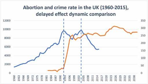
Source: author’s EViews estimations based on Appendix C data.

All in all, the comparison of the trends is a great illustration of a possible correlation between the abortion rate and crime rate in the UK. It quite vividly shows how the two significant periods for indicators fit each other, suggesting the existence of a connection. Nevertheless, it may not be enough to provide evidence in favour or against the initial hypothesis. Thus, more sophisticated approaches should be applied to the data at hand.

4.3 The UK study of the legal abortions effect on crime rate analysis

The second major approach to empirical research of the initial hypothesis is mainly concerned with the country-level scale and more specific data dimensions. In this part, the case of the UK is reviewed in the period between 1960 and 2015. This model is used to study the effect of actual abortions performed on the crime rate as an extension of the previous part.

Thus, as the research’s outline is set and analysed in the preceding chapter, the model has to have a few distinct features. The major feature of the model is the delayed effect of some variables taken into account. Thus, it is believed that both the abortion rate and the government expenditure on

education variables are expected to carry out their effect upon the crime rate of the UK. The deferred effect of abortions is already a determined matter as, according to the studies reviewed above, the age of the highest activeness of crime elements is 25 years in the UK. From this, we may draw a conclusion that the effect of abortion, i.e. the absence of birth of a potential criminal is deferred for around 25 years. However, the matters with education delay are yet unclear.

Both abortions and education deferred period are to be defined with experiments with the data. The essence of the experiments lies in trying out variously delayed abortion and education variables combined with other variables present in the model in order to find out the combination that falls into the logically determined range and is statistically significant. The experiments are to be run on the basis of a simple Ordinary Least Squares model as it proves to be enough to trace some correlations between variables. The assumptions are applied when experimenting indicates that the delay for abortions’ effect lies around the period of 25 years, while the delay for education should correspond to the following logical assumption:

Ded = Dab – Asc (form. 4.1)

This logical assumption means that the education effect delay equals the difference between abortion effect delay, which also stands for the age of the highest criminal activity, minus the age of an average British school student when deliberate significant education begins. In the UK, Asc, the age of beginning more serious study, corresponds with the Key Stage 3 (secondary school) of ‘National Curriculum for England’, a school system implemented by the government by the Education Reform Act of 1988 (GOV.UK 2020). According to it, this age is approximately 12–14 years. It is also the age that is called transitional or litigious age, one of the most important periods in any person’s life due to the great physical and mental changes of a person which are extremely important for future determination and destiny definition.

Thus, a set of experimental models produces an outcome of 24-year abortion effect delay and 11-year educational delay. This means that an abortion carried out affects the level of crime after 24 years from the moment when it was performed, as the abortion results in an unwanted child potentially not committing a crime at the age most appropriate for that crime. The results also illustrate that the quality of education received during teenage years, the age of around 13 years, makes a great deal of life decision impact for a person, potentially changing the life path of a person in education. Such results fall into

the theoretical and logical ranges, meaning that they can and should be used in the research.

Now, with the delays used in the theoretically and experimentally agreed model, the models estimating the variables and their effect on the dependent variable should be built and reviewed. The first step in the process of checking the initial hypothesis that abortions negatively affect crime is Newey-West Ordinary Least Squares. This variation of the OLS model provides more robust results than the regular variation of the OLS model. However, as previously, such a model is run mainly to see the vague results of the regression with the variables at hand. Thus, the model equation has the following form:

CRIME_RATEt = β0 + β1 × ABORTIONt-25 + + β2 × EDUCATIONt-13 + β3 × INFLATIONt + + β4 × UNEMPLOYMENTt + εt

(eq. 4.5)

The model built is of a significant nature, which is known due to low F-statistic probabilities, both Fisher and Wald, a high R2 value; also, Akaike info, Schwarz, and Hannan-Quinn criteria are high. On the other hand, the Durbin-Watson statistic indicator suggests the first order serial correlation present in the model, which will be dealt with later on.

Table 4.5. The outcomes of the Newey-West Ordinary Least Squares model

Source: author’s EViews estimations based on Appendix C data.

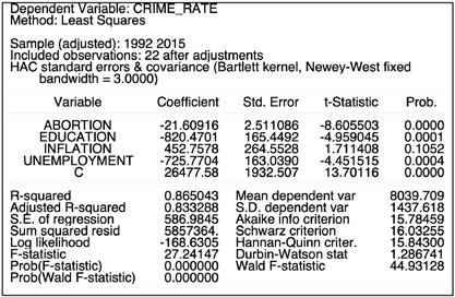
The robust nature of the model means that the residuals are normally distributed, and the model is homoskedastic; the model is also stable in accordance with the Ramsey RESET Test. The standardized residual graphical representation also suggests the robustness of the model.

Figure 4.6. The Newey-West Ordinary Least Squares model residuals graph and residuals distribution normality

Source: author’s EViews estimations based on Appendix C data.

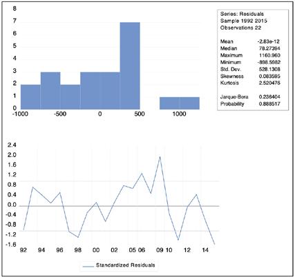
The variables themselves are significant as well, all of them but one are significant at 1% significance, and inflation is only marginally significant at the 10% level. The abortion, education, and inflation variables show a logically acceptable result in the form of the coefficients. Thus, inflation is positively correlated with the crime rate with the β parameter of 452.8, while education and abortions negatively correlate with the crime rate: 1 unit change in either of them leads to an inverse change of 820.5 and 21.6 units in the crime rate, respectively. All in all, the substituted coefficients of the model look as follows:

CRIME_RATEt = 26477.5779364 – 21.6091569257 × × ABORTIONt – 820.470050312 × EDUCATIONt + + 452.757808873 × INFLATIONt – 725.770410334 × × UNEMPLOYMENTt + εt

(eq. 4.6)

However, there are better uses of the data provided. The previously described cointegration phenomenon is a great approach to be applied to the data to see if the dependent and independent variables have any long-term relationships.

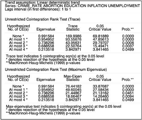
First, the Johansen Cointegration Test is applied to the data we have under 1 to 1 lag interval condition to check the long-term presence correlation between the variables. The test uses two methods, Trace and Maximum Eigenvalue, to check if cointegrating equations are present. The results received are similar for both methods, so they can be treated equally.

Table 4.6. The Johansen Cointegration Test outcome

Source: author’s EViews estimations based on Appendix C data.

Thus, based on the results of both methods, none and at most 1 through 4 equation options can be rejected at the 5% significance level, i.e. both tests indicate five cointegrating equations at 5% significance level. This is a strong suggestion that a long term relationship exists between the variables.

It is also possible to examine the equation under the Johansen Cointegration Test assumption, i.e. the normalized cointegrating equation. First of all, a high t-statistic for all of the variables allows us to reject the null hypothesis of no cointegration. Before the coefficients are reviewed, it should be noted that in the case of long-term relationships in the Johansen Cointegration Test, the coefficients are reversed. Thus, we can see that unemployment, surprisingly, is still negative as in the Newey-West OLS, suggesting that changes in unemployment result in an inverse change in the crime rate in the UK. The variable of interest, abortion has a coefficient of 26, i.e. every unit change of abortions per 1,000 live births results in an inverse reaction of the crime rate by 26 units.

Table 4.7. The Johansen Cointegration Test coefficient

Source: author’s EViews estimations based on Appendix C data.

The next step of the estimation of given data is the Cointegration model with the Fully-Modified OLS method applied. However, in order to do it, the stationarity of the variables needs to be examined. Thus, every variable needs to be checked for a unit root test, including only intercept testing and with the automated lag selection according to the Akaike Info Criterion. Based on this, the following results were drawn. Inflation is the only stationary variable at level; all others are stationary at first difference but one. There is an issue with the education variable; it is not stationary at any level because of a rather small number of observations; however, it was decided to keep it for the sake of the model’s integrity and to treat it as stationary at level as the Augmented Dickey-Fuller test statistic is the closest to the threshold allowing the rejection of the null hypothesis of a unit root. This variable, however, should be treated more cautiously in the model. All in all, the Cointegration model is to be built with education and inflation at level and the crime rate, abortion, and unemployment at first difference modification.

Variable ADF Prob.

CRIME_RATE

ABORTION

EDUCATION

INFLATION

UNEMPLOYMENT

Table 4.8. Unit root tests outcome

At level 1st difference 2nd difference Stationary at

0.4158 0.0011 0.0007 1st difference

0.4522 0.1030 0.0000 1st difference

0.1954 0.9089 – level*

0.0057 0.0009 0.0029 level

0.3000 0.0041 0.002 1st difference

Source: author’s EViews estimations based on Appendix C data.

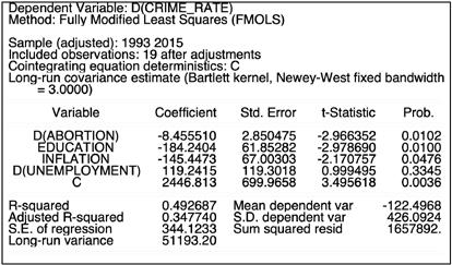
The Fully modified OLS Cointegration model with stationary variables built with the Barlett Kernel option and the Newey-West bandwidth method results in the model formed using the following equation:

D(CRIME_RATE)t = β0 + β1 × D(ABORTION)t + + β2 × EDUCATIONt + β3 × INFLATIONt + + β4 × D(UNEMPLOYMENT)t + εt

(eq. 4.7)

The model should satisfy the requirement put before it. It explains almost 50% of the crime rate variance, according to R2, meaning that there are other factors not included that also have their effect upon the crime rate. Unlike previous methods applied to the data, FMOLS results suggest that unemployment is insignificant as its t-statistic is 0.99, too low for a significant variable.

Table 4.9. The FMOLS Cointegration model outcome

Source: author’s EViews estimations based on Appendix C data.

The quality of the model check with the Engle-Granger Cointegration test may also be applied. The results received clearly suggest that there is no cointegration between variables; thus, no long-term relations are noted. However, it is commonly known that the Engle-Granger test is not reliable when working with multiple variables, unlike the Johansen Cointegration Test. Thus, its results are not to be trusted.

On the other hand, the Engle-Granger works perfectly well with only two variables, in this case, the crime rate and abortions. The Engle-Granger applied to only those variables suggests results in the Engle-Granger z-statistic value of –14.67677 and probability of 0.1002, which is marginally significant at the 10% significance level. In addition, the differenced residual value in the Engle-Granger Test is significant as well, now at the 1% significance level. From this, the conclusions may be drawn that in accordance with the Engle-Granger Cointegration Test, the abortion and crime rate variables are significantly cointegrated, i.e. related in a long run. Thus, the result of FMOLS Cointegration model may be trusted at least concerning the abortion and crime rate relation checked by the test.

Table 4.10. The Engle-Granger outcome for the abortion and crime variables

Source: author’s EViews estimations based on Appendix C data.

Thus, reviewing the coefficients resulting from the FMOLS, we may observe leaving unemployment behind due to its insignificance, that the inflation variable presents an issue similar to the one which happened to unemployment during the Johansen Cointegration Test and Newey-West OLS, the coefficient defies common sense. The relation between inflation and crime is negative, meaning that changes in inflation lead to inverse changes in the crime rate. Particularly, an increase in inflation by 1% would mean a decrease in the crime rate by 145 crime cases per 100,000 population. Such an unusual situation may only be explained by the long-term nature of the coefficient. Thus, it is obvious that in a short run, inflation reduces the purchasing power of consumers, leaving the demands and

wishes on the same level easily fulfilled by cheap stolen products provided by the crime world, which only encourages the latter to act (Rosenfeld, 2014). However, in the long run, such a relation may be mitigated and even reversed. Government spending on education has an inverse long-term relation to the crime rate, too. According to FMOLS, a 1% change results in 184-unit inverse change in the crime rate. Such results fall into any kind of a common-sense or theoretical explanation possible. Nevertheless, the variable of interest is abortion, and its coefficient is –8.5, which clearly suggests a negative relationship in the long run between this variable and the dependent variable. It is expected that with every abortion carried out per 1,000 live births, the crime rate decreases by 8.5 cases per 100,000 population.

Table 4.11. The FMOLS Cointegration model coefficients

Source: author’s EViews estimations based on Appendix C data.

Such results may also be presented in the following form of substituted coefficients:

D(CRIME_RATE)t = 2446.81348292 – – 8.45551042959 × D(ABORTION)t – 184.240405884 × × EDUCATIONt – 145.447311792 × INFLATIONt + + 119.241497526 × D(UNEMPLOYMENT)t + εt

(eq. 4.8)

Compared to that of education, the abortion coefficient may seem not large and serious enough to be considered. However, this is an illusion of scale and depth. Thus, in a recent illustrative year, 2015, only 273.7 abortions took place for every 1,000 live births, of which there were 731,217. From this, we may estimate that abortions performed during 2015 will reduce the crime level of the year 2039 , 24 years from 2015, by roughly 1.7 million cases of crime activities reported. For reference, in 2015, there were about 3.5 million crime cases in total in the UK.

The preceding findings suggest the number of legal abortions that can affect the crime rate. Besides, when coefficients retrieved from the Johansen

Cointegration Test are applied to similar estimations, the decrease in crime cases by 1.7 million in 2039 due to abortions carried out in 2015 changes to an incredible 5.2 million.

Therefore, from this model, we have received results stating that the longterm correlation between legal abortion and the crime rate actually exists. During the course of action, various methods were applied to reach such a conclusion; however, the Johansen Cointegration Test and the Fully Modified Ordinary Least Squares model are most compelling. Thereby, according to the first one, the change in the number of abortions per 1,000 live births by one unit corresponds to about 26-unit reverse change in the crime rate (cases of all crime activity per 100,000 population), while the second one suggests that the coefficient of the correlation is only 8.5. Hence, as FMOLS is considered more trustworthy out of the two, the final coefficient is decided upon as a weighted average, when the weights are given due to the author’s own estimation (Gujarati & Porter, 2009). Thus, an assumption of FMOLS weighing 65% of the final abortion-to-crime correlation coefficient, and Johansen Cointegration Test weighing 35% seems to be justified by common experience of the combined usage of the aforementioned econometric methods. From this, we can easily assume that the effect of the abortion coefficient on the crime rate is roughly 15.

Such findings correspond to and complement the findings from part one of the research. It is clear from the econometric discoveries that actual abortions influence the crime rate as does the legal background that lies behind abortion policies and procedures. Altogether, we can draw a conclusion that the initial hypothesis of the thesis cannot be rejected in two dimensions, legal, concerning legal abortion-related policies, and actual, concerning the actual abortions that women undergo. It is also important to understand that abortion policies, as well as abortions performed, are expected to come into effect and influence the crime rate after the passage of time required by potential demoralised children to become criminals.

4.4 Discussion of the received results

To conclude, there are three approaches used in the empirical part of the research to support or undermine the null hypothesis that legal abortion has a strong significant negative effect on the crime rate. The three approaches are the Period Random Effects model built on the basis of panel data of countries with data on the legal status and policies concerning abortions and homicide in 44 countries over a period of 20 years, a general comparison of dynamics of

crime rate, i.e. total crime number per 100,000 from 1960 to 2015 and delayed dynamics of abortions carried out in the UK during the same period, and the Fully Modified OLS model with the previously mentioned data on the number of abortions and the crime rate in the UK. Even though the final purpose of the methods is the same, not only the methods but also dimensions of research applied are different.

Thus, the Period Random Effects model applied to panel data studies the effect of the legal grounds for abortion in countries of the world. In particular, there are nine legal grounds accepted worldwide, allowing a woman to undergo an abortion; there is also a measure of the latest term of gestation until which the abortion is legal. An estimator based on the two factors mentioned is the representation of the level of freedom of the abortion policy in any given country. Hence, with the econometric methods applied, it is concluded that the legal background allowing for abortions may have a potent effect on crime. Thus, if a country is fully legalizing one of nine legal grounds for abortions with a maximum gestational limit or two legal grounds with half a maximum gestational limits, three grounds with one-third of maximum gestational limit each, or finally any other combination of the number of legalized abortion grounds and gestational limit producing 1 according to the aforementioned INDEX formula, the country may expect a homicide drop by somewhere around 0.5 homicides per 100,000 population. For reference, the average homicide level for the world is only 5.3 and this is mainly due to some states having monstrous levels of crime; other countries, such as Poland in 2017, recorded only 0.8 homicides per 100,000 population. For such states, the implementation of such policies would mean a world of difference. There is no doubt in saying that a –0.5 change in the homicide rate due to a one unit change of the INDEX is merely an approximation of the averaged global effect represented by 44 countries. Thus, countries with an already low homicide rate or very strong cultural or social pressure on abortion-related decisions would not be expected to benefit so strongly from changes in legal abortion statuses. However, legal grounds and the gestational limit are only the tips of policies influencing the real availability of abortions in individual countries, especially for the latter types of countries. Hereby, in countries with strong cultural and social animadversion, the gestational limit regulations are not the major reason for abortions not being a matter of free choice. Apart from social judgement and disapproval, other ways to restrain women’s freedom to have abortions exist, some of them even enshrined in law. For instance, there are countries where a woman who has undergone an abortion is supervised by police or other law enforcement institutions like a common criminal, in other countries, abortions are impossible without spousal consent;

there are even places on the Earth where sex restrictions are applied to abortions meaning that abortions can only be carried out if the foetus is confirmed to be of a particular sex, usually female foetuses are allowed to be aborted while male ones are not. These and other factors of withholding women’s right to undergo abortions if they wish to do so, together with the absence of legal grounds for abortions and low gestational limits may be, and most likely are, the reasons for children with a higher risk of committing a crime being born. It should be reminded that unwanted children or pregnancies that can potentially result in abortion, if it is allowed, have a much higher chance to deviate and choose the path of crime due to reasons such as being traumatized by not receiving enough parenting love, lack of discipline, low standards of living, negative influence of the surroundings, and other. Thus, from the theoretical reasoning and empirical evidence, we may draw a conclusion that high freedom in the legal status of abortion promoted by appropriate policies and social changes towards freedom of choice may be of much use to decrease crime.

On the other hand, we have some evidence in favour of the initial hypothesis presented with the help of the time series from the UK. This data provides another point of view, different from the previous one as it does not look at the legal ability to undergo abortions, but reviews actual abortions carried out in the UK in the period from 1960 to 2015 and their effect on the crime rate some years after they were performed. The first piece of evidence available with this data is a mere comparison of the dynamics of the variables of interest, abortion and crime rate. As there are two peaks followed by downslides in the crime rate, there is also a period we call the ‘Abortion Boom’ in the UK between 1968 and 1977, which fits almost perfectly into the graphic representation of crime. We observe the first drop of the crime rate 25 years after the beginning of the ‘Abortion Boom’ and another one about 27 years after its end. It is a piece of rather simple but imposing evidence in favour of abortion being negatively correlated to crime. Nevertheless, the Fully Modified OLS Cointegration model has also been applied to the data at hand, together with the Johansen and Engle-Granger Cointegration Tests. All of them strongly suggest that there is a longterm relationship between the abortion and the crime variable. The model and tests also result in an estimated coefficient stating that every abortion conducted per 1,000 live births in the UK, on average, results in around 15 crime cases fewer per 100,000 population after 24 years. It has been elaborated before that even such a small coefficient with modern levels of the abortion rate in the UK has a great impact on lowering the crime rate in the long run. Yet, it is should be obvious that such results may not necessarily be similar in other countries or regions due to the difference of exogenous factors present. Nevertheless, it is

clear that not only the legal status of abortions matters but also their actual number. The number may in fact be a representation of the legal policies being implemented in real life. The United Kingdom may actually be considered a country with an average, considerable level of freedom as regards the abortion policies. The cultural and social attitude towards abortions is quite positive too. Together, this leads to considerable abortion rates. Thus, the factual abortion rate variable represents the effect of social and cultural burden not present in the legal grounds-related part of the research filling the gaps in the explanation of the crime rate variance. This gives us grounds to confirm the statement that the legalization of abortion may result in a considerable crime rate reduction and provide additional evidence in favour of the statement that processes of judicial, social, and cultural nature have great importance, too. Therefore, these findings are yet another piece of evidence in favour of the hypothesis that legal abortions are a significant tool in fighting crime in the way of reducing the number of unwanted, unloved children, or children born and raised in inappropriate conditions, who have high chances of becoming criminals.

To conclude, the methodology used in this work proves to be useful in supporting the statement that legal abortions have a strong effect on the crime rate. The matter is reviewed from two points of view: legal policies concerning abortion implemented in individual countries and actual abortions performed as a result of the aforementioned policies. The results of both approaches may be briefly summarised in an interpretation stating that the legalization of abortions can be quite beneficial for a country in terms of fighting crime by allowing people freedom to decide not to have unwanted children who could potentially have higher chances of becoming criminals.