Buy ebook Basic transesophageal and critical care ultrasound first edition couture cheap price by Ebook Home

Basic Transesophageal and

Care Ultrasound First Edition Couture

Visit to download the full and correct content document: https://textbookfull.com/product/basic-transesophageal-and-critical-care-ultrasound-fir st-edition-couture/

More products digital (pdf, epub, mobi) instant download maybe you interests ...

100 Cases in Emergency Medicine and Critical Care, First Edition Mistry

https://textbookfull.com/product/100-cases-in-emergency-medicineand-critical-care-first-edition-mistry/

Point of Care Ultrasound 2nd Edition Nilam Soni

https://textbookfull.com/product/point-of-care-ultrasound-2ndedition-nilam-soni/

Critical Care of Children with Heart Disease : Basic Medical and Surgical Concepts Ricardo A. Munoz

https://textbookfull.com/product/critical-care-of-children-withheart-disease-basic-medical-and-surgical-concepts-ricardo-amunoz/

Pastoral theology and care : critical trajectories in theory and practice First Edition Ramsay

https://textbookfull.com/product/pastoral-theology-and-carecritical-trajectories-in-theory-and-practice-first-editionramsay/

Point of Care Ultrasound Made Easy John Mccafferty

https://textbookfull.com/product/point-of-care-ultrasound-madeeasy-john-mccafferty/

Nursing in Critical Care Setting: An Overview from Basic to Sensitive Outcomes Irene Comisso Et Al.

https://textbookfull.com/product/nursing-in-critical-caresetting-an-overview-from-basic-to-sensitive-outcomes-irenecomisso-et-al/

Practical Point-of-Care Medical Ultrasound 1st Edition

James M. Daniels

https://textbookfull.com/product/practical-point-of-care-medicalultrasound-1st-edition-james-m-daniels/

Point of Care Ultrasound Made Easy 1st Edition John Mccafferty (Editor)

https://textbookfull.com/product/point-of-care-ultrasound-madeeasy-1st-edition-john-mccafferty-editor/

Lange Critical Care John M. Oropello

https://textbookfull.com/product/lange-critical-care-john-moropello/

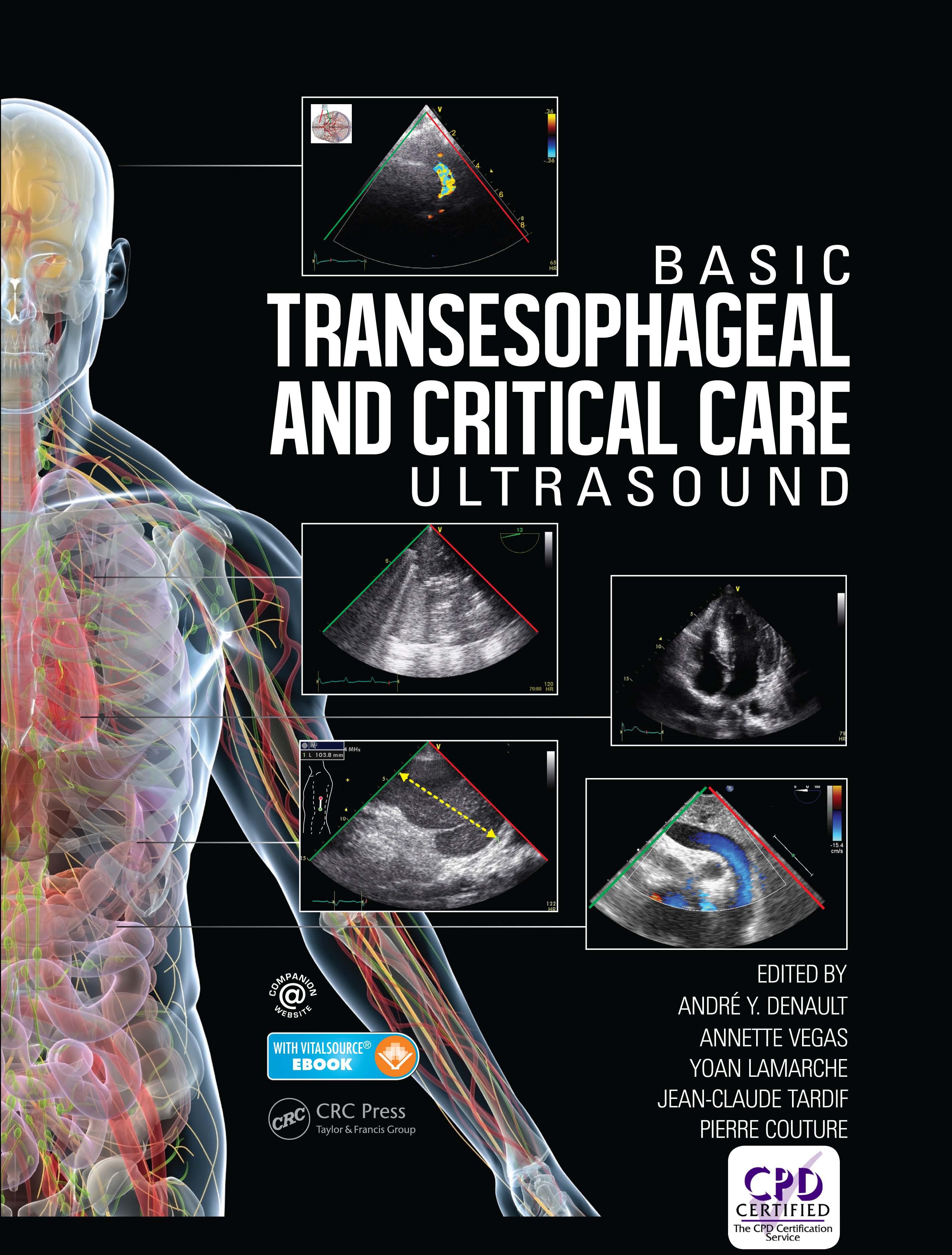
In stitut de C ar dio logie de Montréal , Qu é bec, Canada

To ronto General Hospital Ontario, Canada

In stit ut de C a rdiolo gie de Montr éa l and H ôpita l du Sacré-Coeur de Montré al , Québec, C anada

Rese a rch Center at th e Montr eal He a rt Ins t itut e , Québe c , C anada

In stitut de C a rdio l ogi e d e Montré al , Qu éb ec, C anada

CRC Press

Taylor & Francis Group

6000 Broken Sound Parkway NW, Suite 300

Boca Raton, FL 33487-2742

CRC Press is an imprint of Taylor & Francis Group, an Informa business

No claim to original U.S. Government works

Printed on acid-free paper

International Standard Book Number-13: 978-1-4822-3712-2 (Pack – Book + eBook)

This book contains information obtained from authentic and highly regarded sources. While all reasonable efforts have been made to publish reliable data and information, neither the author[s] nor the publisher can accept any legal responsibility or liability for any errors or omissions that may be made. The publishers wish to make clear that any views or opinions expressed in this book by individual editors, authors or contributors are personal to them and do not necessarily reflect the views/opinions of the publishers. The information or guidance contained in this book is intended for use by medical, scientific or health-care professionals and is provided strictly as a supplement to the medical or other professional’s own judgement, their knowledge of the patient’s medical history, relevant manufacturer’s instructions and the appropriate best practice guidelines. Because of the rapid advances in medical science, any information or advice on dosages, procedures or diagnoses should be independently verified. The reader is strongly urged to consult the relevant national drug formulary and the drug companies’ and device or material manufacturers’ printed instructions, and their websites, before administering or utilizing any of the drugs, devices or materials mentioned in this book. This book does not indicate whether a particular treatment is appropriate or suitable for a particular individual. Ultimately it is the sole responsibility of the medical professional to make his or her own professional judgements, so as to advise and treat patients appropriately. The authors and publishers have also attempted to trace the copyright holders of all material reproduced in this publication and apologize to copyright holders if permission to publish in this form has not been obtained. If any copyright material has not been acknowledged please write and let us know so we may rectify in any future reprint.

Except as permitted under U.S. Copyright Law, no part of this book may be reprinted, reproduced, transmitted, or utilized in any form by any electronic, mechanical, or other means, now known or hereafter invented, including photocopying, microfilming, and recording, or in any information storage or retrieval system, without written permission from the publishers.

For permission to photocopy or use material electronically from this work, please access www.copyright.com (http://www. copyright.com/) or contact the Copyright Clearance Center, Inc. (CCC), 222 Rosewood Drive, Danvers, MA 01923, 978-750-8400. CCC is a not-for-profit organization that provides licenses and registration for a variety of users. For organizations that have been granted a photocopy license by the CCC, a separate system of payment has been arranged.

Product or corporate names may be trademarks or registered trademarks, and are used only for identification and explanation without intent to infringe.

Visit the Taylor & Francis Web site at http://www.taylorandfrancis.com and the CRC Press Web site at http://www.crcpress.com

Visit Companion Website: www.crcpress.com/cw/denault

Dedication

This book is dedicated to:

My wife Denise Fréchette and my children Jean-Simon, Gabrielle, and Julien who have supported me with love and patience (André Y Denault)

My parents, Patrick and Lena, and my brother Derek, who have always been supportive (Annette Vegas)

Maude and Julien for their support and inspiration (Yoan Lamarche)

Michèle, Jean-Daniel and Pier-Luc (Jean-Claude Tardif)

Frédéric and Noémie (Pierre Couture)

And above all, our patients for whom we believe that knowledge in the use of bedside ultrasound will improve their care.

The editors would like to thank sincerely Dora and Avrum Morrow and the Richard I Kaufman Endowment Fund in Anesthesia and Critical Care.

Avrum Morrow

Richard I Kaufman

List of contributors

Martin Albert, MD, FRCPC Associate Professor of Medicine, Internist and Intensivist, Department of Medicine and Critical Care, Hôpital du Sacré-Coeur de Montréal Research Center and Intensivist, Department of Surgery, Institut de Cardiologie de Montréal, Université de Montréal, Montréal, Québec, Canada

Christian Ayoub, MD, B.Pharm, FRCPC Clinical Assistant Professor, Department of Cardiac Anesthesiology, Institut de Cardiologie de Montréal, Department of Anesthesiology, Maisonneuve-Rosemont Hospital, Université de Montréal, Montréal, Québec, Canada

Mustapha Belaidi, MD Department of Cardiac Anesthesiology, Centre Hospitalier Universitaire (CHU) de Nantes, Nantes, France

François M. Carrier, MD, FRCPC Clinical Assistant Professor, Department of Anesthesiology and Division of Critical Care, Department of Medicine, Centre Hospitalier de l’Université de Montréal (CHUM), Université de Montréal, Montréal, Québec, Canada

D. Catalina Casas Lopez, MD Department of Anesthesia and Perioperative Medicine, London Health Sciences and St. Joseph’s Health Care, University of Western Ontario, London, Ontario, Canada

Yiorgos Alexandros Cavayas, MD, FRCPC Critical Care Fellow, Université de Montréal, Montréal, Québec, Canada

David-Olivier Chagnon, MD, FRCPC Department of Radiology, Hôpital Pierre-Boucher, Longueuil, Québec, Canada

Carl Chartrand-Lefebvre, MD, FRCPC Clinical Professor, Department of Radiology, Centre Hospitalier de l’Université de Montréal (CHUM), Université de Montréal, Montréal, Québec, Canada

Robert Chen, MD, FRCPC Assistant Professor of Anesthesia, Cardiac Anesthesia and Intensive Care, University of Ottawa Heart Institute, University of Ottawa, Ottawa, Ontario, Canada

Anne S. Chin, MD, FRCPC Assistant Professor, Department of Radiology, Cardiothoracic Section, Centre Hospitalier de l’Université de Montréal (CHUM), Université de Montréal, Montréal, Québec, Canada

Jennifer Cogan, MD, M.Epid, FRCPC Associate Professor, Department of Anesthesiology, Institut de Cardiologie de Montréal, Université de Montréal, Montréal, Québec, Canada

Geneviève Côté, MD, MSc, FRCPC Assistant Professor, Pediatric Cardiac Anesthesiologist, Department of Pediatric Anesthesia, Centre Hospitalier Universitaire (CHU) Mère-Enfant SainteJustine, Université de Montréal, Montréal, Québec, Canada

Pierre Couture, MD, FRCPC Clinical Associate Professor, Cardiac Anesthesiology Department, Institut de Cardiologie de Montréal, Department of Anesthesiology, Université de Montréal, Montréal, Québec, Canada

André Y. Denault, MD, PhD, FRCPC, FASE, ABIM-CCM, FCCS Professor, Critical Care Ultrasound Training Program Director, Department of Cardiac Anesthesiology and Division of Critical Care of the Department of Cardiac Surgery, Institut de Cardiologie de Montréal and Division of Critical Care of the Department of Medicine, Centre Hospitalier de l’Université de Montréal (CHUM), Université de Montréal, Montréal, Québec, Canada

Georges Desjardins, MD, FRCPC, FASE Associate Professor of Anesthesiology, Director of Perioperative Echocardiography, Department of Anesthesiology, Institut de Cardiologie de Montréal,Université de Montréal, Montréal, Québec, Canada

Vinay K. Dhingra, MD, FRCPC Clinical Associate Professor of Medicine, Medical Director Quality Critical Care Vancouver Acute Clinical Lead, Department of Medicine, Division of Critical Care, Vancouver General Hospital, University of British Columbia, Vancouver, British Columbia, Canada

Jean-Nicolas Dubé, MD, MA, FRCPC Clinicial Instructor, Department of Internal Medicine, Division of Critical Care, Centre intégré universitaire de santé et de services sociaux de la Mauricie-et-du-Centre-du-Québec, Université de Montréal, TroisRivières, Québec, Canada

Ashraf Fayad, MD, MSc, FRCPC, FCARCSI, FACC, FASE Associate Professor, Director of Perioperative Hemodynamic Echocardiography, Department of Anesthesiology, University of Ottawa, Ottawa, Ontario, Canada

Gordon N. Finlayson, BSc, MD, FRCPC (Anesth and CCM) Clinical Assistant Professor, Division of Critical Care, Department of Anesthesiology and Perioperative Care, Vancouver General Hospital, University of British Columbia, Vancouver, British Columbia, Canada

Annie Giard, MD, FRCPC Emergency Room Physician, Responsible for Echography Training in Emergency Medicine and Family Medicine, Université de Montréal, ARDMS, Local Manager for the Training of Independent Practitioner of CEUS, Department of Emergency Medicine, CIUSS du Nordde-l’Îlede-Montréal, Installation Hôpital du Sacré-Coeur de Montréal, Montréal, Québec, Canada

Martin Girard, MD, FRCPC Clinical Associate Professor, Department of Anesthesiology, Division of Critical Care of the Department of Medicine, Centre Hospitalier de l’Université de Montréal (CHUM), Université de Montréal, Montréal, Québec, Canada

Donald E.G. Griesdale, MD, MPH, FRCPC Assistant Professor, Department of Anesthesiology, Pharmacology and Therapeutics, Department of Medicine, Division of Critical Care Medicine, Chair, Vancouver Medical Advisory Council, Vancouver General Hospital, University of British Columbia, Vancouver, British Columbia, Canada

Han Kim, MD, FRCPC Assistant Professor, Department of Anesthesia, St. Michael’s Hospital, University of Toronto, Toronto, Ontario, Canada

Manoj M. Lalu, MD, PhD, FRCPC Clinical Scholar, Department of Anesthesiology, The Ottawa Hospital, Regenerative Medicine Program, The Ottawa Hospital Research Institute, Ottawa, Ontario, Canada

Yoan Lamarche, MD, MSc, FRCSC Assistant Professor of Surgery, Cardiac Surgeon and Intensivist, Department of Cardiac Surgery, Institut de Cardiologie de Montréal and Hôpital du Sacré-Coeur de Montréal, Université de Montréal, Montréal, Québec, Canada

Moishe Liberman, MD, PhD Associate Professor of Surgery, Director, CHUM Endoscopic in Tracheobronchial and Oesophageal Center (C.E.T.O.C.), Marcel and Rolande Gosselin Chair in Thoracic Surgical Oncology, Scientist, Research Center, Centre Hospitalier de l’Université de Montréal (CHUM), Université de Montréal, Montréal, Québec, Canada

Feroze Mahmood, MD, FASE Associate Professor of Anesthesia, Harvard Medical School, Director Vascular Anesthesia and Perioperative Echocardiography, Beth Israel Deaconess Medical Center, Boston, U.S.A.

Ramamani Mariappan, DA, MD, Dip.NB Professor, Christian Medical College, Vellore, India

Serge McNicoll, MD, CSPQ Cardiologist, Chief of Cardiology Department of the Department of Medicine, Hôpital Régional de St-Jérôme, Université de Montréal, Montréal, Québec, Canada

Massimiliano Meineri, MD Associate Professor of Anesthesia, Staff Anesthesiologist, Director Perioperative Echocardiography, Toronto General Hospital, University of Toronto, Toronto, Ontario, Canada

Scott J. Millington, MD, FRCPC Assistant Professor, Department of Critical Care Medicine, The Ottawa Hospital, University of Ottawa, Ottawa, Ontario, Canada

Blandine Mondésert, MD Assistant Professor, Cardiologist, Division of Cardiac Electrophysiology, Department of Medicine, Adult Congenital Heart Disease Center, Institut de Cardiologie de Montréal, Université de Montréal, Montréal, Québec, Canada

Céline Odier, MD, FRCPC Assistant Clinical Professor, Department of Neurosciences, Centre Hospitalier de l’Université de Montréal (CHUM), Université de Montréal, Montréal, Québec, Canada

Sarto C. Paquin, MD, FRCPC Assistant Professor, Department of Medicine, Division of Gastroenterology, Centre Hospitalier de l’Université de Montréal (CHUM), Université de Montréal, Montréal, Québec, Canada

Eric Piette, MD, MSc, FRCPC Clinical Assistant Professor, Emergency Room Physician, Department of Family Medicine and Emergency Medicine, Hôpital du Sacré-Coeur de Montréal, CIUSS Nord de l’Île de Montréal, Université de Montréal, Montréal, Québec, Canada

Wilfredo Puentes, MD Assistant Professor, Department of Anesthesia and Perioperative Medicine, London Health Sciences and St. Joseph’s Health Care, University of Western Ontario, London, Ontario, Canada

Andrea Rigamonti, MD Assistant Professor, Director,TraumaNeuro Anesthesia and Critical Care Fellowship Program, Departments of Anesthesia and Critical Care, St. Michael’s Hospital, Department of Anesthesia and Interdepartmental Division of Critical Care Medicine, University of Toronto, Toronto, Ontario, Canada

Antoine G. Rochon, MD, FRCPC Assistant Professor, Department of Anesthesiology, Cardiac Anesthesiology Fellowship Program Director, Perioperative Transesophageal Echocardiography Training Program Director, Institut de Cardiologie de Montréal, Université de Montréal, Montréal, Québec, Canada

Andrew Roscoe, MB ChB, FRCA Consultant in Anaesthesia and Intensive Care Medicine, Papworth Hospital, Cambridge, U.K.

Karim Serri, MD, FRCPC Associate Professor, Department of Medicine, Critical Care Division, Hôpital du Sacré-Coeur de Montréal, Université de Montréal, Montréal, Québec, Canada

Ying Tung Sia, MD, MSc, FRCPC Clinicial Assistant Professor, Department of Medicine, Division of Cardiology, Centre Hospitalier Régional de Trois-Rivières and Division of Critical Care, Institut de Cardiologie de Montréal, Université de Montréal, Montréal, Québec, Canada

Jean-Claude Tardif, CM, MD, FRCPC, FACC, FAHA, FESC, FCAHS Professor, Director of the Research Center, Department of Medicine, Division of Cardiology, Institut de Cardiologie de Montréal, Université de Montréal, Montréal, Québec, Canada

Annette Vegas, MD, FRCPC, FASE Associate Professor, Staff Anesthesiologist, Department of Anesthesiology, Toronto General Hospital, University of Toronto, Toronto, Ontario, Canada

Claudia H. Viens, MD, FRCPC Assistant Professor, Department of Anesthesiology, Institut de Cardiologie de Montréal, Université de Montréal, Montréal, Québec, Canada

Kim-Nhien Vu, MD Diagnostic Radiology Resident, Department of Radiology, Centre Hospitalier de l’Université de Montréal (CHUM), Université de Montréal, Montréal, Québec, Canada

Foreword

Since I first trained in Critical Care Medicine (CCM) in the mid-1980s at the University of Pittsburgh, where André Denault then followed, the intensive care unit (ICU) has changed dramatically with regards to the acuity, severity and complexity of the patient population. As clinicians at the bedside, the questions we ask are increasingly complex and the answers we seek are more precise. Non-invasive monitoring is more refined and ultrasound (US) technology has become the modern clinician’s stethoscope. US monitoring has gone from echocardiography being performed by a cardiologist in the occasional ICU patient two decades ago, to the intensivist obtaining either a focused or comprehensive echocardiogram and performing US examination of the thoracic and abdominal contents, as well as guiding vascular access and monitoring neurological status. Since all the organs of interest to the CCM physician are accessible by US imaging, the scope of practice is rapidly growing in popularity. This is matched only by the challenge we face in mastering the technology, recognizing the limits, interpreting the results and teaching ultrasound to our students, residents, fellows and colleagues.

It is with these objectives in mind that this textbook on US imaging was wonderfully conceived by the team of experts that André has put together. The chapters proceed in more or less the same fashion as US imaging has progressed through the last decades. From basic principles and image acquisition, the reader evolves to transesophageal echocardiography (TEE) and assessing intra-cardiac and extra-cardiac structures and function, as well as all other organs accessible to the TEE platform. The reader then proceeds to transthoracic echocardiography and focused US imaging of the pulmonary and abdominal contents, with a welcome addition regarding

brain monitoring. Perioperative and ICU assessments are well dealt with, as are ICU procedures and vascular access in the critically ill patient. Each chapter is rigorously structured and very well referenced with diagrams, intra-operative photographs, illustrations and videos to optimize interactive learning for both the novice, as well as the experienced clinician. Tables and figures abound throughout the text in pragmatic support and as a reminder of concepts, classifications and equations. Last but not least are the chapters dedicated to simulation training and examination, which are of the utmost importance to those involved in structuring US teaching programs and in abiding by society guidelines and recommendations.

Dr Denault and his team are to be complimented for this comprehensive and rigorous effort in mastering US imaging whether in the operating room or the ICU. It is a reflection of where US imaging has come from and where it is going. However, for US imaging to evolve, we must make certain it is well performed, interpreted and leads to appropriate decision making. This book strives to achieve these goals.

Our CCM training program at the University of Montreal believes US imaging is now an obligatory skill to be mastered during fellowship training. Our fellows go through a 3-month structured US training program in order to become proficient in basic US imaging of the heart and other organs through TEE, TTE and focused US examination. This book recreates how our fellows are being trained and as such, is our textbook of reference. Years of clinical observation and correlation with US imaging by clinicians have gone into this book and I am extremely proud of what it has become and what it will achieve.

Jean-Gilles Guimond MD, FRCPC, FCCP Program Director, Critical Care Medicine Université de Montréal, Quebec, Canada

Preface

In 2005, we published our first Transesophageal Echocardiography Multimedia Manual,1 which was followed in 2011 by a second edition.2 These manuals were written to help prepare practising anesthesiologists and trainees in cardiothoracic anesthesia and critical care for the National Board of Echocardiography (NBE) Examination of Special Competence in Advanced Perioperative Transesophageal Echocardiography (TEE). In the second edition, several chapters were dedicated to the role of TEE in non-cardiac surgical applications and in the intensive care unit (ICU). The field of TEE has matured significantly over the last decade. In addition, with the widespread availability of ultrasound, there is a growing interest for the applications of bedside ultrasound in the ICU, non-cardiac operating room, and emergency medicine. Furthermore, training guidelines in basic TEE3 and in critical care ultrasound were published.4 5 Certification in both modalities through the NBE and the American College of Chest Physicians (ACCP) have also became available.

The goal of this manual also remains simple: to prepare anesthesiologists, critical care physicians, fellows, and residents for the NBE Basic Perioperative TEE examination and ACCP critical care ultrasonography certification. This book, whose editors and the majority of its authors are from Canadian universities, also covers the Canadian recommendations for critical care ultrasound training and competency.6 It is the opinion of the editors that all critical care physicians and general anesthesiologists will eventually become trained in both basic TEE and critical care ultrasound. At the Université de Montréal in 2013, the Critical Care Program Director, Dr Jean-Gilles Guimond asked me to initiate comprehensive ultrasound training for all our fellows. This is the manual that we will be using.

The manual is divided in two parts. Part I consisting of Chapters 1 to 12 is dedicated to basic TEE. Part II relates to focused bedside ultrasound and includes Chapters 13 to 19 In Chapter 20, two mock exams inspired by the NBE Basic TEE and the ACCP exam are presented, and additional materials are available from the CRC website: http://www.crcpress. com/product/isbn/9781482237122 In Part I, we introduce for the first time a chapter on extra-cardiac TEE. In addition, in Part II, there is a chapter on ultrasound of the brain. These unconventional areas will become more important in the future as clinicians evaluate not only the etiology of hemodynamic instability, but also the impact on multiple organs such as the kidney, liver, splanchnic perfusion, and brain. This manual is unique because the editors and authors represent several different fields of clinical practice in anesthesia, internal medicine, emergency medicine, and surgery. General anesthesiologists, cardiothoracic anesthesiologists and neuro-anesthesiologists have shared

their unique expertise alongside critical care physicians, cardiologists, gastroenterologists, neurologists, emergency medicine specialists, abdominal and thoracic radiologists, and cardiac and thoracic surgeons. I sincerely thank all the authors who have taken the time to contribute to this work.

Such a manual would not have been possible without the support of my four editors. I am very grateful for their contributions. Dr Annette Vegas is a cardiothoracic anesthesiologist with a critical care appointment at the Toronto General Hospital. Annette has been an editor since 2009 and has continuously raised the quality and pertinence of our educational material. She has already published several books in TEE that are carried by ultrasound trainees worldwide. She has contributed to an outstanding free educational website in ultrasound translated into several languages (http://pie.med.utoronto.ca). Her dedication to this manual has been unsurpassed and is remarkable, as it was for the second edition of the TEE manual. Dr Yoan Lamarche is a cardiac surgeon, additionally certified in critical care medicine and TEE, working at both the Montreal Heart Institute (MHI) and Hôpital du Sacré-Coeur. He is the director of the MHI Cardiac Surgical ICU. Yoan’s natural leadership, educational skills, common sense, and surgical experience gave this manual clarity and a unique perspective. Dr Jean-Claude Tardif is a cardiologist and the director of the MHI Research Center. Since the perioperative anesthesia TEE program started in 1999 at the MHI, Jean-Claude has strongly supported the Anesthesiology Department in TEE development and expertise. Dr Tardif has played an important role participating in developing our manuals and has also made available the MHI research environment in order to improve the care of our patients in the operating room and the ICU. I met Dr Pierre Couture in 1993 when he returned from Paris after completing his cardiac anesthesia fellowship. We shared a common passion for ultrasound applications and have been working and publishing together ever since. Pierre was our former Chief of Cardiac Anesthesia at the MHI. He has been helping me in all aspects of the manual, completely rewriting some chapters in order to offer the best to our students and readers. His generosity, kindness, amazing TEE knowledge, and teaching skills are well appreciated in our institution. Several individuals have played a significant role in the creation of this manual. Mr Denis Babin is the webmaster of the Department of Anesthesiology of the Université de Montréal and my research assistant since 1998. I am fortunate to have such an amazing assistant. His diverse talents in computer science, graphic design, database management, and communication provide the key elements that have made all our manuals so appealing. There is not a single figure or video that Denis has not

touched, improved or converted … I often say, “Denis, would you mind ‘babinising’ this?” Special thanks for the support and advice of my current Chief of Cardiac Anesthesia at the MHI must go to Dr Alain Deschamps. I also thank all my colleagues, anesthesiologists, critical care physicians, cardiac surgeons, and cardiologists at the MHI who have supported and alerted me to interesting cases. Likewise, I thank my critical care colleagues in the ICU of the Centre Hospitalier de l’Université de Montréal.

This work would not have been possible without financial support. I would like to thank especially Dora and Avrum Morrow. Meeting Mr Avrum Morrow in Old Montreal and seeing the Avmor Collection was an unforgettable moment in my life. In 2014, I had the privilege of being chosen for the Richard I Kaufman Endowment Fund in Anesthesia and Critical Care. This support will allow us to continue our educational and research activities for the coming years. My gratitude to the Kaufman family is beyond words. All this support has been completely dependent on the MHI Foundation and its director Mélanie LaCouture. The MHI Foundation has been supporting me every year since 1999 and played a key role in contacting those who are supporting this manual and our future development. Special thanks to Josée Darche from the MHI Foundation. In addition, my appreciation goes to MHI director Dr Denis Roy and to Dr Annie Dore who is responsible for all MHI educational activities, as both have also believed in our initiatives. I am also indebted to the Fondation de l’Association des Anesthésiologistes du Québec and president Dr Gilles Plourde and Mr Joseph Bestravos from Sonosite/Fuji for their generous support. Credit must also be given to Mr Fainman for his generous donation that allowed us to buy the first X-Porte ultrasound system from Sonosite/ Fuji in Canada. Several figures in this book came from this equipment.

Dr Robert Amyot, staff cardiologist at the Hôpital du Sacré-Coeur has been an author in our two previous TEE manuals. In 2014 Robert became the president of CAE Healthcare. We acknowledge his support in allowing us to enhance many figures in this manual by extensively using the Vimedix simulator (CAE, Healthcare Canada) to obtain

REFERENCES

1. Denault AY, Couture P, Tardif JC, Buithieu J. Transesophageal Echocardiography Multimedia Manual: A Perioperative Transdisciplinary Approach. New York: Marcel Dekker, 2005.

2. Denault AY, Couture P, Vegas A, Buithieu J, Tardif JC. Transesophageal Echocardiography Multimedia Manual, Second Edition: A Perioperative Transdisciplinary Approach. New York: Informa Healthcare, 2011.

3. Reeves ST, Finley AC, Skubas NJ, Swaminathan M, Whitley WS, Glas KE, Hahn RT, Shanewise JS, Adams MS, Shernan SK. Basic perioperative transesophageal echocardiography examination: a consensus statement of the American Society of Echocardiography and the Society of Cardiovascular Anesthesiologists. J Am Soc Echocardiogr 2013; 26: 443–56.

anatomic illustrations and videos. In addition, physicians in Canada have free institutional access to Anatomy.tv powered by Primal Picture (info@primalpictures.com) through Wolters Kluwer Health. This educational site allows clinicians to learn and teach anatomy from a 3D atlas. We are so grateful to both of these companies for allowing us to use their interface throughout the manual.

Finally, many colleagues, residents, and fellows at the MHI have graciously reviewed chapters of this manual, making suggestions and pointing out corrections. I would like to thank all of them which are listed just below.

I hope that you will enjoy reading the 1st Edition of the Basic Transesophageal and Critical Care Ultrasound textbook.

André Denault MD, PhD, FRCPC, FASE, ABIM-CCM, FCCS

Dr William Beaubien-Souligny

Dr Alexandros Cavayos

Dr David Claveau

Dr Joseph Dahine

Dr André Dubé

Dr Roberto Eljaiek

Dr Jessica Forcillo

Dr Caroline Gebhard

Dr Brian Grondin-Beaudoin

Dr Jean-Gilles Guimond

Dr Vincent Lecluyse

Dr Gabrielle Migner-Laurin

Dr Alex Moore

Mrs Antoinette Paolitto

Dr Daniel Parent

Dr Élise Rodrigue

Dr Catalina Sokolof

Dr Francis Toupin

Dr Claudia Viens

Dr Han Ting Wang

4. Mayo PH, Beaulieu Y, Doelken P, Feller-Kopman D, Harrod C, Kaplan A, et al. American College of Chest Physicians/La Société de Réanimation de Langue Française statement on competence in critical care ultrasonography. Chest 2009; 135: 1050–60.

5. Via G, Hussain A, Wells M, Reardon R, Elbarbary M, Noble VE, et al. International evidence-based recommendations for focused cardiac ultrasound. J Am Soc Echocardiogr 2014; 27: 683.

6. Arntfield R, Millington S, Ainsworth C, Arora R, Boyd J, Finlayson G, et al. Canadian recommendations for critical care ultrasound training and competency. Can Respir J 2014; 21: 341–45.

Abbreviations

2C two-chamber

2D two-dimensional

4C four-chamber

5C five-chamber

A amplitude

A peak late diastolic TMF or TTF velocity

A atrial contraction

a′ peak late diastolic mitral or tricuspid annular velocity

A dur duration of TMF A-wave

A4C apical four-chamber

AA apical anterior

AA axillary artery

AAA abdominal aortic aneurysm

AAL anterior axillary line

AC attenuation coefficient

ACA anterior cerebral artery

ACC American College of Cardiology

ACCP American College of Chest Physicians

ACES Abdominal Cardiac Evaluation with Sonography in Shock

ACGME Accreditation Council for Graduate Medical Education

ACLS advanced cardiac life support

ACoA anterior communicating artery

Adr adrenal

Adre adrenaline

AHA American Heart Association

AIN apical inferior

AJV anterior jugular vein

AL apical lateral / anterolateral

AL area-length method

Am peak late diastolic MAV

AMVL anterior mitral valve leaflet

Ant anterior

Ao aorta

AoV aortic valve

AP anterior–posterior

AR atrial reversal

AR aortic regurgitation

AR dur atrial reversal pulmonary venous flow velocity duration

ARDS acute respiratory distress syndrome

AS apical septal / anteroseptal

ASA American Society of Anesthesiologists

aSAH aneurysmal subarachnoid hemorrhage

Asc Ao ascending aorta

ASD atrial septal defect

ASE American Society of Echocardiography

Asr late diastolic strain rate

At peak late diastolic tricuspid annular velocity

AV axillary vein / aortic valve

AVA aortic valve area

AVC aortic valve closure

AVM arteriovenous malformation

AW anterior window

BA basal anterior

BA basilar artery

BAL basal anterolateral

BART Blue Away Red Towards (common color map)

BAS basal anteroseptal

BHI breath holding index

BIN basal inferior

BIL basal inferolateral

BIS basal inferoseptal

BSA body surface area

C carotid segments

C propagation speed

CA carotid artery

CAD coronary artery disease

CAE Canadian Aviation Electronics

CAS carotid angioplasty and stenting

CBF cerebral blood flow

CBFV cerebral blood flow velocity

CCA cerebral circulatory arrest

CCCS Canadian Critical Care Society

CCE critical care echocardiography

CCS Canadian Cardiovascular Society

CCTA coronary computed tomography angiography

CEA carotid endarterectomy

CFD color flow Doppler

CFS cerebrospinal fluid

CHD congenital heart disease

cm centimeter

CME continuing medical education

CMR cardiovascular magnetic resonance

CO cardiac output

CO2 carbon dioxide

CPB cardiopulmonary bypass

CPP cerebral perfusion pressure

CPR cardiopulmonary resuscitation

CS coronary sinus

CSA cross-sectional area

CSE Canadian Society of Echocardiography

CT celiac trunk

CT computed tomography

CTA computed tomography angiogram

CTP computed tomography perfusion

CVC central venous catheters

CVP central venous pressure

CW continuous wave

CWD continuous wave Doppler

CXR chest radiography

d diameter

D diastolic PVF or HVF velocity

D diastolic

D1 first diagonal

D2 second diagonal

DAP diastolic arterial pressure

db decibel

DBP diastolic blood pressure

DCI delayed cerebral ischemia

DE-CMR delayed enhanced cardiovascular magnetic resonance

Des Ao descending aorta

DF duty factor

DT deceleration time

DVT deep venous thrombosis

E early diastolic TMF or TTF velocity

E early filling

e' peak early diastolic mitral or tricuspid annual velocity

ECA external carotid artery

ECG electrocardiogram or electrocardiographic

ECMO extracorporeal membrane oxygenation

EDA end-diastolic area

EDV end-diastolic velocity

EF ejection fraction

eFAST extended FAST

EI eccentricity index

EIV external iliac vein

Em early diastolic MAV

ER emergency room

ERO effective regurgitant orifice

ESA end-systolic area

ESLD end-stage liver disease

Esr early diastolic strain rate

ET ejection time

Et peak early diastolic tricuspid annular velocity

ETCO2 end-tidal carbon dioxide

ETT endotracheal tube

EUS endoscopic ultrasound scanning

EV eustachian valve

EVAR endovascular repair of aortic aneurysm

f frequency (Hz)

FA femoral artery

FAC fractional area change

FAST Focused Assessment with Sonography in Trauma

Fd Doppler frequency shift

FL false lumen

FO foramen ovale or fossa ovalis

FP foramen primum

FS foramen secundum

FV femoral vein

FVd end-diastolic flow velocity

FVm mean flow velocity

FVR flow velocity ratio

FVs systolic flow velocity

FW frontal window

g gram

GCCUS General Critical Care Ultrasound

GE gastroesophageal

GI gastrointestinal

GLS global longitudinal strain

H horizontal

HAF hepatic artery flow

HAV hemiazygos vein

HCM hypertrophic cardiomyopathy

HITS hyperintensity thromboembolic signal

HR heart rate

HU Hounsfield unit

HV hepatic vein

HVF hepatic venous flow

HVLT half value layer thickness

IN inferior

IAS interatrial septum

IA innominate artery

IABP intra-aortic balloon pump

ICA internal carotid artery

ICCU Imaging Curriculum in Critical Care Ultrasound

ICM intercostal muscle

ICP intracranial pressure

ICU intensive care unit

IJV internal jugular vein

IL inferolateral

IMA internal mammary arteries

IN inferior

In-Out inflow-outflow

IOA Iindex of autoregulation

IRC intensity reflection coefficient

IS inferoseptal

IVC inferior vena cava

IVCT isovolumic contraction time

IVRT isovolumic relaxation time

IVS interventricular septum

IVUS intravascular ultrasound

J joules

L lateral

LA left atrium

LAA left atrial appendage

LACA left anterior cerebral artery

LAD left anterior descending

LAFB left atrio-femoral bypass

LAP left atrial pressure

LAX long-axis

LCC left coronary cusp

LCCA left common carotid artery

LCX left circumflex artery

LGC lateral gain control

LGE late-gadolinium-enhancement

LH left heart

LHV left hepatic vein

LIJV left internal jugular vein

LK left kidney

LLL left lower lobe

LM left main

LMCA left middle cerebral artery

LPV left portal vein

LSCA left subclavian artery

LSVC left-sided superior vena cava

LT liver transplantation

LTICA left terminal internal carotid artery

L-to-R left-to-right

LUL left upper lobe

LUPV left upper pulmonary vein

LV left ventricle or left ventricular

LVD left ventricular minor-axis diameter

LVEDA left ventricle end-diastolic area

LVEDD left ventricle end-diastolic diameter

LVEDP left ventricular end-diastolic pressure

LVEDV left ventricle end-diastolic volume

LVEF left ventricular ejection fraction

LVESA left ventricular end-systolic area

LVESP left ventricular end systolic pressure

LVIDd left ventricular internal diameter at end-diastole

LVOT left ventricular outflow tract

LVOTO left ventricular outflow tract obstruction

m meter

MA mid-anterior

MAL mid-anterolateral

MAS mid-anteroseptal

MAV mitral annular velocity

Max maximal

MCA middle cerebral artery

ME mid-esophageal

MFV mean flow velocity

MHV middle hepatic vein

MI mechanical index

Mid middle

MIL mid-inferolateral

MIN mid-inferior

MIS mid-inferoseptal

MLS midline shift

mm millimeter

mmHg millimeter of mercury

M-mode motion mode

Mn mean

MOC maintenance of competence

MOD method of disk

MPA main pulmonary artery

MPI myocardial performance index

MR mitral regurgitation

MRI magnetic resonance imaging

ms millisecond

MS mitral stenosis

MV mitral valve

MVA mitral valve area

MVO mitral valve opening

MW middle window

NBE National Board of Echocardiography

NCC non-coronary cusp

NL nipple line

Norad noradrenaline

NS not specified

OA ophthalmic artery

ONSD optic nerve sheath diameter

OR operating room

P power

P pressure

P1 posterior leaflet

PA pulmonary artery

PAC pulmonary artery catheter

PaCO2 arterial carbon dioxide tension

PAEDP pulmonary artery end-diastolic pressure

PAL posterior axillary line

Pan pancreas

PaO2 arterial oxygen tension

Par systolic radial blood pressure

PASP pulmonary artery systolic pressure

PC pericardial cyst

PCA posterior cerebral artery

PCoA posterior communicating artery

PCWP pulmonary capillary wedge pressure

PD pulse duration

PE pericardial effusion

PE pulmonary embolism

PEA pulseless electrical activity

PecM pectoralis muscle

PEEP positive end-expiratory pressure

PFO patent foramen ovale

PG pressure gradient

PHT pressure half-time

PI pulsatility index

PICC peripherally inserted central catheter

PISA proximal isovelocity surface area

PM papillary muscle

PMD power mode Doppler

Pms mean systemic venous pressure

PMV prosthetic mitral valve

POCUS point-of-care ultrasound

Post posterior

PoVF portal venous flow

Ppa pulmonary artery pressure

Ppl pleural pressure

PR pulmonary regurgitation

Pra right atrial pressure

PREDV pulmonary regurgitation end-diastolic velocity

PRF pulse repetition frequency

PRI pulmonary regurgitation index

PRP pulse repetition period

PRV right ventricular pressure

PSL parasternal line

PT pulmonary trunk

PTE Perioperative Transesophageal Echocardiography

PV pulmonic valve

PV pressure–volume

PVAC pulmonic valve anterior cusp

PVF pulmonary venous flow

PVLC pulmonic valve left cusp

PVR pulmonary vascular resistance

PW pulsed-wave

PWD pulsed-wave Doppler

PWT posterior wall thickness

PWTd posterior wall thickness diameter

Py pylorus

Qp pulmonary flow

Qs systemic flow

R radius

RA right atrium or right atrial

RAA right atrial appendage

RACA right anterior cerebral artery

RAP right atrial pressure

RCA right carotid artery

RCA right coronary artery

RCC right coronary cusp

RH right heart

RHV right hepatic vein

RI resistance index

RIJV right internal jugular vein

RLPV right lower pulmonary vein

RMCA right middle cerebral artery

RML right middle lobe

ROSC return of spontaneous circulation

RPA right pulmonary artery

RPV right portal vein

R-to-L right-to-left

RUL right upper lobe

RUPV right upper pulmonary vein

RUSH Rapid Ultrasound for Shock and Hypotension

RV right ventricle or right ventricular

RVD right ventricular diameter

RVEF right ventricular ejection fraction

RVOT right ventricular outflow tract

RVOTO right ventricular outflow tract obstruction

Rvr resistance to venous return

RVSP right ventricular systolic pressure

RWMA regional wall motion abnormalities

RWT relative wall thickness

S septal

S systolic

S systolic pulmonic or hepatic venous flow velocity

s' systolic tricuspid annular velocity

S wave inflow during systole

SAM systolic anterior motion

SaO2 oxygen saturation

SAP systolic arterial pressure

SAX short-axis

SBP systolic blood pressure

SC subcostal

SCA Society of Cardiovascular Anesthesiologists

SCA subclavian artery

SCA Society of Cardiovascular Anesthesiologists

SCD sickle cell disease

ScO2 brain saturation

SCT subcutaneous tissue

SCV subclavian vein

SD standard deviation

sec second

SEC spontaneous echo contrast

SIRS systemic inflammatory response syndrome

SL strain longitudinal

SMA superior mesenteric artery

SP septum primum

SPECT single photon emission computer tomography

SPL spatial pulse length

SPTA spatial peak temporal average

SR strain rate

SS septum secundum

Ssr peak systolic strain rate

STJ sinotubular junction

SV stroke volume

SVC superior vena cava

SVF splenic venous flow

SWT septal wall thickness

SWTd septal wall thickness in diastole

SX sub xyphoid

T period

TAAA thoraco-abdominal aortic aneurysm

TAMV time-averaged mean velocity

TAPSE tricuspid annular plane systolic excursion

TAV tricuspid annular velocity

TCCS transcranial color-coded duplex sonography

TCD transcranial Doppler

TD thermodilution

TDI tissue Doppler imaging

TEE transesophageal echocardiography

TEVAR thoracic endovascular aortic repair

TG transgastric

TGC time gain compensation

Th wall thickness

TICA terminal internal carotid artery

TL true lumen

TMF transmitral flow

TPR total peripheral resistance

TR tricuspid regurgitation

TS tricuspid stenosis

TTE transthoracic echocardiography

TTF transtricuspid flow

TV tricuspid valve

TVA tricuspid valve area

TVAL tricuspid valve anterior leaflet

TVPL tricuspid valve posterior leaflet

UE upper esophageal

US ultrasound

V vertical

VA vertebral arteries

Vaso vasopressin

VC vena contracta

Vel velocity

VIRTUAL Visual Interactive Resource for Teaching, Understanding and Learning

Vmax maximum jet velocity

Vmv mitral valve regurgitant velocity

Vp flow propagation velocity

Vpeak peak velocity

VR venous return

VSD ventricular septal defect

Vt1/2 velocity at the pressure half-time point

VTI velocity time integral

VTR peak tricuspid regurgitant velocity

W watts

WMA wall motion abnormalities

WMSI regional wall motion score index

Z impedance

σ stress

λ wavelength

How to Use

Sketch and 3D icon correlation and superposition

This symbol used in the legend indicates the presence of additional video in relation to the figure available on the Web.

The human body icon indicates how the patient was positioned when images or videos were obtained.

In order to see the video related to the figure, use an application to scan the QR code or with the mouse, click on short URL to view video. The letter(s) before URL address is in relation to which part of the figure, the video is associated.

http://goo.gl/bba15t

List of Videos

Video title and figure number

Chapter 2

Mechanical and thermal indices 2.6b

Mechanical and thermal indices 2.6e

Reverberation 2.7i

Reverberation 2.7ii

Comet tail and ring down artifacts 2.8a

Refraction 2.9a

Edge shadowing 2.10a

Side lobe artifact 2.11a

Side lobe artifact 2.11c

Range ambiguity 2.12a

Acoustic shadowing 2.13c

Enhancement and dropout artifacts 2.14a

Near-field clutter 2.15a

Chapter 3

TEE probe manipulation

3.2

ME 4CH view 3.4a

ME 4CH view 3.4c

ME two-chamber view 3.5a

ME LAA view 3.6a

ME LAA view 3.6c

ME LAA view 3.6i

ME long-axis view 3.7

LVOT obstruction 3.8a & b

LVOT obstruction 3.8d & e

Asc Ao views 3.9a

Asc Ao views 3.9c

Asc Ao views 3.9e

ME Asc Ao short-axis view

3.10a

ME Asc Ao short-axis view 3.10d

ME AoV short-axis view 3.11a

ME right ventricular inflow/outflow view

3.12a

ME bicaval view 3.13a

Transgastric mid shortaxis view 3.14a

Descthoracic Ao views 3.15a

Descthoracic Ao views 3.15c

Chapter 4

Pulmonary regions 4.1a & b

Pulmonary references points 4.2

Left lung examination 4.5a

Left lung examination 4.5e

Left lung examination 4.5I

Right lung examination

4.6a

Right lung examination

4.6e

Right lung examination

4.6I

Complex pleural effusion

4.7a

Complex pleural effusion

4.7d

Hemothorax 4.8

Pleural hematoma 4.9b

Pleural hematoma 4.9c

Pleural hematoma 4.9d

Atelectasis 4.10d

Pneumonia after lobectomy 4.11a

Pneumonia after lobectomy 4.11b

Pneumonia after lobectomy 4.11c

Pneumonia after lobectomy 4.11d

Subcarinal lymph node 4.14a

Azygos and hemiazygos venous system 4.16

Azygos vein 4.17a

Azygos vein 4.17c

Examination of the stomach 4.20d

Examination of the stomach 4.20e

Examination of the stomach 4.20f

Gastric abnormalities 4.21a

Gastric abnormalities 4.21b

Gastric abnormalities 4.21c

Spleen anatomy and position 4.23

Spleen 4.24a

Spleen 4.24b

Spleen 4.24c

Spleen 4.24d

Left kidney 4.25d

Left kidney 4.26a

Left kidney 4.26b

Liver 4.28

Hepatic veins 4.29a

Hepatic veins 4.29c

Hepatic veins 4.29e

Portal vein 4.30a

Hepatic artery 4.31a

Hepatic artery 4.31b

Hepatic pathologies 4.32a

Hepatic pathologies 4.32b

Hepatic pathologies 4.32c

Hepatic pathologies 4.32d

Portal hypertension 4.34d

Whale tail sign 4.35c

Whale tail sign 4.35d

Splenic Doppler flow 4.38a

Splenic Doppler flow 4.38d

Abnormal splenic venous flow 4.39b

Abnormal splenic venous flow 4.39e

Chapter 5

Preload 5.5a & b

Preload 5.6a & d

Respiratory variation of the SVC 5.7a

Respiratory variation of the SVC 5.7c

Fractional area change

5.9a & c

Eccentricity index 5.12c-d

Eccentricity index 5.12e-f

TAPSE 5.13

Pulmonary vein Doppler

5.15a

Pulmonary vein Doppler

5.15d

Pericardial effusion 5.18a

Cardiac tamponade 5.19b & e

Pleural and pericardial effusions 5.20a

Hypertrophic cardiomyopathy 5.23a

Dilated cardiomyopathy 5.24a

Takotsubo 5.26a

Takotsubo 5.26b

Takotsubo 5.26c

Takotsubo 5.26d

Takotsubo 5.26e

Takotsubo 5.26f

Chapter 6

LV function 6.2a,b, & e

LV function 6.3a,b, & e

Left coronary artery 6.4a

Left coronary artery 6.4c

Right coronary artery 6.5a

Right coronary artery 6.5c

Right coronary artery 6 .5e

ECMO 6.6a

ECMO 6.6b

Radial strain 6.11a

LV function 6.13a

LV function 6.13b

Apical thrombus 6.14a

Apical thrombus 6.14d

Ruptured papillary muscle 6.15a

Inferior LV aneurysm 6.16a

Apical ischemic VSD 6.18c

Apical ischemic VSD 6.18d

Ischemic VSD 6.19b

RV ischemia 6.20

Chapter 7

AoV anatomy 7.1a

Ao root anatomy 7.3a

Ao stenosis 7.4a & c

Bicuspid AoV 7.5a

Bicuspid AoV 7.5e

Unicuspid unicommissural AoV 7.6a

Supravalvular Ao membrane 7.7c

TG LAX View 7.8a

Deep TG views 7.9a

TG views of AoV 7.10a

TG views of AoV 7.10e

ERO area 7.12a

Ao Regurgitation 7.13a

Mitral valve (MV) anatomy 7.16e

LAA thrombus 7.18a

LAA thrombus 7.18c

LAA velocities 7.21a

TEE assessment of MV 7.23c

TEE assessment of MV 7.23e

TEE assessment of MV 7.23g

TEE assessment of MV 7.23I

Rheumatic tricuspid valve (TV) 7.26a

Rheumatic tricuspid valve (TV) 7.26c

TR 7.27a

Pulmonic valve (PV) 7.31a

Pulmonary artery poststenotic aneurysm

7.32a

Pulmonary artery poststenotic aneurysm 7.32c

Normal pulmonic valve (PV) 7.33b

Mechanical heart valves 7.34b

Mitral valve (MV) bioprostheses 7.36a

Mechanical bileaflet dysfunction 7.37a

Mechanical bileaflet dysfunction 7.37c

Washing jets 7.38a

Chapter 8

Persistent LSVC 8.2a

Atrial septal aneurysm 8.3a

Eustachian valve and Chiari network 8.5a

Eustachian valve and Chiari network 8.5c

Eustachian valve and Chiari network 8.5d

Lipomatous hypertrophy 8.6a

Papillary muscle as a pseudomass 8 .7a

Papillary muscle as a pseudomass 8.7e

False tendon 8.8c

Moderator band 8.9a

Lambl's excrescence 8.10a

Endocarditis 8.11a

Endocarditis 8.11c

Endocarditis 8.11d

LV thrombus and hematoma 8.13a

Spontaneous echo contrast 8.14a

Spontaneous echo contrast 8.14c

Paradoxical embolism 8.15a

Paradoxical embolism 8.15d

Intra-cardiac thrombus 8.18a

Intra-cardiac thrombus 8.18e

Chronic pulmonary embolism 8.19a

Endocarditis 8.20a

Endocarditis 8.20b

Endocarditis 8.20e

Tricuspid valve (TV) endocarditis 8.21a

Endocarditis 8.22a

Endocarditis 8.22c

Left atrial myxoma 8.24a

Left atrial myxoma 8.24c

Fibroelastoma 8.25d

Fibroma 8.26a

Fibroma 8.26c

Pericardial cyst 8.28a

Pericardial cyst 8.28d

Renal cell cancer 8.32a

Carcinoid heart disease 8.33a

Carcinoid heart disease 8.33c

Carcinoid heart disease 8.33d

IABP catheter 8.34a

ECMO cannula 8.35a

ECMO cannula 8.35b

ECMO cannula 8.35c

Chapter 9

Brain-heart syndrome 9.7a

Brain-heart syndrome 9.7b

Brain-heart syndrome 9.7c

ECG changes 9.8b

Arterial pressure waveforms 9.9a

Arterial pressure waveforms 9.9b

Arterial pressure waveforms 9.9c

Arterial pressure waveforms 9.9d

Arterial pressure waveforms 9.9ei

Arterial pressure waveforms 9.9eii

Capnography and ventilator flow-time waveforms 9.10b

V wave 9.11a

V wave 9.11b

V wave 9.11c

Systolic blood pressure 9.12

RVOT obstruction 9.14f

Acute pulmonary emboli 9.15a

Acute pulmonary emboli9.15b

Cardiac tamponade 9.16a

Cardiac tamponade 9.16c

Left-sided pneumothorax 9.17b

Compression of the RA 9.18a

IVC occlusion during Fontan procedure 9.19a

Endocarditis with Ao root abscess 9.20a

Endocarditis with Ao root abscess 9.20c

Pneumonia 9.21a

Peritoneal bleed 9.22a

Chapter 11

Patent foramen ovale (PFO) 11.2a & b

ASD secundum 11.5a

ASD secundum 11.5d

Patent Foramen Ovale (PFO) 11.6c

Muscular VSD 11.8a

Muscular VSD 11.8c

Chapter 12

TDI for RV function 12.3c

Air emboli 12.7a

LUPV stenosis 12.8a

Transverse Ao 12.11 a &c

Left atrio-femoral bypass 12.13a

Guidewire position 12.15a

Ao arch vessels 12.16a

Pleural effusion 12.19b

Pleural effusion 12.19c

LVOTO and hypoxemia 12.21a

LVOTO and hypoxemia 12.21c

LVOTO and hypoxemia 12.21d

IVC stenosis 12.22a

IVC stenosis 12.22b

IVC stenosis 12.22c

IVC stenosis 12.22e

Ao dissection Stanford type A 12.23a

Ao dissection Stanford type A 12.23c

Air embolism 12.24a

Embolus 12.25a

Chapter 13

TCCS 13.3a

TCCS 13.3c

Temporal windows 13.7

Orbital window 13.8b

Occipital window 13.9

Vasospasm 13.11a

Vasospasm 13.11c

Papilledema 13.16a

Optic nerve examination 13.17c

Postcraniotomy 13.21b

Cerebral hematoma 13.22a

Cerebral hematoma 13.22b

Shunts and emboli 13.25f

Submandibular window 13.10ab

Submandibular window 13.10cd

Chapter 14

Anatomic correlation 14.2a

Anatomic correlation 14.2b

Anatomic correlation 14.2c

Normal lung sliding 14.5a & b

Lung pulse 14.6c

US settings and B lines 14.12a

US settings and B lines 14.12b

US settings and B lines 14.12c

US settings and B lines 14.12d

E and Z lines 14.13a

E and Z lines 14.13b

Subcutaneous emphysema 14.14a

Congestive heart failure

14.16b

Congestive heart failure 14.16c

Congestive heart failure 14.16e

Congestive heart failure 14.16g

Air bronchogram 14.20a

Viral pneumonia 14.21a

Viral pneumonia 14.21b

Pulmonary venous

thrombosis 14.22a

Pneumothorax 14.24a

Pneumothorax 14.25a

Barcode sign 14.27

Lung point in M-mode 14.28

Pleural effusion 14.29

Empyema 14.31

Percutaneous tracheostomy 14.34c

Chapter 15

FOCUS exam 15.2a

FOCUS exam 15.2c

FOCUS exam 15.2e

FOCUS exam 15.2h

Asc Ao aneurysm.4a

Asc Ao aneurysm 15.4b

Asc Ao aneurysm 15.4c

RV Dysfunction 15.5a

RV Dysfunction 15.5g

RV Dysfunction 15.5e

Pleural Effusion 15.6a

Pleural Effusion 15.6c

RV Dysfunction 15.10a

RV Dysfunction 15.10c

RV Dysfunction 15.10e

RV dysfunction and pulmonary hypertension 15.12a

IVC Diameter 15.13a

IVC Diameter 15.13b

Respiratory variation of the SVC 15.14a

Cardiac tamponade 15.15a

Pleural Effusion 15.16a

Pleural Effusion 15.16c

Pleural Effusion 15.16d

Thrombus 15.17a

Thrombus 15.17b

Ventricular Septal Defect 15.18a

Ventricular Septal Defect 15.18b

Myxoma 15.19a

Myxoma 15.19b

Pulmonary Embolism

15.20a

Pulmonary Embolism 15.20b

Ao Dissection 15.21a

Ao Dissection 15.21b

Takotsubo syndrome 15.22a

Takotsubo syndrome 15.22b

Outflow Tract Obstruction 15.23a

Outflow Tract Obstruction 15.23c

Outflow Tract Obstruction 15.23e

LVOT obstruction 15.24a

Chapter 16

Abdominal wall varices

16.2a

Abdominal wall varices

16.2b

Normal liver anatomy 16.6

Right posterior axillary coronal upper and mid abdominal US views

16.7bdf

Right posterior axillary

coronal upper and mid abdominal US views

16.7h

Gallbladder 16.8d

Gallbladder 16.8b

Gallbladder 16.8c

Kidney 16.9a

Kidney 16.9b

Spleen 16.10a

Spleen 16.10b

Abdominal aorta 16.12b

Abdominal aorta 16.12c

Abdominal aorta 16.12d

Abdominal aorta branches 16.14ace

Abdominal aorta branches 16.14bdf

IVC 16.15b

IVC 16.15c

IVC 16.15d

HVF 16.16a

HVF 16.16b

PVF 16.17b

Bladder 16.18a

Stomach 16.20a

Free fluid 16.21a

Free fluid 16.21c

Subdiaphragmatic abscess 16.22a

Rectosigmoid free fluid 16.23a

Retroperitoneal hemorrhage 16.24a

Abnormal kidneys 16.25c

Ileus 16.26a

Full stomach 16.27a

Full stomach 16.27b

Full stomach 16.27d

Air in the liver 16.28a

Air in the liver 16.28c

Abdominal Ao aneurysm 16.29a

Abdominal Ao aneurysm 16.29d

Ao dissection 16.30a

Ao dissection 16.30b

IVC 16.31a

IVC 16.31b

IVC 16.31c

IVC 16.31e

IVC 16.31f

Abnormal portal vein vel 16.32a

Gallstone complications 16.33a

Abnormal gallbladder 16.34c

Hydronephosis 16.35e

Foley catheter 16.36a

Foley catheter 16.36b

Foley catheter 16.36c

Acute colitis 16.37a

Acute colitis 16.37b

Abnormal liver 16.38c

Abnormal spleen 16.39a

Abnormal spleen 16.39c

Chapter 17

Internal Mammary Artery

17.1a

Internal Mammary Artery

17.1b

Effusions 17.3d

Pericardiocentesis 17.5a

Pericardiocentesis 17.5b

Pericardiocentesis 17.5c

Pericardiocentesis 17.6a

Pericardiocentesis 17.6b

Pericardiocentesis 17.6c

Pleurocentesis 17.1

Pleurocentesis 17.11a

Pleurocentesis 17.11b

Pneumothorax 17.12b

Pneumothorax 17.13a

Pneumothorax 17.13c

Pneumothorax 17.13b

Pneumothorax 17.13d

Pneumothorax 17.14

Paracentesis 17.16a

Paracentesis 17.16b

Paracentesis 17.16c

Paracentesis 17.17

Chapter 18

Central line kit 18.3

Internal jugular vein 18.4

Internal jugular vein 18.9a

Internal jugular vein 18.9b

Internal jugular vein 18.9c

Internal jugular vein 18.9d

Internal jugular vein 18.10a

Internal jugular vein 18.10b

Internal jugular vein 18.10c

Internal jugular vein 18.10d

Double tip sign 18.11a

Double tip sign 18.11b

Guidewire position 18.12a

Guidewire position 18.12c

Guidewire malpositions 18.13b

Guidewire malpositions 18.13c

US of axillary vasculature 18.15b

US of axillary vasculature 18.15c

Axillary vein 18.16a

Axillary vein 18.16b

Enhanced needle 18.17

Femoral vessel examination 18.20a

Femoral vessel examination 18.20c

Femoral vessel examination 18.20d

Complications 18.21a

Complications 18.21b

Complications 18.21c

Complications 18.22a

Complications 18.22c

Complications 18.22d

Complications 18.23b

Complications 18.23c

Complications 18.24a

Complications 18.24c

Complications 18.24d

US-guided examination of the upper extremity 18.27

PICC insertion 18.29a

PICC insertion 18.29d

PICC position 18.30a

PICC insertion 18.32

Intravascular Doppler tip tracking system 18.33

Radial artery 18.37a

Radial artery 18.37d

Arterial vascular pathologies 18.39a

Arterial vascular pathologies 18.39b

Arterial vascular pathologies 18.39c

US training 18.41d

Appendix

Antero posterior view CT

Transverse plane view CT

CT Sagittal plane view CT

Mid-Esophageal FourChamber A1

Mid-Esophageal TwoChamber Mitral

Commissural A2

Mid-Esophageal TwoChamber A3

Mid-Esophageal Long-Axis A4

Mid-Esophageal Left Atrial Appendage A5

Mid-Esophageal Right Ventricular Outflow Tract A6

Mid-Esophageal Bicaval A7

Mid-Esophageal Aortic Valve Short-Axis A8

Mid-Esophageal Aortic Valve Long-Axis A9

Mid-Esophageal Ascending Aortic Short-Axis A10

Mid-Esophageal Ascending Aortic Long-Axis A11

Transgastric Mid-Papillary Short-Axis B1

Transgastric Basal ShortAxis B2

Transgastric Two-Chamber B3

Transgastric Long-Axis B4

Transgastric Right Ventricle B5

Transgastric Inferior Vena Cava Long-Axis B6

Deep Transgastric C1

Descending Aortic ShortAxis D1

Descending Aortic LongAxis D2

Upper Esophageal Aortic Long-Axis E1

Upper Esophageal Aortic Short-Axis E2

Chapter 1 Ultrasound Imaging: Acquisition and Optimization

Wilfredo Puentes and Annette Vegas

INTRODUCTION

This chapter presents a brief description of the basic physical principles of ultrasound (US), as well as the steps involved in producing an ultrasound image. Common US probes and key controls on the US machine for acquiring and optimizing the di erent imaging modes (two-dimensional (2D) and Doppler) are outlined.

BASIC PRINCIPLES OF ULTRASOUND

Sonography comes from the Latin sonus (meaning “sound”) and the Greek word graphien (meaning “to write”). Medical ultrasonography uses high frequency sound waves to create images. To appreciate how this process occurs, it is important to understand some of the concepts related to sound.

(λ)

ƒ = 2 Hz

cycle

ƒ = 4 Hz

Sound Waves

Sound is mechanical energy transmitted as longitudinal pressure waves formed by molecular interaction in a medium, and hence cannot occur in a vacuum. As sound waves travel through a medium, each molecule hits another and returns to its original position, creating more dense (compression) and less dense (rarefaction) regions in the medium. Di erent properties of the sound wave can be described including: cycle, frequency, period, wavelength, amplitude, power, intensity, and propagation speed (Figure 1.1).

A cycle comprises one rarefaction and one compression of the sound wave. Frequency (f) is the number of cycles in a given time, 1 cycle/second = 1 Hertz (Hz). Period (T) is the time it takes for one complete cycle to pass a point or for a wave to travel a distance of one wavelength.

Fig. 1.1 Properties of sound waves and pulses. (A) Sound wave cycle descriptors include period (T), wavelength (λ), amplitude and frequency (f) as shown for waves of 2 Hz and 4 Hz frequencies. (B) A pulse is a collection of sound wave cycles with characteristics of pulse duration (PD), pulse repetition period (PRP), spatial pulse length (SPL) and pulse repetition frequency (PRF).

Wavelength (λ) represents the horizontal distance between any two successive equivalent points on the wave or the length of one cycle of the wave. Frequency and period are inversely proportional (f = 1/T), thus a higher frequency has a shorter wavelength and period. For instance, a higher frequency probe, such as a transesophageal echocardiography (TEE) probe, is superior to a transthoracic echocardiography (TTE) probe in detecting endocarditis because small vegetations can be missed with TTE. The TTE probe has a lower frequency and consequently a larger and less precise wavelength.

Amplitude (A), power (P) and intensity are strength measurements of the sound wave. All share similar properties as these measurements are: (1) determined by the source, (2) changed by adjusting power on the US machine, and (3) decrease in value from attenuation as US propagates in the body. Amplitude is the di erence in maximum and mean values of wave height as measured in decibels (dB). The P refers to the rate of energy transfer, as measured in watts (W) or Joules (J). Intensity (Intensity = P/area) is the concentration of energy in a sound beam or the amount of power per unit of area, as measured in W/cm2. Intensity establishes the mechanical and thermal bioe ects of US on tissue. Spatial peak temporal average (SPTA) intensity relates to tissue heating and should be <720 mW/cm2 with clinical imaging to avoid damaging tissues.

Propagation speed is the distance the sound wave travels through a medium per second (distance per time). It is how fast the disturbance is passed from molecule to molecule. Speed depends solely on the medium’s properties of sti ness and density. It is slowest through gases, faster through liquids, and fastest through solids. In so tissue, the propagation speed is equal to 1540 m/s (1.54 mm/µsec). Propagation speed (c) is the product of frequency and wavelength (c = f λ).

Sound Pulses

Ultrasound systems produce short bursts of sound, called “pulses”. A pulse is a collection of sound cycles that travel together. Analogous to the properties of sound waves there are several terms that describe pulsed waves (Figure 1.1): pulse duration (PD), spatial pulse length (SPL), pulse repetition frequency (PRF), pulse repetition period (PRP), and duty factor (DF).

The PD is the amount of time to complete a single pulse. Pulse repetition period is the amount of time from the beginning of one pulse to the beginning of the next pulse; it includes the pulse duration and listening time. Pulse repetition frequency is the number of pulses per second; this is reciprocal to pulse repetition period (PRF = 1/PRP). Pulse repetition frequency is important as it a ects temporal resolution and also determines the Nyquist limit in Doppler US. In clinical US, the duty factor (DF % = PD/PRP) is the ratio of time that the transducer produces a pulse or is switched on. On average, the transducer is listening 99% of the time, and emitting the US signal for less than 1%, so the normal

DF is 0.1–1%. Listening time depends on the distance that the sound wave needs to travel to ﬁnd the object of interest, longer distances or greater depth means a longer time listening.

By deﬁnition, US has a frequency greater than 20,000 cycles per second (20,000 Hz or 20 KHz). The human audible range is between 20 and 20,000 Hz. For medical diagnosis, US frequency is measured in millions of cycles per second (MHz). Most medical imaging transducers have a frequency range of 2–15 MHz, although some special intravascular US (IVUS) and US biomicroscopy of the eye uses frequencies as high as 60 MHz.

BEHAVIOR OF SOUND IN THE BODY

Understanding how sound waves behave in the body is important for optimizing and interpreting US images. An ultrasound probe generates a sound beam that is meant to travel through the body in a straight line. Most of the initial US beam is lost (attenuation), some continues further on (transmitted) and some returns back to the transducer (reﬂected). Di erences at the tissue interfaces (type, size, and shape) and the angle of beam incidence determines the behavior of sound in the body.

Attenuation refers to loss of US beam energy (−dB) as it travels through tissue (Figure 1.2A). Absorption (Figure 1.2B) is the primary cause of attenuation (80%) as sound is converted to another energy form, such as heat. Reﬂection, refraction (Figure 1.2C), and scattering (Figure 1.2D) also contribute to attenuation. Attenuation exponentially increases with depth and linearly increases with the US frequency. Higher frequency sound has greater absorption and scattering, and thus poorer penetration. The attenuation coe cient (AC) correlates attenuation with frequency (AC = 0.5 × f or f/2) where f is measured in MHz.

Half power distance or half value layer thickness (HVLT) expresses the amount of attenuation of US in tissues. It is equal to the distance that US travels in particular tissues before the energy or amplitude decreases to half its original value. It is expressed by HVLT = 3/AC. The normal range in clinical practice is 0.25–1.0 cm (Table 1.1).

Acoustic impedance is the resistance of di erent tissues to the passage of sound that is a characteristic of only the tissue. It cannot be measured but is calculated as: impedance in Rayls (Z) = density (kg/m3) × propagation speed (m/s). Impedance increases when density increases and/ or propagation speed increases, thus it is highest for bone and lowest for air (Table 1.1). Air is almost impermeable to US and this makes it di cult to image air-ﬁlled structures, like the lungs, trachea, bronchus and bowel. Most of the US energy is reﬂected and the rest is absorbed, impeding visualization of the structures localized behind the air. The transducer–skin interface illustrates important principles of acoustic impedance and sound transmission. The transducer surface is constructed with material of similar impedance to skin (matching layer) and the use of gel improves the

Fig. 1.2 Attenuation. (A) There is a decrease in amplitude (−dB) as a sound wave travels. (B–D) Attenuation may be from absorption, complete or partial reﬂection, refraction, and scattering of the initial sound signal.

surface contact by eliminating air, to permit better sound transmission.

At an interface between two tissues, the di erences in acoustic impedance of each tissue determines the percentage of the incident US beam that is reflected back. The greater the acoustic mismatch, the greater the amount of sound that is reflected. The amount reflected is expressed using the Intensity Reflection Coe cient (IRC) or Reflection Coe cient, as calculated from the known impedances (Z1 and Z2) between interfaces (Figure 1.3). No reflection will occur if the two tissues have identical impedance, allowing the whole sound wave to be transmitted. The relatively small di erences in acoustic impedance in so tissue allow the US beam to travel further and image deeper structures (Table 1.1).

In addition, the angle of incidence and the size and shape of tissue at the interface influences sound wave behavior. Complete reflection occurs when the angle of incidence is 90° (normal incidence) and results in optimal 2D imaging (Figure 1.2C). At other angles of incidence, only partial return of the sound beam occurs, the remainder is transmitted, but o en with a slight deflection in angle (refraction) (Figure 1.2C). Thus imaging structures at oblique angles may result in suboptimal images from an incomplete return of the US signal and can cause artifacts from refraction.

Scattering is redirection of sound in multiple directions that is caused by irregularities of the tissue interface (Figure 1.2D). This occurs when sound interacts with structures much smaller than the transmitted wavelength, resulting in the absorption of US followed by its re-emission in all directions. Scattered echoes originate from the boundary between small, weakly reﬂective, irregular-shaped objects and these are less angle dependent and less intense. These echoes produce the smaller amplitude, homogeneous pattern of the tissues of many internal structures (liver, muscle).

STEPS IN PRODUCING AN ULTRASOUND IMAGE

Creating an ultrasound image requires equipment that will emit, transmit and process returning sound waves into information on a display. Central to this process is the US transducer, which must convert electrical signals into US, emit the sound beam for brief periods (microseconds), receive returning sound signals and convert these back into electrical signals for display. Processing of returning sound determines how it will be displayed. Manipulation of US machine knobs allows for optimization of the image display.

Table 1.1 Attenuation for Di erent Tissue Interfaces (for a frequency of 2 MHz)

Fig. 1.3 Reflection. With normal angle (90°) of incidence, reflection depends on the di erence in impedances (Z1 and Z2) between the mediums. A small reflection will occur if there is a slight di erence in impedance. A large reflection will occur if the impedances are substantially di erent as determined by the intensity reflection coe cient (IRC).

Transducers

A transducer is any device able to convert one form of energy into another. Ultrasound transducers convert electrical energy into acoustic energy and vice versa. The piezoelectric e ect describes the ability of certain materials (quartz, ceramics, lithium sulfate, and others) to create voltages with mechanical deformation. When a voltage is applied to a piezoelectric material (reverse piezoelectric effect), it expands and contracts, changing shape to generate mechanical impulses (compressions and refractions) in the form of sound waves (Figure 1.4). Piezoelectric material or the ceramic (barium titanate, lead zirconate titanate) is a primary component of US transducers.

Ultrasound Probe

A medical US probe is comprised of several common components that are arranged di erently depending on the type of probe (Figure 1.5).

1. Piezoelectric element or ceramic generates acoustic pulses and electrical signals when submitted to electrical or mechanical stimulation. The collection and arrangement of active elements (crystals) in a single transducer is the array.

2. Electrodes transmit the electric current to and from the piezoelectric element and records the voltage generated by the returning echoes.

Fig. 1.4 Piezoelectric e ect. An electrical voltage is applied to the crystals in the ultrasound probe, causing them to vibrate, creating sound pulses that are emitted by the probe (reverse piezoelectric e ect). Returning sound pulses (echoes) reﬂect back causing the crystals to vibrate again (piezoelectric e ect), now creating an electrical voltage (V) di erence, which is processed to the ﬁnal image displayed on the screen.

Another random document with no related content on Scribd:

observed time of fall and the mean time of fall , that is, the square of the average fluctuation in the time of fall through the distance , we obtain after replacing the ideal time by the mean time

In any actual work will be kept considerably less than ⅒ the mean time if the irregularities due to the observer’s errors are not to mask the irregularities due to the Brownian movements, so that (29) is sufficient for practically all working conditions.[88]

The work of Mr. Fletcher and of the author was done by both of the methods represented in equations (28) and (29). The 9 drops reported upon in Mr. Fletcher’s paper in 1911[89] yielded the results shown below in which is the number of displacements used in each case in determining or .

TABLE XIV

When weights are assigned proportional to the number of observations taken, as shown in the last column of Table XIV, there results for the weighted mean value which represents an average of 1,735 displacements, or , as against , the value found in electrolysis. The agreement between theory and experiment is then in this case about as good as one-half of 1 per cent, which is well within the limits of observational error.

This work seemed to demonstrate, with considerably greater precision than had been attained in earlier Brownian-movement work and with a minimum of assumptions, the correctness of the Einstein equation, which is in essence merely the assumption that a particle in a gas, no matter how big or how little it is or out of what it is made, is moving about with a mean translatory kinetic energy which is a universal constant dependent only on temperature. To show how

well this conclusion has been established I shall refer briefly to a few later researches.

In 1914 Dr Fletcher, assuming the value of which I had published[90] for oil drops moving through air, made new and improved Brownian-movement measurements in this medium and solved for the original Einstein equation, which, when modified precisely as above by replacing by and becomes

He took, all told, as many as 18,837 ’s, not less than 5,900 on a single drop, and obtained . This cannot be regarded as an altogether independent determination of , since it involves my value. Agreeing, however, of as well as it does with my value of , it does show with much conclusiveness that both Einstein’s equation and my corrected form of Stokes’s equation apply accurately to the motion of oil drops of the size here used, namely, those of radius from cm. to cm.

In 1915 Mr. Carl Eyring tested by equation (29) the value of on oil drops, of about the same size, in hydrogen and came out within .6 per cent of the value found in electrolysis, the probable error being, however, some 2 per cent.

Precisely similar tests on substances other than oils were made by Dr. E. Weiss[91] and Dr. Karl Przibram.[92] The former worked with silver particles only half as large as the oil particles mentioned above, namely, of radii between 1 and . and obtained instead of 9,650, as in electrolysis. This is indeed 11 per cent too high, but the limits of error in Weiss’s experiments were in his judgment quite as large as this. K. Przibram worked on suspensions in air of five or six different

substances, the radii varying from 200 to 600 , and though his results varied among themselves by as much as 100 per cent, his mean value came within 6 per cent of 9,650. Both of the last two observers took too few displacements on a given drop to obtain a reliable mean displacement, but they used so many drops that their mean still has some significance.

It would seem, therefore, that the validity of Einstein’s Brownianmovement equation had been pretty thoroughly established in gases. In liquids too it has recently been subjected to much more precise test than had formerly been attained. Nordlund,[93] in 1914, using minute mercury particles in water and assuming Stokes’s Law of fall and Einstein’s equations, obtained . While in 1915 Westgren at Stockholm[94] by a very large number of measurements on colloidal gold, silver, and selenium particles, of diameter from 65 to 130 ( ), obtained a result which he thinks is correct to one-half of 1 per cent, this value is , which agrees perfectly with the value which I obtained from the measurements on the isolation and measurement of the electron.

It has been because of such agreements as the foregoing that the last trace of opposition to the kinetic and atomic hypotheses of matter has disappeared from the scientific world, and that even Ostwald has been willing to make such a statement as that quoted on p. 10.

CHAPTER VIII IS THE ELECTRON ITSELF DIVISIBLE?

It would not be in keeping with the method of modern science to make any dogmatic assertion as to the indivisibility of the electron. Such assertions used to be made in high-school classes with respect to the atoms of the elements, but the far-seeing among physicists, like Faraday, were always careful to disclaim any belief in the necessary ultimateness of the atoms of chemistry, and that simply because there existed until recently no basis for asserting anything about the insides of the atom. We knew that there was a smallest thing which took part in chemical reactions and we named that thing the atom, leaving its insides entirely to the future.

Precisely similarly the electron was defined as the smallest quantity of electricity which ever was found to appear in electrolysis, and nothing was then said or is now said about its necessary ultimateness. Our experiments have, however, now shown that this quantity is capable of isolation and exact measurement, and that all the kinds of charges which we have been able to investigate are exact multiples of it. Its value is .

I. A SECOND METHOD OF OBTAINING

I have presented one way of measuring this charge, but there is an indirect method of arriving at it which was worked out independently by Rutherford and Geiger[95] and Regener.[96] The unique feature in this method consists in actually counting the number of -particles shot off per second by a small speck of radium or polonium through a given solid angle and computing from this the number of these particles emitted per second by one gram of the

radium or polonium. Regener made his determination by counting the scintillations produced on a diamond screen in the focal plane of his observing microscope. He then caught in a condenser all theparticles emitted per second by a known quantity of his polonium and determined the total quantity of electricity delivered to the condenser by them. This quantity of electricity divided by the number of particles emitted per second gave the charge on each particle. Because the -particles had been definitely proved to be helium atoms[97] and the value of found for them showed that if they were helium they ought to carry double the electronic charge, Regener divided his result by 2 and obtained

He estimated his error at 3 per cent. Rutherford and Geiger made their count by letting the -particles from a speck of radium shoot into a chamber and produce therein sufficient ionization by collision to cause an electrometer needle to jump every time one of them entered. These authors measured the total charge as Regener did and, dividing by 2 the charge on each -particle, they obtained

All determinations of from radioactive data involve one or the other of these two counts, namely, that of Rutherford and Geiger or that of Regener. Thus, Boltwood and Rutherford[98] measured the total weight of helium produced in a second by a known weight of radium. Dividing this by the number of -particles (helium atoms) obtained from Rutherford and Geiger’s count, they obtain the mass of one atom of helium from which the number in a given weight, or volume since the gas density is known, is at once obtained. They published for the number of molecules in a gas per cubic centimeter at 0°76 cm., , which corresponds to

This last method, like that of the Brownian movements, is actually a determination of , rather than of , since is obtained from it only through the relation . Indeed, this is true of all methods of estimating , so far as I am aware, except the oil-drop method and the Rutherford-GeigerRegener method, and of these two the latter represents the measurement of the mean charge on an immense number ofparticles. Thus a person who wished to contend that the unit charge appearing in electrolysis is only a mean charge which may be made up of individual charges which vary widely among themselves, in much the same way in which the atomic weight assigned to neon has recently been shown to be a mean of the weights of at least two different elements inseparable chemically, could not be gainsaid, save on the basis of the evidence contained in the oil-drop experiments; for these constitute the only method which has been found of measuring directly the charge on each individual ion. It is of interest and significance for the present discussion, however, that the mean charge on an -particle has been directly measured and that it comes out, within the limits of error of the measurement, at exactly two electrons—as it should according to the evidence furnished by measurements on the -particles.

II. THE EVIDENCE FOR THE EXISTENCE OF A SUB-ELECTRON

Now, the foregoing contention has actually been made, and evidence has been presented which purports to show that electric charges exist which are much smaller than the electron. Since this raises what may properly be called the most fundamental question of modern physics, the evidence needs very careful consideration. This evidence can best be appreciated through a brief historical review of its origin.

The first measurements on the mobilities in electric fields of swarms of charged particles of microscopically visible sizes were made by H. A. Wilson[99] in 1903, as detailed in chap. III. These measurements were repeated with modifications by other observers,

including ourselves, during the years immediately following. De Broglie’s modification, published in 1908,[100] consisted in sucking the metallic clouds discovered by Hemsalech and De Watteville,[101] produced by sparks or arcs between metal electrodes, into the focal plane of an ultra-microscope and observing the motions of the individual particles in this cloud in a horizontal electrical field produced by applying a potential difference to two vertical parallel plates in front of the objective of his microscope. In this paper De Broglie first commented upon the fact that some of these particles were charged positively, some negatively, and some not at all, and upon the further fact that holding radium near the chamber caused changes in the charges of the particles. He promised quantitative measurements of the charges themselves. One year later he fulfilled the promise,[102] and at practically the same time Dr. Ehrenhaft[103] published similar measurements made with precisely the arrangement described by De Broglie a year before. Both men, as Dr. Ehrenhaft clearly pointed out,[104] while observing individual particles, obtained only a mean charge, since the different measurements entering into the evaluation of were made on different particles. So far as concerns , these measurements, as everyone agrees, were essentially cloud measurements like Wilson’s.

In the spring and summer of 1909 I isolated individual water droplets and determined the charges carried by each one,[105] and in April, 1910, I read before the American Physical Society the full report on the oil-drop work in which the multiple relations between charges were established, Stokes’s Law corrected, and accurately determined.[106] In the following month (May, 1910) Dr. Ehrenhaft, [107] having seen that a vertical condenser arrangement made possible, as shown theoretically and experimentally in the 1909 papers mentioned above, the independent determination of the charge on each individual particle, read the first paper in which he had used this arrangement in place of the De Broglie arrangement which he had used theretofore. He reported results identical in all essential particulars with those which I had published on water drops

the year before, save that where I obtained consistent and simple multiple relations between charges carried by different particles he found no such consistency in these relations. The absolute values of these charges obtained on the assumption of Stokes’s Law fluctuated about values considerably lower than Instead, however, of throwing the burden upon Stokes’s Law or upon wrong assumptions as to the density of his particles, he remarked in a footnote that Cunningham’s theoretical correction to Stokes’s Law, [108] which he (Ehrenhaft) had just seen, would make his values come still lower, and hence that no failure of Stokes’s Law could be responsible for his low values. He considered his results therefore as opposed to the atomic theory of electricity altogether, and in any case as proving the existence of charges much smaller than that of the electron.[109]

The apparent contradiction between these results and mine was explained when Mr. Fletcher and myself showed[110] experimentally that Brownian movements produced just such apparent fluctuations as Ehrenhaft observed when the is computed, as had been done in his work, from one single observation of a speed under gravity and a corresponding one in an electric field. We further showed that the fact that his values fluctuated about too low an average value meant simply that his particles of gold, silver, and mercury were less dense because of surface impurities, oxides or the like, than he had assumed. The correctness of this explanation would be well-nigh demonstrated if the values of computed by equations (28) or (29) in chap. VII from a large number of observations on Brownian movements always came out as in electrolysis, for in these equations no assumption has to be made as to the density of the particles. As a matter of fact, all of the nine particles studied by us and computed by Mr. Fletcher[111] showed the correct value of , while only six of them as computed by me fell on, or close to, the line which pictures the law of fall of an oil drop through air (Fig. 5, p. 106). This last fact was not published in 1911 because it took me until 1913 to determine with sufficient certainty a second approximation to the complete law of fall of a droplet through air; in other words, to extend curves of the sort given in Fig. 5 to as large

values of as correspond to particles small enough to show large Brownian movements. As soon as I had done this I computed all the nine drops which gave correct values of and found that two of them fell way below the line, one more fell somewhat below, while one fell considerably above it. This meant obviously that these four particles were not spheres of oil alone, two of them falling much too slowly to be so constituted and one considerably too rapidly. There was nothing at all surprising about this result, since I had explained fully in my first paper on oil drops[112] that until I had taken great precaution to obtain dust-free air “the values of came out differently, even for drops showing the same velocity under gravity.” In the Brownian-movement work no such precautions to obtain dustfree air had been taken because we wished to test the general validity of equations (28) and (29). That we actually used in this test two particles which had a mean density very much smaller than that of oil and one which was considerably too heavy, was fortunate since it indicated that our result was indeed independent of the material used.

It is worthy of remark that in general, even with oil drops, almost all of those behaving abnormally fall too slowly, that is, they fall below the line of Fig. 5 and only rarely does one fall above it. This is because the dust particles which one is likely to observe, that is, those which remain long in suspension in the air, are either in general lighter than oil or else expose more surface and hence act as though they were lighter. When one works with particles made of dense metals this behavior will be still more marked, since all surface impurities of whatever sort will diminish the density. The possibility, however, of freeing oil-drop experiments from all such sources of error is shown by the fact that although during the year 1915-16 I studied altogether as many as three hundred drops, there was not one which did not fall within less than 1 per cent of the line of Fig. 5. It will be shown, too, in this chapter, that in spite of the failure of the Vienna experimenters, it is possible under suitable conditions to obtain mercury drops which behave, even as to law of fall, in practically all cases with perfect consistency and normality.

When E Weiss in Prag and K. Przibram in the Vienna laboratory itself, as explained in chap. VII, had found that for all the substances which they worked with, including silver particles like those used by Ehrenhaft, gave about the right value of , although yielding much too low values of when the latter was computed from the law of fall of silver particles, the scientific world practically universally accepted our explanation of Ehrenhaft’s results and ceased to concern itself with the idea of a sub-electron.[113]

In 1914 and 1915, however, Professor Ehrenhaft[114] and two of his pupils, F. Zerner[115] and D. Konstantinowsky,[116] published new evidence for the existence of such a sub-electron and the first of these authors has kept up some discussion of the matter up to the present. These experimenters make three contentions. The first is essentially that they have now determined for their particles by equation (29); and although in many instances it comes out as in electrolysis, in some instances it comes out from 20 per cent to 50 per cent too low, while in a few cases it is as low as one-fourth or one-fifth of the electrolytic value. Their procedure is in general to publish, not the value of , but, instead, the value of obtained from by inserting Perrin’s value of ( ) in (29) and then solving for . This is their method of determining “from the Brownian movements.”

Their second contention is the same as that originally advanced, namely, that, in some instances, when is determined with the aid of Stokes’s Law of fall (equation 12, p. 91), even when Cunningham’s correction or my own (equation 15, p. 101) is employed, the result comes out very much lower than . Their third claim is that the value of , determined as just explained from the Brownian movements, is in general higher than the value computed from the law of fall, and that the departures become greater and greater the smaller the particle. These observers conclude therefore that we oildrop observers failed to detect sub-electrons because our droplets were too big to be able to reveal their existence. The minuter particles which they study, however, seem to them to bring these sub-electrons to light. In other words, they think the value of the

smallest charge which can be caught from the air actually is a function of the radius of the drop on which it is caught, being smaller for small drops than for large ones.

Ehrenhaft and Zerner even analyze our report on oil droplets and find that these also show in certain instances indications of subelectrons, for they yield in these observers’ hands too low values of , whether computed from the Brownian movements or from the law of fall. When the computations are made in the latter way is found, according to them, to decrease with decreasing radius, as is the case in their experiments on particles of mercury and gold.

III. CAUSES OF THE DISCREPANCIES

Now, the single low value of which these authors find in the oil-drop work is obtained by computing from some twenty-five observations on the times of fall, and an equal number on the times of rise, of a particle which, before we had made any computations at all, we reported upon[117] for the sake of showing that the Brownian movements would produce just such fluctuations as Ehrenhaft had observed when the conditions were those under which he worked. When I compute by equation (29), using merely the twenty-five times of fall, I find the value of comes out 26 per cent low, just as Zerner finds it to do. If, however, I omit the first reading it comes out but 11 per cent low In other words, the omission of one single reading changes the result by 15 per cent. Furthermore, Fletcher[118] has shown that these same data, though treated entirely legitimately, but with a slightly different grouping than that used by Zerner, can be made to yield exactly the right value of . This brings out clearly the futility of attempting to test a statistical theorem by so few observations as twenty-five, which is nevertheless more than Ehrenhaft usually uses on his drops. Furthermore, I shall presently show that unless one observes under carefully chosen conditions, his own errors of observation and the slow evaporation of the drop tend to make obtained from equation (29) come out too low, and these errors may easily be enough to vitiate the result entirely. There is, then, not the slightest

indication in any work which we have thus jar done on oil drops that comes out too small.

Next consider the apparent variation in when it is computed from the law of fall. Zerner computes from my law of fall in the case of the nine drops published by Fletcher, in which came out as in electrolysis, and finds that one of them yields , one , one , one , while the other five yield about the right value, namely, . In other words (as stated on p. 165 above), five of these drops fall exactly on my curve (Fig. 5), one falls somewhat above it, one somewhat below, while two are entirely off and very much too low. These two, therefore, I concluded were not oil at all, but dust particles. Since Zerner computes the radius from the rate of fall, these two dust particles which fall much too slowly, and therefore yield too low values of , must, of course, yield correspondingly low values of . Since they are found to do so, Zerner concludes that our oil drops, as well as Ehrenhaft’s mercury particles, yield decreasing values of with decreasing radius. His own tabulation does not show this. It merely shows three erratic values of , two of which are very low and one rather high. But a glance at all the other data which I have published on oil drops shows the complete falsity of this position,[119] for these data show that after I had eliminated dust all of my particles yielded exactly the same value of “ ” whatever their size[120] . The only possible interpretation then which could be put on these two particles which yielded correct values of , but too slow rates of fall, was that which I put upon them, namely, that they were not spheres of oil.

As to the Vienna data on mercury and gold, Dr. Ehrenhaft publishes, all told, data on just sixteen particles and takes for his Brownian-movement calculations on the average fifteen times of fall and fifteen of rise on each, the smallest number being 6 and the largest 27. He then computes his statistical average from observations of this sort. Next he assumes Perrin’s value of , namely, , which corresponds to , and obtains instead by the Brownian-movement method, i.e., the method,

the following values of , the exponential term being omitted for the sake of brevity: 1.43, 2.13, 1.38, 3.04, 3.5, 6.92, 4.42, 3.28, .84. Barring the first three and the last of these, the mean value of is just about what it should be, namely, 4.22 instead of 4.1. Further, the first three particles are the heaviest ones, the first one falling between his cross-hairs in 3.6 seconds, and its fluctuations in time of fall are from 3.2 to 3.85 seconds, that is, three-tenths of a second on either side of the mean value. Now, these fluctuations are only slightly greater than those which the average observer will make in timing the passage of a uniformly moving body across equally spaced cross-hairs. This means that in these observations two nearly equally potent causes were operating to produce fluctuations. The observed ’s were, of course, then, larger than those due to Brownian movements alone, and might easily, with but a few observations, be two or three times as large. Since appears in the denominator of equation (29), it will be seen at once that because of the observer’s timing errors a series of observed ’s will always tend to be larger than the due to Brownian movements alone, and hence that the Brownian-movement method always tends to yield too low a value of , and accordingly too low a value of . It is only when the observer’s mean error is wholly negligible in comparison with the Brownian-movement fluctuations that this method will not yield too low a value of . The overlooking of this fact is, in my judgment, one of the causes of the low values of recorded by Dr. Ehrenhaft.

Again, in the original work on mercury droplets which I produced both by atomizing liquid mercury and by condensing the vapor from boiling mercury,[121] I noticed that such droplets evaporated for a time even more rapidly than oil, and other observers who have since worked with mercury have reported the same behavior.[122] The amount of this effect may be judged from the fact that one particular droplet of mercury recently under observation in this laboratory had at first a speed of 1 cm. in 20 seconds, which changed in half an hour to 1 cm. in 56 seconds. The slow cessation, however, of this evaporation indicates that the drop slowly becomes coated with some sort of protecting film Now, if any evaporation whatever is

going on while successive times of fall are being observed—and as a matter of fact changes due to evaporation or condensation are always taking place to some extent—the apparent will be larger than that due to Brownian movements, even though these movements are large enough to prevent the observer from noticing, in taking twenty or thirty readings, that the drop is continually changing. These changes combined with the fluctuations in due to the observer’s error are sufficient, I think, to explain all of the low values of e obtained by Dr. Ehrenhaft by the Brownian-movement method. Indeed, I have myself repeatedly found coming out less than half of its proper value until I corrected for the evaporation of the drop, and this was true when the evaporation was so slow that its rate of fall changed but 1 or 2 per cent in a half-hour But it is not merely evaporation which introduces an error of this sort. The running down of the batteries, the drifting of the drop out of focus, or anything which causes changes in the times of passage across the equally spaced cross-hairs tends to decrease the apparent value of . There is, then, so far as I can see, no evidence at all in any of the data published to date that the Brownian-movement method actually does yield too low a value of “ ”, and very much positive evidence that it does not was given in the preceding chapter.

Indeed, the same type of Brownian-movement work which Fletcher and I did upon oil-drops ten years ago (see preceding chapter) has recently been done in Vienna with the use of particles of selenium, and with results which are in complete harmony with our own. The observer, E. Schmid,[123] takes as many as 1,500 “times of fall” upon a given particle, the radius of which is in one case as low as —quite as minute as any used by Dr. Ehrenhaft— and obtains in all cases values of by “the Brownian-movement method” which are in as good agreement with our own as could be expected in view of the necessary observational error. This complete check of our work in Vienna itself should close the argument so far as the Brownian movements are concerned.

That and computed from the law of fall become farther and farther removed from the values of and computed from the Brownian movements, the smaller these particles appear to be, is

just what would be expected if the particles under consideration have surface impurities or non-spherical shapes or else are not mercury at all.[124] If, further, exact multiple relations hold for them, as at least a dozen of us, including Dr. Ehrenhaft himself, now find that they invariably do, there is scarcely any other interpretation possible except that of incorrect assumptions as to density.[see footnote 124] Again, the fact that these data are all taken when the observers are working with the exceedingly dense substances, mercury and gold, volatilized in an electric arc, and when, therefore, anything not mercury or gold, but assumed to be, would yield very low values of and , is in itself a very significant circumstance. The further fact that Dr. Ehrenhaft implies that normal values of e very frequently appear in his work,[125] while these low erratic drops represent only a part of the data taken, is suggestive. When one considers, too, that in place of the beautiful consistency and duplicability shown in the oil-drop work, Dr. Ehrenhaft and his pupils never publish data on any two particles which yield the same value of , but instead find only irregularities and erratic behavior,[126] just as they would expect to do with non-uniform particles, or with particles having dust specks attached to them, one wonders why any explanation other than the foreign-material one, which explains all the difficulties, has ever been thought of. As a matter of fact, in our work with mercury droplets, we have found that the initial rapid evaporation gradually ceases, just as though the droplets had become coated with some foreign film which prevents further loss. Dr. Ehrenhaft himself, in speaking of the Brownian movements of his metal particles, comments on the fact that they seem at first to show large movements which grow smaller with time.[127] This is just what would happen if the radius were increased by the growth of a foreign film.

Now what does Dr. Ehrenhaft say to these very obvious suggestions as to the cause of his troubles? Merely that he has avoided all oxygen, and hence that an oxide film is impossible. Yet he makes his metal particle by striking an electric arc between metal electrodes. This, as everyone knows, brings out all sorts of occluded gases. Besides, chemical activity in the electric arc is tremendously intense, so that there is opportunity for the formation of all sorts of

higher nitrides, the existence of which in the gases coming from electric arcs has many times actually been proved. Dr. Ehrenhaft says further that he photographs big mercury droplets and finds them spherical and free from oxides. But the fact that some drops are pure mercury is no reason for assuming that all of them are, and it is only the data on those which are not which he publishes. Further, because big drops which he can see and measure are of mercury is no justification at all for assuming that sub-microscopic particles are necessarily also spheres of pure mercury. In a word, Dr. Ehrenhaft’s tests as to sphericity and purity are all absolutely worthless as applied to the particles in question, which according to him have radii of the order .—a figure a hundred times below the limit of sharp resolution.

IV. THE BEARING OF THE VIENNA WORK ON THE QUESTION OF THE EXISTENCE OF A SUB-ELECTRON

But let us suppose that these observers do actually work with particles of pure mercury and gold, as they think they do, and that the observational and evaporational errors do not account for the low values of . Then what conclusion could legitimately be drawn from their data? Merely this and nothing more, that (1) Einstein’s Brownian-movement equation is not universally applicable, and (2) that the law of motion of their very minute charged particles through air is not yet fully known.[128] So long as they find exact multiple relationships, as Dr Ehrenhaft now does, between the charges carried by a given particle when its charge is changed by the capture of ions or the direct loss of electrons, the charges on these ions must be the same as the ionic charges which I have accurately and consistently measured and found equal to ; for they, in their experiments, capture exactly the same sort of ions, produced in exactly the same way as those which I captured and measured in my experiments. That these same ions have one sort of a charge when captured by a big drop and another sort when captured by a little drop is obviously absurd. If they are not the same ions which are caught, then in order to reconcile the results with the existence of the exact multiple

relationship found by Dr Ehrenhaft as well as ourselves, it would be necessary to assume that there exist in the air an infinite number of different kinds of ionic charges corresponding to the infinite number of possible radii of drops, and that when a powerful electric field drives all of these ions toward a given drop this drop selects in each instance just the charge which corresponds to its particular radius. Such an assumption is not only too grotesque for serious consideration, but it is directly contradicted by my experiments, for I have repeatedly pointed out that with a given value of I obtain exactly the same value of , whether I work with big drops or with little ones.

V. NEW PROOF OF THE CONSTANCY OF

For the sake of subjecting the constancy of to the most searching test, I have made new measurements of the same kind as those heretofore reported, but using now a range of sizes which overlaps that in which Dr. Ehrenhaft works. I have also varied through wide limits the nature and density of both the gas and the drops. Fig. 13 (I) contains new oil-drop data taken in air; Fig. 13 (II) similar data taken in hydrogen. The radii of these drops, computed by the very exact method given in the Physical Review[129] vary tenfold, namely, from .000025 cm. to .00023 cm. Dr. Ehrenhaft’s range is from .000008 cm. to .000025 cm. It will be seen that these drops fall in every instance on the lines of Fig. 13, I and II, and hence that they all yield exactly the same value of , namely, . The details of the measurements, which are just like those previously given, will be entirely omitted. There is here not a trace of an indication that the value of “ ” becomes smaller as “ ” decreases. The points on these two curves represent consecutive series of observations, not a single drop being omitted in the case of either the air or the hydrogen. This shows the complete uniformity and consistency which we have succeeded in obtaining in the work with oil drops.

That mercury drops show a similar behavior was somewhat imperfectly shown in the original observations which I published on mercury.[130] I have since fully confirmed the conclusions there reached. That mercury drops can with suitable precautions be made to behave practically as consistently as oil is shown in Fig. 13 (III), which represents data obtained by blowing into the observing chamber above the pinhole in the upper plate a cloud of mercury droplets formed by the condensation of the vapor arising from boiling mercury These results have been obtained in the Ryerson Laboratory with my apparatus by Mr. John B. Derieux. Since the pressure was here always atmospheric, the drops progress in the order of size from left to right, the largest having a diameter about three times that of the smallest, the radius of which is .00003244 cm. The original data may be found in the Physical Review, December, 1916. In Fig. 13 (IV) is found precisely similar data taken with my apparatus by Dr. J. Y. Lee on solid spheres of shellac falling in air. [131] Further, very beautiful work, of this same sort, also done with my apparatus, has recently been published by Dr. Yoshio Ishida (Phys. Rev., May, 1923), who, using many different gases, obtains a group of lines like those shown in Fig. 13, all of which though of different slopes, converge upon one and the same value of “ ”, namely, .

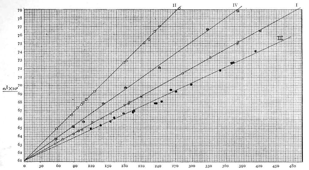
Fig 13

These results establish with absolute conclusiveness the correctness of the assertion that the apparent value of the electron is not in general a function of the gas in which the particle falls, of the materials used, or of the radius of the drop on which it is caught, even when that drop is of mercury, and even when it is as small as some of those with which Dr. Ehrenhaft obtained his erratic results. If it appears to be so with his drops, the cause cannot possibly be found in actual fluctuations in the charge of the electron without denying completely the validity of my results. But these results have now been checked, in their essential aspects, by scores of observers, including Dr. Ehrenhaft himself. Furthermore, it is not my results alone with which Dr. Ehrenhaft’s contention clashes. The latter is at variance also with all experiments like those of Rutherford and Geiger and Regener on the measurement of the charges carried by - and -particles, for these are infinitely smaller than any particles used by Dr. Ehrenhaft; and if, as he contends, the value of the unit out of which a charge is built up is smaller and smaller the smaller the capacity of the body on which it is found, then theseparticle charges ought to be extraordinarily minute in comparison with the charges on our oil drops. Instead of this, the charge on the