INVESTIGATION OF ATMOSPHERIC DOMAINS WITH THE AID OF MATHEMATICAL MODEL OF THE GLOBAL BIOGEOCHEMICAL CARBON CYCLE IN THE BIOSPHERE

INVESTIGATION OF ATMOSPHERIC DOMAINS WITH THE AID OF MATHEMATICAL MODEL OF THE GLOBAL BIOGEOCHEMICAL CARBON CYCLE IN THE BIOSPHERE

Tarko A.

Doctor of Physical and Mathematical Sciences, Professor of Mathematical Cybernetics Chief Researcher of the Dorodnicyn Computing Centre of the Federal Research Center «Computer Science and Control» of Russian Academy of Sciences

DOI: 10.24412/3453-9875-2021-70-1-10-22

Abstract

With the aid of mathematical model of global biogeochemical carbon cycle with a spatial structure and seasonal dynamics atmospheric C02 domains investigated. It is shown that domains which are the regions of low carbon dioxide concentration in the atmosphere arise as a result of the high photosynthetic activity of terrestrial vegetation in the interaction with the circulating atmosphere. Domains are gradually occupy a several spatial zones of low CO2 concentration from one edge of the Earth's map to the other.

Keywords: Modeling of the biosphere, biogeochemical cycles of carbon, net primary production, atmospheric transport, CO2 concentration, CO2 domains, tube of trajectories, contour lines.

Nowadays numerous measurements the biosphere parameters are being carried out in the world, as well as mathematical modeling of the global carbon cycle. However, much in understanding the properties biosphere remains unclear by this time and one of that is the integral functioning of the carbon cycle. The use of new measurements results and modeling of the carbon cycle allows us to obtain and test hypotheses about the functioning of the biosphere within a single spatial model and consider the biosphere as if it were the biosphere itself. This allows us to develop and test hypotheses about the dynamic properties of the biosphere, as well as to put forward new ones and immediately test them. Only on global models can we perform computational experiments with the biosphere that allow us to understand its holistic properties, provided that global experiments with the entire biosphere are impossible in reality.

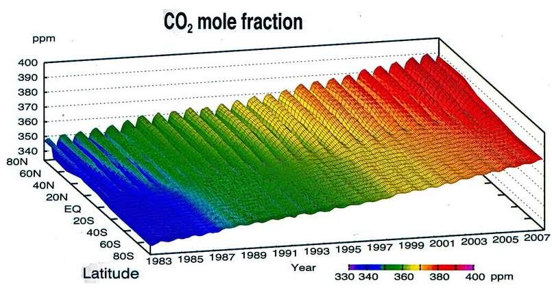
Usually, when analyzing the seasonal dynamics of the atmosphere, the dynamics of CO2 concentration is analyzed by latitude, and then the results are compared at different latitudes (Fig. 1). The subsequent work consists in determining the distribution of CO2 maxima and minima at each latitude and determining how far the CO2 minimum is far from the photosynthesis maximum at the same latitude. This approach does not provide a holistic understanding of the spatial dynamics of CO2 in the atmosphere.

Fig. 1. The 3D picture shows results of measurement of CO2 dynamics in the atmosphere. We can see seasonal fluctuations of CO2 every year and the change in the amplitude of fluctuations during the year at any latitude and also for several years (1983-2007) at each longitude.

In this article, with the help of mathematical modeling of the biosphere the author presents the results of a spatial study of the dynamics of CO2 in the entire atmosphere. The results obtained by such modeling on a global spatial biogeochemical model of carbon dioxide with seasonal dynamics. The author perhaps was the first to identify and study six regions of low carbon dioxide content in the atmosphere and called then domains. This study is devoted to the investigation of the formation and movement of CO2 domains in the atmosphere as part of the biosphere processes.

The research tool is a spatial mathematical model of the global biogeochemical carbon cycle developed jointly with V. V. Usatyuk [6, 7]. Biotic and physicochemical processes of carbon transport in terrestrial ecosystems, in the ocean and in the atmosphere are modeled. The model has a spatial resolution with a size of 4°x5° ongeographical grid, the time resolution is one day. Each land cell is considered to belong to one of the 30 types of ecosystems in accordance with the classification [1]. The General Circulation Model (GCM) in the atmosphere and ocean is used as a source of climate data [12].

This model is a variant of a more complicated biogeochemical model of the global CO2 cycle, which has also a more detailed resolution of 0.5°x0.5° and is used to study the stability of the biosphere and to analyze global warming processes [3, 4, 5].

The equations describing the dynamics of carbon in the vegetation cover take into account the following phase variables: the amount of carbon in the biomass of leaves, the biomass of trunks and the biomass of roots. The amount of carbon in the assimilates and the amount of water in the upper meter layer of the soil are also taken into account. The specific intensity of photosynthesis is calculated using the Gaastra equation. Respiration of plant organs and soil also is taken into account. Vegetation evapotranspiration is calculated using the Paynman-Monteith formula, which takes into account the energy balance of the moisture evaporation process.

In addition of GCM model special atmosphere block for calculating the transport of CO2 in the atmosphere has been developed. For this purpose, the convective-diffusion displacement of a small impurity of a passive gas in a given spherical velocity field was mathematically solved. The mathematical problem of convective-diffusion transfer of a small impurity of a passive gas in a given spherical velocity field is solved. Having its own transport unit allows the author to model the seasonal dynamics of CO2 concentration for each climate scenario, without performing a laborious calculation of all climatic parameters using a complete climate model.

The "atmosphere-ocean" block [2] is designed to calculate the parameters of the carbon cycle in the ocean, as well as to determine the carbon fluxes at the interface between the atmosphere and the ocean.

The model is validated using measurements of climatic and biotic parameters, data on the concentration of CO2 in the atmosphere at monitoring stations [1, 8, 11]. A check of the coincidence with the data of the spatial model was also carried out [5].

Computational experiments with satisfactory accuracy confirmed the course of the production process in land vegetation, in the decomposition of soil organic matter in most cells and allowed to obtain calculations of changes in the concentration and transport of CO2 during the year for all selected cells, as well as for latitudinal zones. Calculations have shown that the theoretical curves and measurement data are close both in amplitude and phase, i.e. this model satisfactorily reproduces the overall dynamics of CO2 in the atmosphere.

The computer simulation confirmed the hypothesis that the main causes of seasonal CO2 fluctuations are the photosynthetic activity of highly productive terrestrial vegetation, which releases a large amount of CO2 from the atmosphere, and also “pulls” CO2 from regions with lower photosynthesis values thousands of kilometers away.

In the model, the transfer of air masses along the latitude is much faster than in the meridional direction. Accordingly, the alignment of the CO2 concentration along the latitude also occurs much faster. For this reason, it is generally accepted in many studies that the composition of the atmosphere changes only in the meridional direction, but is the same throughout the latitude.

With the help of modeling, the author found stable structures in the atmosphere consisting of CO2 with a reduced CO2 content, which regularly occur in the atmosphere throughout the year. These structures are called domains. They occur in the atmosphere in different places at different times of the year, they contain local CO2 minima, and as they develop, they move and increase in size [6, 7]. 6 domains have been identified that occur in the following regions: 1) Europe and Siberia, 2) North America, 3) Amazonia, 4) Central Africa, 5) Indochina and 6) Australia and Indonesia (Fig. 2).

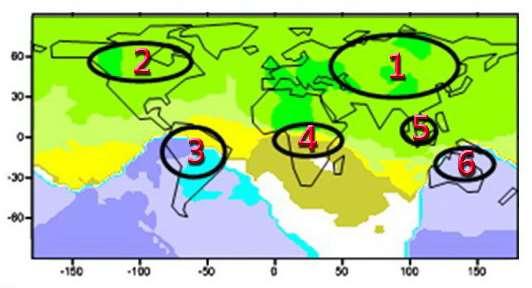
Fig. 2 Location of domains on a map of the Earth. 1 - Europe and Siberia, 2 - North America, 3 - Amazonia, 4- Central Africa, 5 - Indochina, 6 - Australia and Indonesia.

Domains appear as regions of an abnormal decrease of CO2 concentration against the background of its general dynamics, which have existed ordinary for a several months.

The phenomenon of domains was investigated using simulating experiments on the model which is described here. It was found that the main cause of the emergence of domains are production processes in highly productive ecosystems of terrestrial biota.

The atmospheric circulation has a significant effect on the characteristics of domains and their dynamics, due to which the domains are usually shifted towards the leeward border of the regions. Thus, they turn out to be “tied” to regions occupied by highly productive ecosystems, but do not occupy a strictly defined position above the surface of the Earth. Their position and shape is determined by the movement of air masses in the considered land region and depends on the intensity of carbon absorption by vegetation. Due to variations in climatic parameters, each year the vegetation season passes with different characteristics, therefore the shape of domains varies slightly in different years.

As already mentioned, usually when analyzing seasonal dynamics, the atmospheric CO2 concentration is averaged over latitude, and these curves are compared at different latitudes. In this paper, the author conducts a more complex analysis – there is a study the spatial movements of domains at the background of seasonal fluctuations in atmospheric CO2. One of the areas of research was the analysis of the spatial dynamics of processes in latitudes. To do this, there were constructed graphs representing the tubes of trajectories of atmospheric CO2 located at the same latitude during the year in each of 12 months for all longitudes (5 degrees of geographical coordinates). Thus, tubes of trajectories were constructed for latitudes N 60°, N 50°, N 30°, N 18°, S 10°, S 30° (Fig. 3).

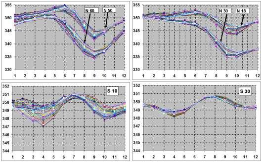
Fig. 3. Tubes of the trajectories of atmospheric CO2 concentration during the year at latitudes N 60°, N 50°, N 30°, N 18°, S 10°, S 30°. Each tube of the trajectories gives 72 curves of CO2 concentration of all longitudes (along 5 degrees) at given latitude. The vertical axis show atmospheric CO2 concentration in particles per million (ppm). The horizontal axis shows month numbers.

For all latitudes of the Northern Hemisphere from N 60° to S 10°, minimum of concentration are observed in September-October (for latitude S 10°, individual minima of the tube of trajectories reach November). Only at latitude S 30° do the values of the curves come in December-January to a state close to stationary.

The origin of these minima is explained by the fact that highly productive forest ecosystems of the Northern Hemisphere, located in the latitudinal range from N 40° to N 60°, absorb CO2 from the atmosphere in summer. The discrepancy between the time of the minimum of CO2 and the maximum of productivity by a month and a half is determined by the nature of the dynamic process in which the absorption of CO2 from the atmosphere has a maximum, but it shifts from the movement of air masses.

It should be noted that the far the south of the zones of the production process, the later the minimum is reached in the months indicated. The explanation of the results is that the zones of the active production process “attract” CO2 from neighboring atmospheric regions, and the effect of attraction extends to the north and south, spreading to the southern hemisphere.

It should be noted that ecosystems lying in the zone of boreal and subboreal forests of the Northern Hemisphere are of decisive importance for the occurrence of CO2 minimum. Ecosystems of the tropical zone, having higher productivity, exhibit weak seasonal variability, which does not allow influencing the formation of the time of onset of minima.

These highly productive zones are also present in the Southern Hemisphere, but they have much smaller sizes and power. The tubes of the trajectories S 10°, S 30° show unique complicated behavior At latitudes S 10° – 30° there is a double process. One process is the aforementioned “pulling” of CO2 by ecosystems of the Northern Hemisphere with a minimum of CO2 in September – October, and the other is the absorption of CO2 by “their” ecosystems with a minimum in March – April. This can be seen from the CO2 minimums on the tubes of trajectories S 10°, S 30°, reached in March – April, which also obviously lag is two months behind the maximum productivity in this hemisphere.

The reason for the large difference in the spread of CO2 values at the times of the minimum in the indicated months is unclear – at the latitude S 10° the “thickness” of the trajectory tube is much larger than at S 30° vary greatly at different longitudes. This case requires further, more careful research in modeling.

How are these results related to the previously identified six spatial domains? We can say that the domains are located inside the tubes of the trajectories of concentration of the course of atmospheric CO2 concentration during the year at latitudes. Indeed, each tube of trajectories means, as it were, an instant cut of 72 longitudes in each of the 12 months of the year. This procedure is not able to take into account domains that are spatial formations in the atmosphere. The consideration of the trajectories brings us closer to the assumption of instantaneous latitudinal mixing, accepted by the world when analyzing atmospheric CO2 monitoring data, but still does not reach this point.

Next, “surfaces” that form CO2 concentration values were examined. A series of computational experiments were performed with the condition that vegetation is occupying only one of several continents. For this purpose, the division of the land surface into four regions by geographical type is used: 1) Eurasia, 2) North America, 3) South America, 4) Africa. The outlines and boundaries of all areas are shown in Fig. 4. For each region the modeling was carried out until a periodic stationary regime was established, provided that the amount of carbon in all the system was constant. For each day, maps with isolines of atmospheric CO2 concentration and formed CO2 surfaces were constructed using the Surfer program.

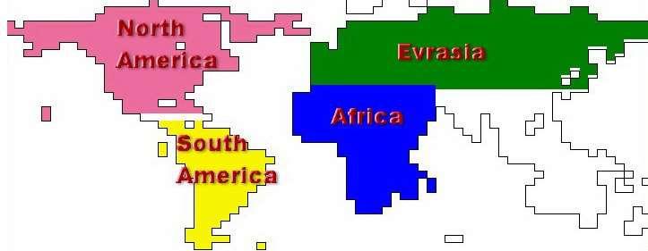
Fig. 4. Map of selected areas for partitioning the territory for modeling

We begin the study by analyzing processes in Eurasia. Vegetation season here begins in April – May. Usually, the first few days are accompanied by a uplift of CO2 into the atmosphere. This is due to the fact that the respiration of the soil, trunks and tree branches exceeds photosynthesis that occurs in the newly emerged leaves. Several days after and for the entire growing season, the CO2 uplift becomes directed from the atmosphere to the biota of the selected area. The following are maps with isolines and surface concentrations of atmospheric CO2 calculated using the model, calculated on the 180th, 200th and 260th days.

In fig. 5 (day 180), we see a noticeable decrease in CO2 lying in the range 0° – 180° E and a slight decrease in the northern part of the Western Hemisphere are also visible. This is due to the emergence of a domain (local minimum) upon absorption of CO2 by biota. The domain immediately begins to expand due to an increase in the intensity of the production process and turbulent diffusion of carbon dioxide in the atmosphere and is

carried away by the winds mainly to the east and partially to the south. With the development of the growing season, the domain continues to grow in size, while the resulting "funnel" from CO2 becomes deeper, its width increases in the latitudinal and longitude directions. The latitudinal direction is much larger, because the zone occupied by photosynthesis, increasing in all directions, especially grows towards the east. The main transfer of CO2 to the east comes from the fact that in the atmosphere due to the rotation of the Earth there is a shift of air masses to the east.

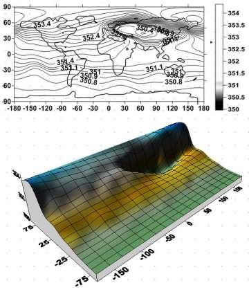
Fig. 5. Eurasia, day 180. Map and surface of CO2 concentration. A dip lying at 0-180° E and a slight decline in the northern part of the Western Hemisphere are visible. CO2 concentration decreases markedly from the North Pole to the South Pole.

The zone of lowered CO2 gradually reaches the Western Hemisphere, and on the map by the 200th day (fig. 6) a decrease in CO2 occurs in its left part. Two minimums are visually obtained – one reaches the border of the Eastern hemisphere (on the right of the map), the other moves from the left border of the Western hemisphere and goes to east (to the right). Then, as the size grows and shift eastward to 260 days, then two sections gradually merge into one wide zone (Fig. 7), reaching the North Pole in latitude to the north, and 2530° N in the south. Gradually, a large wide and deep band of reduced CO2 is obtained, while the decrease in the surface of CO2 reaches 25° S and there is also an increase in CO2 concentration in the circumpolar part of the Southern Hemisphere, due to the fact that the amount of CO2 in the simulated system does not change, and excess CO2 is transferred to the South.

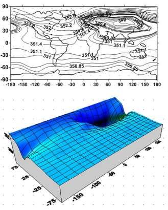
Fig. 6. Eurasia, day 200. Map and surface of CO2 concentration. A dip lying at 0° – 180° East. and a noticeable decrease in CO2 in the northern part of the Western Hemisphere are visible. CO2 concentrations in the northern and southern parts of the Earth are approximately equal.

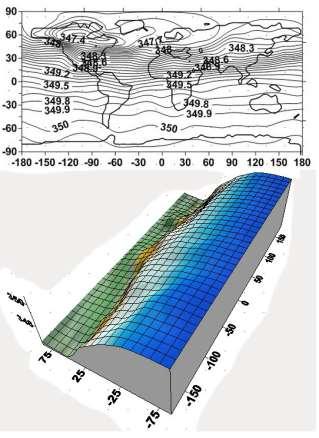
Fig. 7. Eurasia, day 260. Map and surface of CO2 concentration. Two CO2 minima are visible at the edges of the Eastern and Western hemispheres. Both minima are in a wide zone of low CO2 concentration formed by vegetation of biota. The CO2 concentration is rapidly growing from a wide zone of lower values at the North Pole to the South Pole.

The indicated circumstances are visible in fig. 8, which shows the difference in concentrations between 140 and 240 days of the year. On the map of contours and the surface of CO2 formed by the difference in CO2 concentrations, a minimum is seen that lies in the eastern part of the Northern Hemisphere, with a decrease in the CO2 difference of -10 ppm. In the western part of the map and the surface, a section of lowering CO2 is visible coming from the Eastern Hemisphere. The difference in CO2 concentrations from the northern part of the Earth increases markedly to the southern part. The zone of negative difference lies from the North Pole to 25° S. Note that in the system under study, the difference in CO2 concentrations does not reach negative values due to the fact that, as was mentioned, the amount of CO2 in the biosphere is constant and all variables cannot become negative.

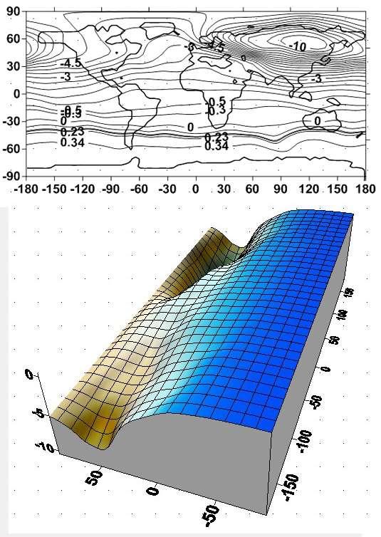
Fig. 8. Eurasia. Map and surface of CO2 concentration formed by the difference in CO2 concentrations in days 140 and 240 are presented. One can see a minimum of CO2 lying in the eastern part of the Northern Hemisphere, with a (-10) ppm of CO2 concentration. In the western part of the map and the surface, a section lowering of CO2 is visible coming from the Eastern Hemisphere. The difference in CO2 concentrations from the northern part of the Earth increases noticeably to the southern part. The zone of negative difference occupies the space from the North Pole to 25°S

Fig. 9-10 shows maps of the "North America" scenario with isolines and surface of atmospheric CO2 concentrations on the 200th, 240th, and 260th days. In general, we obtained qualitatively similar results with the "Eurasia" scenario. The difference is that the source of the production process is located to the west, while the territories occupied by vegetation is less space in longitude, and in latitude is closer to the south. Fig. 9 shows a similar to fig. 5 noticeable decrease in the concentration of CO2 in the area by the 200th day of the year. Then, over time, the zone of reduced CO2 gradually reaches the edge of the Eastern Hemisphere and the border of the Western hemisphere. At the same time, two minima do not appear on the map, there is no place for this on the territory of America.

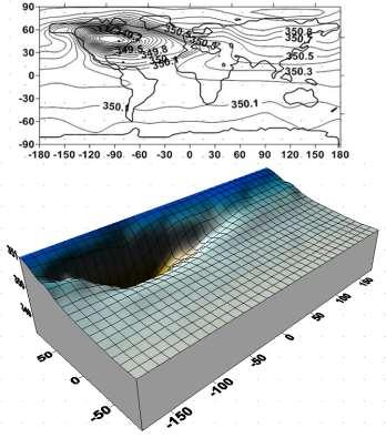
Fig. 9. The scenario “North America” Day 200. Map and surface of CO2

The influence of the domain is such that the concentration of CO2 is reduced towards the North Pole. The area with a minimum of CO2 gradually turns into one wide zone (Fig. 10-11), reaching the latitude to the north – the North Pole. Gradually, a large wide and deep band of reduced CO2 is obtained. In this case, just as in "Eurasia", the absorption of CO2 in the domain leads to the fact that the direction of the north – south shift of the CO2 concentration significantly decreases towards the North Pole.

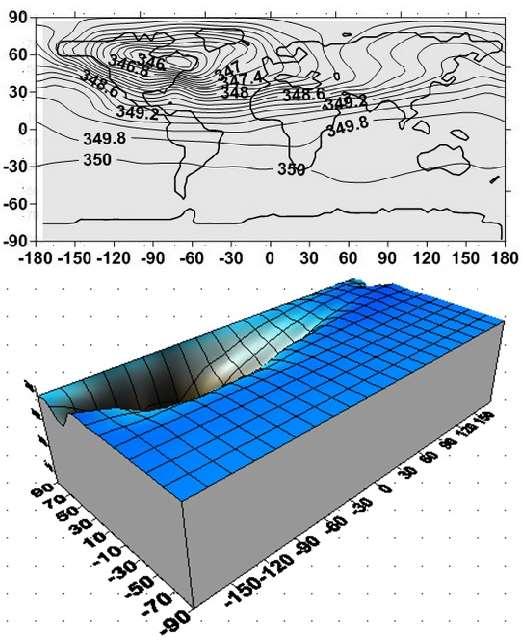
Fig. 10. The scenario "North America" Day 240. Map and surface of CO2

Fig. 11. Scenario "North America" Day 260. Map and surface of CO2

In Fig. 12-13, the results of the “South America” scenario calculations with contours and surface of atmospheric CO2 concentration on the 160th and 50th days are given. Fig. 12 shows noticeable decrease in CO2 concentration in the zone of equatorial tropical forests, from which territories of low CO2 concentration go west and east to borders of the map. Another case is shown in Fig.13: the zone of reduced CO2, still occupying tropical forests, gradually decreases towards the producing vegetation of the Southern Hemisphere, while there is also a sharp decline of CO2 in zone W 50° longitude to the South Pole.

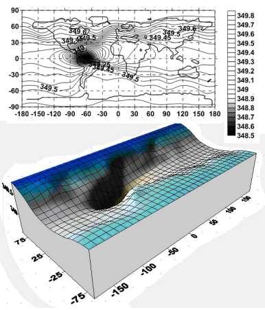
Fig.12. Scenario "South America". Day 160. Map and surface of CO2

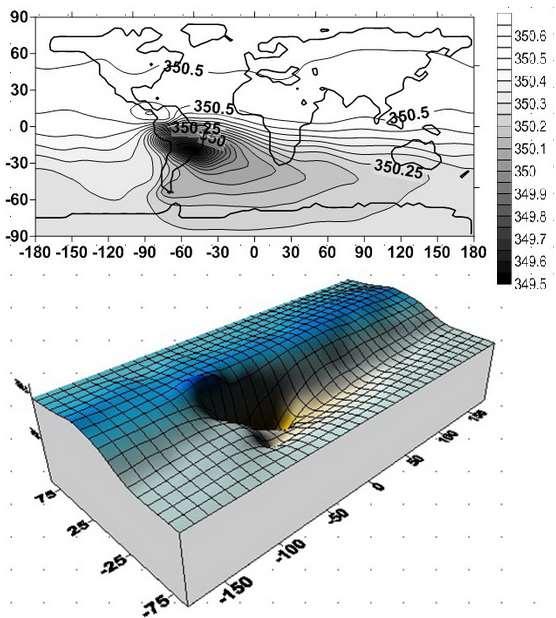
Fig.13. Scenario "South America". Day 50. Map and surface of CO2

Fig. 14 shows the calculation map of the "Africa" scenario with isolines and surface of atmospheric CO2 concentration on day 320. Fig. 14 shows the influence of the equatorial tropical vegetation of Africa. A strong decrease in the CO2 concentration in the tropical vegetation zone is visible, and a wide band of reduced CO2 concentration is visible, extending to the North Pole and reaching the eastern and western borders of the map. In this scenario, the same effects that have already been played are reproduced. The vegetation south of the tropical zone is particularly affected. At the same time, the minimum of CO2 in the Northern part of Africa is accompanied by a gradually decreasing concentration of CO2 in the Southern Hemisphere. There is a stronger change in the direction of the CO2 concentration of vector "Northern – Southern" hemisphere.

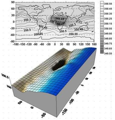
Fig.15. Scenario "Africa". Day 50. Map and surface of CO2

Fig. 16 shows isolines of the CO2 of the "Africa" scenario at map of difference between 320 and 140 days. It can be seen that almost the entire land area between the poles has a reduced concentration. An exception is an uneven strip with a protrusion near the equator and a small area at the South Pole. Note that this figure demonstrates not only a change in the direction of the vector of the shift of the CO2 concentration "north – south", but manifests moments when its direction goes from the equatorial part to both poles of the planet.

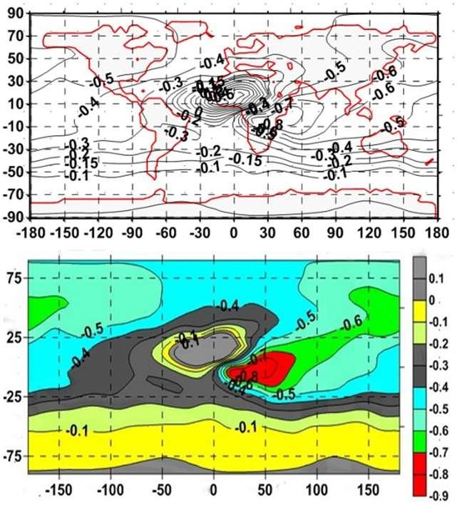
Fig. 16. The scenario "Africa". Isolines of the difference of the CO2 concentrations between 320 and 140 days

Thus, for the first time it was shown that each of the considered continents leads to the formation of significant territories involved in the process of CO2 transport in the atmosphere, exceeding half the planet’s surface. Domains formed over the continents gradually occupy a wide latitudinal band of low CO2 concentration from one edge of the Earth's map to the other. This strip can occupy almost the entire hemisphere from one continent and enter to another. At this case, during the year, the direction of CO2 reduction can be changed - it can be mainly directed to the Northern Hemisphere from the Southern Hemisphere, and visa versa. It is also possible that the decrease in concentration occurs from the equatorial region with a simultaneous decrease to the North Pole and to the South Pole.

From the simulation experiments, it became clear that the power of the processes of air mass movement associated with the photosynthetic activity of terrestrial vegetation is higher than when forming the interaction of two neighboring continents, based on the values recorded at monitoring stations. The curves of the dynamics of CO2 in the atmosphere are formed not only by two neighboring continents, but by almost all the continents of the Earth. The results of the calculations showed that the formation of the values of the CO2 minima strongly depends not only on the vegetation of the nearest continents, but on several at once.

The usual practice, when firstly the climate and the distribution of CO2 in the atmosphere are calculated, and then the calculations of the vegetation production process are performing with a constant or slightly changing atmospheric CO2 concentration, may be insufficient in some real situations. In particular, with severe violations of the production process in local or large regions on the land are. Examples can be cases of strong warming of the atmosphere during global warming or calculations of the consequences under some scenarios of a limited Nuclear Winter.

It is known that during the vegetation process, air masses bypass the Earth several times along the latitude. This means that the simulated CO2 flow curves are the result of a complex geophysical process of CO2 dynamics in atmosphere. However, what is the relationship between the properties of the domain dynamics identified here and the fact of multiple "round-theworld travel" of air masses during the year remains to be determined.

The author has a pleasure to expresses gratitude to Vladimir Usatyuk who helped author to carrying out computer calculations for this article.

REFERENCES:

1.Bazilevich N.I., Rodin L.E. Maps of productivity of the biological cycle of the main types of land vegetation // Proceedings of the All-Union Geographical Society.- 1967.- T. 99.- N 3.- p. 190-194. (In Russian). 2.Pervanyuk V.S. Tarko A.M. Modeling the Global Carbon Cycle in an Atmosphere-Ocean System. // Mathematical Modeling, 2001, v. 13, No. 11, p. 1322. (In Russian). 3.Tarko A.M. The global role of the atmosphereplants-soil system in compensating for impacts on the