Quantified Parameters

Global biodiversity scenarios: what do they tell us for biodiversity-related socio-economic impacts?

4. Key Assumptions and Quantified Parameters

Once a scenario narrative is complete, it can be transformed into a quantitative trajectory using models. Indeed, the storyline must be translated into a quantitative scenario, specifying values (constant or varying) for several model parameters. The model will also need other quantitative hypotheses to fix values of the parameters that do not belong to the specified scenario (this is also known as calibrating or estimating the model). However, moving from qualitative to quantitative scenarios often means that some dynamics are not measurable or not easily accounted for.

Almost all studies quantified Gross Domestic Product (GDP) and population trajectories (at least) from SSPs. Many of them also coupled the SSP assumptions with one or more Representative Concentration Pathways (RCPs) that describe future greenhouse gas (GHG) concentration for different climate scenarios until 2300 (van Vuuren et al., 2011).

A – The Gross Domestic Product (GDP) Quantification

The Organisation for Economic Co-operation and Development (OECD) approach for measuring GDP trends in the SSP trajectories is dominant. They opted for an augmented version of the Solow growth model, which does not include natural resources and land-use other than crude oil and natural gas as growth factors. Namely, if no land is available to expand agriculture and the land currently being farmed is too degraded, the country’s long-run production and/or value-added will not be affected.

Moreover, their model assumes conditional convergence. It means that, from the first year of the projection, the GDP of least developed countries will increase more rapidly than those of developed countries, leading to convergence (catchup effect). As a result, GDP growth trajectories are positive for every country at least until 2100 (both in total and per capita term) even though the scenario envisaged proposes a significant structural change (either an ecological transition or collapse of biodiversity) which should precisely affect long-term growth. It is however likely that the dramatic changes in direct and indirect drivers of biodiversity loss and mitigation policies implied by the scenarios will result in a decrease in global GDP, or at least for some countries that fail to adapt to an ecological transition or experience an ecosystem collapse. The only attempt to recast SSPs for exploring low, zero, and negative GDP growth by coupling biodiversity loss to economic growth, i.e., by incorporating the possibility of limited growth due to natural resource degradation, is that of Otero et al. (2020). However, these storylines have never been quantified.

B – An Overview of Possible Quantitative Policies and Trajectories per “Sectors”

On top of SSP trajectories, most authors added various pathways, political/behavior shifts, or collapse assumptions; they incorporated strategies for biodiversity conservation, ecosystem restoration, food security, or global warming mitigation. However, some authors did not necessarily couple SSP with biodiversity conservation policies and only looked at the impact of SSP on biodiversity (Schipper et al., 2020; Pereira et al., 2020). All these assumptions and quantified parameters are mostly embedded in the following sectors or areas of focus.

The agricultural sector

The agricultural sector is crucial in biodiversity scenario development because it affects biodiversity the most, notably by converting natural habitats to intensely managed systems and releasing pollutants: crops and livestock production occupy 50% of the global habitable land surface (excluding ice-covered land).

The trajectories attributed to this sector are mainly supply-side, and trajectories related to the agricultural sector productivity (e.g., crop yield, irrigation, and fertilizer efficiency) are the most widely modeled. Usually, crop productivity without additional inputs (i.e., fertilizer and waste) in developing countries is projected to converge to the level of developed countries, even if it will require a lot of investment and innovation. Crop productivity may also be constrained by climate change impact on soils (Rosenzweig et al., 2014), which is often not accounted for in the scenarios.

Global biodiversity scenarios: what do they tell us for biodiversity-related socio-economic impacts?

The authors also added policies to limit harmful subsidies or increase taxes on the agricultural sector. For example, Johnson et al. (2021) quantified the removal of all subsidies from the agricultural sector in favor of a system of lump-sum transfers to farmers, and Kok et al. (2020) quantified the introduction of a 10% import tax on all agricultural products by 2050. However, as agricultural products are internationally traded, those interventions necessitate a global implementation and, therefore, total cooperation between countries. However, SSP narratives do not propose the same degree of collaboration between countries.

Some demand-side policies are nevertheless modeled; they are primarily related to changes in food production, such as reducing food losses (from harvesting, processing, distribution, and final household consumption) and changes in the consumption of animal products. For example, Kok et al. (2020) and Leclère et al. (2020) simulated a 50% reduction in food loss and animal calorie consumption by 2050 based on current country trends.

Policies that target the agricultural sector are very broad and do not differentiate between the different agricultural practices that exist. We will see later that the concern is with models of direct and indirect drivers of change that are unable to provide accurate information on sectors and sub-sectors. Land-use trajectories

A flagship measure of the CBD in the “Post-2020 Biodiversity Framework” is the protection and conservation of species habitats through the expansion of PAs and Other Effective area-based Conservation Measures (OECMs)6 to protect at least 30% of the terrestrial surface by 2030. Currently, PAs and OECMs cover only 17% of the world’s land and inland water surface but depending on the country, the proportion can vary from 1% to 50%7 .

Therefore, expanding PAs and OECMs is the most widely modeled biodiversity conservation policy. However, because no consensus exists globally on what percentage of land should be regulated and where, researchers make their own decision, guided by existing literature and desired outcomes.

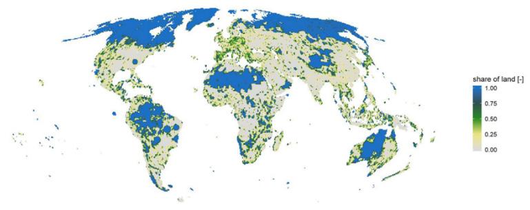
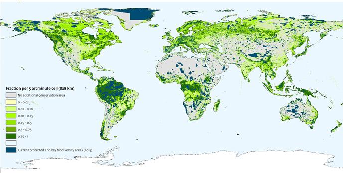
Depending on the scenario, the assumptions range from 30% to 50% of terrestrial PA expansion, but their distribution differs widely. For example, we compare the 30% PA expansion policy of Kok et al. (2020) with the 40% expansion policy designed by Leclère et al. (2020), see Figure 2. We can see that the latter is “politically” easier to implement but not at all convincing from an ecological point of view. Indeed, the conservation effort shifted to the northern boreal zones and the desert zones of Australia and the Sahara in Africa, sparing, for example, the tropical forests of the Congo Basin, which represents a key zone in terms of biodiversity. Yet the CBD emphasizes the need to select PAs based on their importance for biodiversity and their contribution to people for conservation to be effective and equitable.

6 An Other Effective area-based Conservation Measure (OECM) represents a geographically defined area other than a PA, which is governed and managed in ways that achieve positive and sustained long-term outcomes for the in-situ conservation of biodiversity, with associated ecosystem functions and services and where applicable, cultural, spiritual, socio–economic, and other locally relevant values.» (Definition agreed at the 14th Conference of Parties of the CBD in 2018). 7 Protected Planet. https://www.protectedplanet.net/en.

Figure 2 - (A) Conservation areas for the Sharing the Planet scenario with the ambition to conserve 30% of the global land and freshwater area by 2050 (Kok et al., 2020); (B) Conservation zones for PA expansion policy with the ambition of conserving 40% of the land area by 2020 (Leclère et al., 2020).

In addition, establishing an effective PA network is costly. It can include monitoring habitat health, enforcing regulations, and investing in research fees to prevent illegal activities in PAs, such as logging, poaching of protected animals, mining, and encroachment by human settlements and agriculture. Nevertheless, they offer economical and social benefits and mitigate the economic risks of climate change even if not all countries will have the capacity to capture them, particularly in terms of tourism development (Waldron et al., 2020). Overall, Johnson et al. (2021) estimated that achieving the protection of 30% of the world’s lands would require an average annual investment of about $115 billion until 2030. Still, if the benefit of avoided carbon emissions is included, it is reduced to $13 billion. The cost and benefits associated with the expansion of PAs are however rarely considered in the scenarios.

A

B

Global biodiversity scenarios: what do they tell us for biodiversity-related socio-economic impacts?

The type of protection envisaged in the PAs, such as whether or not human activities can be developed within them or what kind of activity is allowed (e.g., recreational and forestry), is not always clearly defined in the scenarios. However, these factors will potentially significantly impact the speed and magnitude of biodiversity degradation and economic outcomes.

The high-sea fishing sector and sea-use trajectories

The policies and trajectories implemented to improve marine biodiversity are diverse and creative. They focus, for example, on subsidies, ex-vessel fees, Marine PAs (MPAs), or fisheries management techniques shifts.

For example, Cheung et al. (2019) quantified and adjusted three SSP narratives notably by adapting trajectories on ex-vessel prices of marine species, subsidy changes, fishery operating and investment costs, and catchability rates. For all these scenarios, MPA expansion constraints of 0-50% are simulated by 2050, with a median target of 30% of the total high-seas area, and radiative forcing trajectories are defined (i.e., RCP 2.6 and RCP 8.5). However, current MPAs only cover about 8.15%8 of the oceans, so establishing 50% MPAs by 2050 will be challenging and will require a lot of monitoring and investment that is not accounted for in the scenarios. Moreover, as with terrestrial PAs, MPAs are likely to be costly and generate co-benefits (e.g., tourism and coastal protection) that are not accounted for in the scenarios.

Globally, no article distinguishes between different fishing sectors (i.e., recreational, subsistence, and commercial) and types of commercial fishing methods: whether an industry is fishing with nets (e.g., purse seine, trawling, and bottom trawl) or with line (e.g., longlines, pole, and line) or harvesting shellfish. Nevertheless, all these parameters will have different consequences in terms of biodiversity erosion and capacity to satisfy the growing seafood demand. Additionally, it does not allow for the differentiation of fishing activities and, therefore, the identification and valorization of techniques that are less destructive of marine ecosystems (i.e. identification of transition opportunities). The forestry sector

Researchers explored measures to mitigate global warming by maintaining carbon storage through avoiding deforestation in the scenarios. These policies always assume full cooperation and coordination between countries. For instance, Johnson et al. (2021) identified two different trajectories depending on the scenario. In the former case, payment for forest carbon is made within each country by limiting the supply of land and compensating forest owners through increased land subsidies. In the second case, payment for forest carbon is realized by rich countries based on their historical GHG emissions, and payment is received by poorer countries based on avoided deforestation.

The energy sector

Only a few studies have set up trajectories targeting the energy sector. For instance, Obersteiner et al. (2016) simulated two different policies to achieve the 2°C global warming target by imposing either a moderate share of bioenergy and nuclear power or a high percentage of bioenergy and no nuclear power by 2030.

Contrary to the climate scenarios for which this sector is crucial, biodiversity is less impacted by a single industry. As a result, the studies integrate a few climate change mitigation and adaptation policies (e.g., through the forestry or the energy sector). We, therefore, recommend building a bridge between climate and biodiversity scenarios, especially to identify the potential for compounding and cascading impacts on the economy.

Nevertheless, scenarios focusing on biodiversity change allow us to understand which policy intervention will be the most effective in conserving biodiversity. Indeed, some measures to mitigate global warming do not produce “co-benefits” for biodiversity or even degrade it further and vice versa. For example, the expansion of hydropower plants, intensely simulated in climate scenarios, provides clean electricity with low GHG emissions, but at the same time, it degrades biodiversity (e.g., by fragmenting watercourses and disrupting certain biological cycles).

8 Protected Planet. https://www.protectedplanet.net/en.

C – Collapse Assumptions

Johnson et al. (2021) designed the only exploratory physical scenario in the literature review. They designed a collapse of multiple ESs due to extreme environmental shocks. They simulated the effect of a 90% reduction in wild pollination on agricultural yields (i.e., the collapse of pollinator ESs) only for crops dependent on wild pollination.

Moreover, they designed a collapse of marine fisheries. As a result, they implemented a severe climate change scenario (RCP 8.5) to simulate drastic disruptions in fish migration that would result in a reduced total catch in terms of biomass, which registers as a technology-neutral productivity change in the fishing sector.

In addition, Johnson et al. (2021) modeled a sudden collapse in timber production. They assumed an 88% decrease in forest cover for all tropical regions and suggested a decline in the ability to expand forestry in humid tropical areas with a longer growth period.