1. An Environmental Lewis-Prebisch-Thirlwall model

The last years have seen important developments in ecological macroeconomics and, more specifically, in the development of models consistently integrating economy-environment linkages. Most of these attempts describe the world economy 2, thereby leaving aside the specificities that small open economies face in the context of the green transition. However, there have also been attempts to incorporate ecological considerations into models describing the perspective of a peripheral economy (Dunz and Naqvi, 2016; Guarini and Porcile, 2016; Althouse et al., 2020; Gramkow and Porcile, 2022). The model presented in this section is closely related to the latter strand of the literature.

The model builds on Porcile and Spinola (2018), who in turn draw on the framework developed by Setterfield (2011). Being a long-run framework, the goal is to explore the properties of the position where the economy would tend to be when the short-run-related noise is absent. Thus, the equilibrium rates derived from the model can be interpreted as those attainable in a sustainable way, i.e., in a situation where all the constraints embedded in the model are being fulfilled. In particular, the aim of Porcile and Spinola (2018) is to explore the alternative closures that ensure that long-run demand-driven growth is consistent with the balance of payments constraint and with supply-side conditions (in other words, they define different adjustment mechanisms through which the natural, the effective and the balance of payments equilibrium growth rates are equalized in the long-run).

In this paper, we take the Lewis-Prebisch-Thirlwall closure proposed by Porcile and Spinola (ibid), implying that long-run economic growth is determined by the balance of payments equilibrium as suggested by Thirlwall (1979) for the reasons originally laid down by Prebisch (1950). Thus, the long-run aggregate demand growth will find an upper limit in the balance of payment equilibrium. Following Lewis’ (1954) contributions, a two-sector economy is assumed: a modern sector with high wages and a traditional and predominantly informal with a large “reserve army” and, hence, with low wages. The Lewisian element of the model is given by the way the supply side adjusts to demand. It is assumed an infinite elasticity of labour supply to the relative wage between sectors, implying that the labour supply (and hence the natural rate of growth) is endogenous such that long-run equilibrium between supply and demand is ensured. Porcile and Spinola propose other interesting closures where, for instance, productivity is endogenized so that the supply-side adjustment to demand can be made through a process of structural change. However, given the motivation of this paper it seems more reasonable to assume a static productive structure such that the starting point of South American economies' green transition, as well as the trajectory that brought them to it, is best represented

2 For instance, Taylor et al. (2016) build a demanddriven growth model involving capital accumulation and the dynamics of greenhouse gas concentration to examine the macroeconomic issues raised by global warming, while

Dafermos et al. (2018) build a fully-fledged stockflow consistent model with a coherent integration of economic and environmental processes to analyze the effects of climate change on financial stability.

The short-run growth rate is demand determined and given by the growth rates of exports ����, and the growth rate of domestic demand ���� , each weighted by the parameters ���� and ���� , which are a function of their share of aggregate demand, as proposed by Setterfield and Cornwall (2002). The derivation of this equation can be found in the appendix.

���� ���� = �������� + �������� (1)

The growth rate of exports normally depends on the growth rate of the rest of the world ���� ���� multiplied by the income elasticity ���� , the rate of depreciation of the real exchange rate ���� and the price elasticity of exports �������� . In the long run the real exchange rate is in equilibrium, implying that ���� = 0 and that the exports equation can be simplified to ���� = ���� ���� ���� Since the growth rate of the rest of the world is exogenous and assuming a static productive structure (���� constant), the growth rate of exports can be assumed to be exogenous in the long run.

Balance of payments constrained growth implies, as defined in Thirlwall (1979), that the long-run growth rate of GDP is given by the growth rate of the rest of the world multiplied by the ratio of exports and imports income elasticities (���� and ����, respectively). As many authors of the Neo-structuralist school have claimed, the ratio ���� ���� is a function of the technological capabilities of the economy or, in other words, the complexity of its productive structure. The higher the technological capabilities, the more effectively the economy will respond to the rest of the world´s demand (Araujo and Lima, 2007; Cimoli and Porcile, 2014).

Being ���� �������� , as suggested by Blecker (2013), the long-run “attractor” of the growth rate of GDP, it is necessary to define how aggregate demand converges to it. Porcile and Spinola (2018) assume that the growth rate of domestic demand converges to the balance of payments equilibrium growth rate at a speed ����, as shown in equation (3). ����

Assuming a production function comprising labour and technology and an unlimited stock of natural resources 3, the natural growth rate ���� ���� can be defined as the sum of the growth rate of labour supply ���� and the growth rate of technology ���� The Lewisian closure implies that labour supply is infinitely elastic, thereby closing any gap between production (in turn given by aggregate demand as shown in equation 1 with the binding balance of payments constraint (2)) and productivity growth. A more detailed description of the endogenous adjustment of the supply side, including the determinants of technology growth, can be found in the appendix.

3 The assumption of limitless natural resources is not realistic. However, it is kept to simply the analysis because, for the period for which the green transition is being debated (need to achieve carbon neutrality by 2050), Latin American countries are not expected to be subject to natural resource depletion. The impact of relaxing this assumption is left for future research.

Net greenhouse gas emissions growth ���� is given by the growth rate of aggregate demand components (���� and ���� ) and their carbon intensity (�������� for exports and �������� for autonomous demand) relative to the average carbon intensity of the economy (����), weighted by their share in output (����1 and ���� � , respectively). The change in greenhouse gas absorptions made by the country’s carbon sinks, ����, is also considered in the growth of net greenhouse gas emissions If the country’s carbon sinks absorption capacity is constant, then ���� = 0. If the absorption capacity is declining (for instance, due to deforestation), then ���� < 0. On the other hand, if the absorption capacity is increasing (for instance, as a result of reforestation or, in the future, geoengineering techniques), then ���� > 0 The complete derivation of equation (10) can be found in the appendix.

Inspired by Jackson and Victor (2020), who claim that a broader measure of wellbeing should be considered instead of per capita GDP, we define a simplified measure of prosperity function of income per capita ���� ���� /���� and pollution, which we proxy by per capita greenhouse gases emitted by the country, ���� /���� 4. The parameter 0 < ���� < 1 represents the country’s weight of the material and environmental dimensions of prosperity in determining total prosperity. If ���� = 0 5 both dimensions are given the same importance. Equation 6 presents the growth rate of prosperity, ����, as an increasing function of the growth rate of demand, and decreasing in the growth rate of population and pollution. Considering equations 1 and 5, the growth rate of prosperity ultimately depends on the growth rates of the components of aggregate demand, their share in it, and their greenhouse gas intensity. As long as the economy has not reached carbon neutrality (�������� = �������� = 0, implying that ���� = 0) there will be a trade-off between growth and environmental sustainability – the higher the growth rate of aggregate demand, the higher the resulting pollution levels. The derivation of equation 6 can be found in the appendix.

Given the structure of the model the green transition dilemma that South American countries face is already visible. To converge to higher levels of prosperity in the long run a higher growth rate of prosperity is needed in the medium run. Given the population growth rate, this requires that income levels grow at a high rate ( ↑ ���� ���� ) which, according to Thirlwall’s law, would need an increase in the growth rate of exports ( ↑ ����). Since the carbon intensity of exports of Latin American countries is higher than the one of domestic demand (�������� > �������� ), the increase in the growth rate of exports would lead to an increase in the rate of growth of greenhouse gas emissions ( ↑ ����), ultimately undermining the growth rate of prosperity (or eventually reducing it) and backfiring on the whole development strategy.

4 The sustainable prosperity index constructed by Jackson and Victor (2020) includes GDP per capita, the Gini index, hours worked, households’ loan-to-value ratio, the government debt-to-GDP ratio, and the unemployment rate. To make the model as simple as possible the proposed prosperity index is limited to income per capita and domestic greenhouse gas emissions. The reason why only domestic emissions (instead of global) are considered is that to focus on the development policy trade-offs and dilemmas we focus on the variables that the country can directly or indirectly affect.

On the other hand, the goal of attaining carbon neutrality (���� = ���� = 0) would imply, under the current productive structure (given by ����, ���� , ���� and ����), its carbon intensity (given by �������� and �������� ) and the absorption capacity (Θ), the need to reduce the growth rate of exports, thereby putting a low upper limit on ���� �������� and, therefore, on ���� ���� and ���� Thus, given their productive structure it seems that South American economies cannot simultaneously achieve both higher levels of prosperity and carbon neutrality. At the core of ”Gordian knot” is the balance of payments constraint.

3. Closure 1: Exogenously determined Exports

The traditional way South American countries took to obtain the resources they need to finance domestic consumption and, eventually, the investment required to pursue a process of structural change has been the exports of commodities 5. As mentioned before, it is a feature of natural resources-based activities, especially extractive ones, to have an above-average carbon intensity. Hence, a development strategy based on commodities exports, such that the country can increase its prosperity without hitting the balance of payments constraint, seems to be at odds with the transition toward a zero-carbon economy.

Assuming that the country’s exports are exogenously determined by the rest of the world’s growth rate times the income elasticity of exports, ���� = ���� ���� ���� , as specified in the previous section. In this case, given the parameters ���� and �������� there is no mechanism taking the economy to carbon neutrality in the long run. The convergence of the demand-driven output growth to the balance-of-payments equilibrium growth rate is given by equation (3). Still, nothing in this closure caps emissions (like, for instance, NDCs) and, therefore, the growth rate of exports. Note, however, that if the rest of the world embarks in a green transition (either through a de-growth process, represented by a fall in ���� ���� , or by a change in production and consumption patterns, which impacts on the country’s exports would be seen through a fall in ���� ) the country’s exports growth could also be negatively affected, thereby making the external constraint more binding and limiting the space to increase prosperity.

In such a situation, where exports grow at an exogenous rate, the country’s greenhouse gas emissions growth rate is endogenous, as defined in equation (5). This situation is, as a matter of fact, a description of how the joint evolution of the dynamics of exports and greenhouse gas emissions have been until now. Therefore, the dynamic system consists only of one equation (equation 3) Given that both ����, ���� > 0, stability will always be attained.

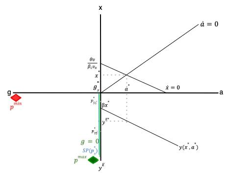
Figure 1 shows the main elements needed to analyze the implications of the export-led prosperity closure. We first use the figure in the left panel and leave the one in the right for later when changes in the societal preferences regarding environmental issues are explored. In the upper quadrant we plot the growth rates of exports, ����, and the rest of the elements of aggregate demand, ���� . The growth rate of exports is exogenously given by ���� and ���� ���� Together with the income elasticity of imports, ���� , these two parameters determine the balance of payments equilibrium growth rate which, in turn, defines the long-run equilibrium growth rate of the rest of the components of aggregate demand, ���� ∗ =

���� . The ���� = 0 locus shows the range of possible long-run equilibria. As the expression of ����∗ shows, the higher the growth rate of exports, the higher the possible growth rates of the rest of the components of aggregate demand, thereby leading to a higher level of total aggregate demand ���� ���� The slope of the ���� = 0 locus is given by the composition of aggregate demand (parameters ���� and ���� ) and the income elasticity of imports, ����. For instance, an economy where exports are not only crucial for growth as a source of foreign exchange but also as a direct source of demand (a high ���� ) would exhibit an ���� = 0 locus with a smaller slope, i.e., rotated clockwise compared to the one plotted in Figure 1, and implying a higher possible long-run growth rate of aggregate demand.

5 In the last decades capital inflows have become an increasingly important source of financing current account deficits, but as some authors have shown these inflows were to a large extent related directly or indirectly to the country’s status of commodity exporters.

Based on the equilibrium growth rates of exports and the domestic demand, the long-run equilibrium growth rate of income is obtained, ���� ���� ∗ . The bottom-right quadrant plots the income growth function as defined in equation 1. The intercept of the function is given by the equilibrium growth rate of exports weighted by ���� , which is a function of their share on aggregate demand. The higher the growth rate of exports, the higher the possible attainable growth rate of income, as the balance of payments constraint becomes less binding. The slope of the function is positive and given by ���� , showing that for a given equilibrium growth rate of domestic demand, the overall growth rate of income will tend to be higher the larger the share of domestic demand on aggregate demand

Based on the long-run equilibrium growth rate of demand obtained in the bottom-right quadrant it is possible to derive the associated growth rate of pollution (emissions) using equation 5 This is represented in the bottom-left quadrant, where the two varying arguments of the prosperity growth function, ���� ���� and ���� (we will let ���� be constant all over the subsequent experiments), are defined in the axes. For illustrative purposes two alternatives are shown. The first one is the more environmentfriendly or sustainable, which we call ���� ���� , is given by either low levels of the carbon intensity of exports, �������� , or of the domestic demand, �������� , by a high absorption capacity of the country’s carbon sinks, Θ, by a high weight on aggregate demand of carbon-intensive activities, or by a combination of all these elements. The second pollution function, which we call �������� , has the opposite features, thereby representing an environmentally unfriendly or unsustainable structure. The intercept of these two functions is negative (the exact value given by ����) because if output growth were zero, emissions growth would be negative (if Θ > 0). Projecting the long-run equilibrium growth rate of aggregate demand ���� ���� into the bottom-left quadrant we find the long-run growth rate of pollution, which is �������� ∗ for the sustainable case and �������� ∗ for the unsustainable one. As it can easily be observed, �������� ∗ < �������� ∗ , implying that for the same long-run growth rate of aggregate demand, prosperity growth will be higher in the (���� ���� ∗ , �������� ∗ ) equilibrium, as higher greenhouse gas emissions are negatively related to prosperity.

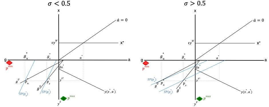
Recalling that prosperity growth was defined as dependent on income and pollution growth rates (equation 6), the level curves of the prosperity growth function can also be drawn in the bottom-left quadrant. Following Jackson and Victor (2020) we call these curves SP, standing for sustainable prosperity. From equation (6) it is derived that these level curves are linear, as illustrated in the blue lines. Their intercept depends on the growth rate of prosperity and the societal preferences regarding the weight of the material and environmental dimensions of prosperity. Higher (desired) prosperity growth rates (like, for instance, ��������∗ ) would be located in more rightward curves (like ��������(��������∗ )), showing that for a given growth rate of income (���� ���� ∗ ) lower (even negative) growth rates of greenhouse gas emissions would be required. On the contrary, a low growth rate of prosperity (like �������� ∗ ) would mean that the same growth rate of income could coexist with higher growth rates of greenhouse gas emissions. In a similar vein, if society prioritizes income growth over pollution reduction (���� > 0 5), the growth rate of income per capita ���� ���� ∗ can be attained tolerating higher growth rates of emissions, as the steeper level curves in the right panel show. Conversely, when society weighs more on environmental sustainability (���� < 0 5) the income growth rate ���� ���� ∗ needs to be attained with lower pollution growth, as the flatter curves in the left panel show The sustainable prosperity curves are drawn for both equilibrium levels of prosperity, �������� ∗ and �������� ∗ , which correspond to two different economic structures. As mentioned before, �������� ∗ > �������� ∗ , implying that the combinations of income and pollution growth comprised in the ��������(��������∗ ) curve are higher than the ones contained in the ��������(�������� ∗ ) curve.

Maximum prosperity growth is achieved when long-run income growth is high (implying that the country has enough room to catch up with developed countries) and greenhouse gas emissions growth is zero. In a growing economy this would require that carbon intensities �������� and �������� are zero or, if they are not, that the growth rate of absorption ���� fully compensates the growth rate of gross emissions. This scenario is represented by the ���������������� point 6, which is located slightly to the right of the axis to show that in the best-case scenario the growth rate of emissions could be mildly negative. On the contrary, the worst-case scenario is where even extremely low long-run income growth rates produce very high pollution growth rates. This could result from a combination of high carbon intensity with high non-production-related emissions (a negative Θ). This adverse situation is represented by the ���������������� point. Thus, the closer the SP curves and their associated equilibrium levels of prosperity locate to ���������������� , the higher the long-run prosperity attainable by the country, because the equilibrium growth rate of prosperity ����∗ would be higher However, given their reliance on natural-resourcesbased activities it is likely that most Latin American economies, mainly those heavily dependent on extractive activities, locate themselves closer to ���������������� .

3.1 Scenario 1: Export-led driven prosperity

From the analysis of Figure 1 it is straightforward that if the country could pursue an export-led growth strategy to increase income levels and, therefore, prosperity, this would come at the cost of increasing pollution. Assume that the country faces an infinitely elastic demand for exports, such that whatever amount of goods the country produces it finds external demand for them. This could be the case for the producers of highly-demanded primary goods such as soy-derived products, critical minerals (copper, lithium, nickel, etc.) and also fossil fuels. If the economy increases its production and, therefore, its exports, the ���� ∗ schedule would shift upwards, allowing for a higher growth rate of domestic demand and, consequently, a higher growth rate of income. This would be reflected in a downward shift of the ����(���� ∗ , ����∗ ) schedule. The resulting higher ���� ���� ∗ would, in turn, be associated with a higher growth rate of greenhouse gases, regardless of the economy being more or less carbonintensive (i.e., whether the relevant emissions curve is ���� ���� or �������� ). As long as the country’s notion of prosperity weighs more on income than on environmental issues (���� > 0 5) the export-led growth strategy is prosperity-enhancing. But if societal preferences drifted more toward caring for the environment (���� < 0 5) the export-led growth strategy would end up being detrimental to the goal of increasing prosperity. This can be observed in the figure on the left panel, where the flatter shape of the prosperity curves implies that the resulting equilibrium prosperity levels would be in a SP curve farther from ���������������� .

6 The possibility of a permanently high prosperity growth rate, as the one in the surroundings of ���������������� implies, might look counterintuitive. If an economy managed to maintain a sequence of high prosperity growth rates, this would gradually converge to the world’s standard prosperity levels. As this convergence takes place, the growth rate will necessarily decelerate. Otherwise, there would be ever-increasing, limitless, prosperity. The mechanism that would eventually ensure convergence is the natural rate of growth – if demand permanently grows at high rates eventually the historically abundant labour supply in Latin American countries will become scarce and limit the continued output expansion. This stabilizing constraint was made not binding in the current closure to focus on Latin America’s historical barriers to sustained growth (the external constraint).

3.2 Scenario 2: Global green transition

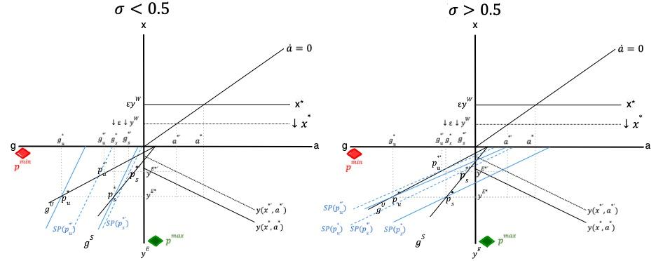
To see the tensions that the green transition and the external constraint entail, assume that the growth rate of exports falls as part of the world economy converging to a zero-carbon economy. As mentioned before, this could take the form of either a de-growth process, represented by a fall in ���� ���� , or a change in production and consumption patterns, resulting in a drop of ���� The impact of such a scenario is represented in Figure 2 where, as before, the right panel assumes a social preference of income over the environment when defining prosperity, and the left panel illustrates the opposite case

First, there is a downward shift in the ���� ∗curve of the top quadrant, implying a tighter balance of payments constraint. This, in turn, shifts the ����(���� ∗ , ����∗ ) schedule upwards in the bottom-right panel, implying a reduction in the long-run growth rate of domestic demand and, consequently, of income

���� ���� ∗ . Note that ���� ���� ∗ < ���� ���� ∗ , i.e., the economic dimension of prosperity is negatively affected permanently. This lower long-run income growth rate entails a lower growth of production, which, given the structural parameters of the economy, is associated with lower growth of greenhouse gas emissions. Note that this will be the case regardless the economy’s productive structure is more or less environmentally sustainable, i.e., whether pollution is defined by the ���� ���� or the �������� lines. The equilibrium prosperity under this new scenario of global green transition would be �������� ∗ ´ if the emissions function is ���� ���� , and �������� ∗ if the emissions function is �������� , with the corresponding growth rates of pollution being �������� ∗ ´ and �������� ∗ , respectively.

Suppose the measure of prosperity gives more weight to income. In that case, the overall effect on the growth rate of prosperity will be negative (�������� ∗ ´ and �������� ∗ are located in a more leftward situated SP curve in the right figure). The opposite will happen if society weighs more on environmental sustainability. In this case, the new growth rates of prosperity are found in a more rightward SP curves, as shown in the left panel. The main conclusions drawn from the figure are the following. First, as happened before, prosperity in �������� ∗ ´ is higher than in �������� ∗ ´ because income growth is the same while pollution is lower. This result is independent on the societal preferences regarding the material and environmental dimensions of prosperity Second, if the rest of the world transitions toward a zerocarbon economy, the long-run equilibrium income growth rate will decrease, but so will pollution. This may lead to higher or lower prosperity growth rates depending on society’s preferences, but it should be borne in mind that even when ���� < 0 5 and prosperity increases, the economic implications of the situation described in the scenario would go against the need of resolving the region’s most pressing pending tasks.

Source: self-elaborated

4. Closure 2: Carbon Neutrality

In the cases analyzed so far no commitment of the country is assumed regarding achieving carbon neutrality at a specific point in the future. The green transition scenario examined in that case consisted of the consequences the domestic economy would face should the rest of the world embark on a process like this. We now analyze the case where the country deliberately transitions toward a zero-carbon productive structure. Such a scenario would imply that in the long run, ���� = 0 From equation (5) it can be seen that for that to happen something else would have to adjust, i.e., be determined endogenously.

To begin with, let us assume a static productive structure implying fixed values for ����, ���� , �������� and �������� In this case, it is either exports or domestic demand that have to adjust to the carbon neutrality goal. Since the latter are already defined such that the economy's growth rate is consistent with the balance of payments equilibrium, it is the growth rate of exports the adjustment variable. Let us call ���� the speed of adjustment of this “green transition”, i.e., how fast the rate of growth of exports adjusts to the discrepancy between the country’s carbon sinks capacity to absorb greenhouse gases from the atmosphere (which is relatively constant) and the economy’s emissions resulting from production.

Recalling the dynamic equation for the growth rate of autonomous expenditures (3) the following system can be defined:

Given that the trace of the Jacobian is negative the first stability condition is satisfied. The second stability condition requires that the determinant is positive. Given the system's structure, this requires that 1 ���� > ���� According to the World Bank, in 2021 the average ���� for Latin American countries hit a historical maximum, reaching 0.276 (the historical average for the period 1960-2021 is 0.2). The various estimates that have been carried out to measure ���� values range between 1 and 3, implying that

5. Therefore, it is plausible that the system is stable. The equilibrium values for the growth rates of exports and autonomous demand are given by:

Setting carbon neutrality as a binding constraint implies that all equilibrium values of income will fulfill this environmental condition. This implies that the environmental dimension of prosperity growth will not only be the same for all equilibria but also take the value ���� = 0. In other words, the different prosperity levels associated with different scenarios will be entirely given by the differences in income.

Figure 3 shows the dynamics of the growth rates of exports and autonomous demand when long-run carbon neutrality is imposed. As in the previous closure, the ���� = 0 locus is upward sloping because as the growth rate of exports is higher, the balance of payments equilibrium growth rate increases allowing domestic demand to grow faster Now, the ���� = 0 locus is no longer independent of the rest of the system's variables. In line with equation 7, it is downward sloping because the higher the growth rate of domestic demand, the lower the growth rate of exports must be to maintain carbon neutrality. The intercept of the exports growth rate function is no longer given by the Thirlwall’s law parameters ���� and ���� ∗ , but by the country’s carbon sinks’ absorption capacity growth rate ����, the share of exports in aggregate demand ����1 and exports’ GHG intensity relative to the economy’s GHG intensity, ���� �������� For realistic values of the parameters is will be the case that �������� ∗ > �������� ����1 �������� , implying that that intercept of the export growth function will be lower in the carbon neutrality scenario than in the cases where there is no self-imposed carbon neutrality. This is intuitive, as carbon neutrality would limit the growth of exports to the balance between their carbon intensity and the economy’s carbon sinks absorption capacity. Far from implying that the relaxation of the external constraint, these changes in the exports growth function make it even more binding, as the country would limit itself to export to the point consistent with carbon neutrality, even if the rest of the world’s demand exceeds that threshold.

Given ���� = 0, we no longer have the different possible ���� curves in the ���� ���� ���� space. Therefore, the ���� = 0 function will overlap with the axis, as shown with the green line next to the ���� ���� axis The fact that there is only one greenhouse gases emission function does not imply that a single productive structure is allowed for (the parameters ����, ���� , �������� , �������� can still take different values) – instead, it is imposed that regardless the values of the parameters exports will always adjust to achieve carbon neutrality in the long-run. As shown in equation 7, the economy's structure as reflected by the parameters will determine the dynamics of the convergence to the long-run equilibrium characterized by carbon neutrality.

Since all the possible equilibria in this scenario share the feature ���� = 0, prosperity is determined entirely by the growth of income ���� ���� Consequently, the level curves of the prosperity function will also overlap with the ���� ���� axis, as shown with the blue line next to (it should actually be overlapping, but for illustrative purposes, it is plotted slightly to the left). Given ���� = 0 and ���� ���� ∗ , the prosperity growth will be given by the subjective parameter ����. A society with a preference for environmental sustainability over income would have an equilibrium prosperity index like ��������2 ∗ , consistent with the long-run equilibrium (���� ���� , �������� ∗ = 0). A country weighing more on the income dimension would find that the same long-run equilibrium combination of income growth and carbon neutrality is associated with a lower level of prosperity, as ��������1 ∗ The higher the weight of the economic dimension on the notion of prosperity, the stronger the trade-off between carbon neutrality and socio-economic well-being will be. This is likely to be the case in South American countries, for which a notion of prosperity where a sustained increase in income levels is not prioritized seems to be an unaffordable luxury. The green transition dilemma, therefore, appears again as a dead end for most South American countries

Compared to the prosperity growth rates obtained in the previous closures the ones generated in the carbon neutrality scenario will be far from ���������������� However, it is not evident that carbon-neutralityconsistent prosperity levels will be close to what countries need to provide their population with a decent life. As shown in Figure 3 and the expressions for ���� ∗ and ����∗ , the long-run equilibrium income growth rate in the zero-carbon scenario is strongly determined by the structural parameters. A higher intercept of the ���� = 0 schedule would lead to a higher ���� ∗ , and so would a smaller slope. Similarly, a smaller slope of the ���� = 0 schedule would also bring about higher ���� ∗ and ����∗ , leading to prosperity growth rates closer to ���������������� . Where each economy locates itself in the ���� ���� ���� space and how close it would be from ���������������� under each closure and scenario is an empirical question that requires giving the parameters the values representing the corresponding productive structure