Forecasting Steel Prices Using ARIMAX Model: A Case Study of Turkey

(a) and PACF (b), source: own estimations

Due to the steep fall of ACF to zero and a significant positive spike in the first and negative spikes on second and third lags of the PACF diagram, using George Box & Jenkins (1976) guideline, initially, ARIMA (1, 1, 2) and (0,1,2) seems to be possible outcomes for the model. Therefore, further investigation is needed to generate the best model, according to BIC. After several tries to minimize BIC, it is revealed that the best model is ARIMA (0,1,2). The result of ARIMA coefficients estimation is showed in Table 2.

Notes:

As seen from the results, MA coefficients are significant and also satisfies the condition of stationarity and invertibility

,��2 <1,��2 ��1 <1,��1 +��2 <1 ) as described in (George Box & Jenkins, 1976).

The Ljung-Box test is used widely for testing randomness and the existence of serial correlation in the error series. It is a comprehensive statistical test for a set of autocorrelation lags instead of one to define that they are significantly different from zero, and thus they are not random. The null hypothesis for this test is that the series is not autocorrelated, and the alternate hypothesis is auto-correlated. In our model, due to the insignificant p-value, we can conclude that errors are not auto-correlated. Also, the Durbin-Watson (DW) test, which is used to detect serial correlation in the first lag, is almost 2.00, which shows no evidence of positive or negative serial correlation where it is consistent with the result of the Ljung-Box test.

For entering explanatory variables into the ARIMA system, an equation with explanatory variables of LnSCP, LnORP and, LnOIP with correspondent lags on the right side, and dependent variable LnSTP on the left side has to be formed. After then, regarding remaining patterns in residuals, the ARIMA process fitted to the residuals. All the system is optimized with consideration to BIC minimization. The results for the ARIMAX process are demonstrated in Table 3.

Table3

ModelEstimationResults

Notes:DW:Durbin-Watsonstatistics

Forecasting Steel Prices Using ARIMAX Model: A Case Study of Turkey

After the correct lags are selected for explanatory variables, it is found that ARIMA (1,1,0) is the best model for residuals. The condition for stationarity and invertibility for AR(1) is fulfilled ( 1<��1 <1 ). The specified model has the lowest BIC among tested models, and regarding the DW and Ljung-Box test, there is no serial correlation in the residuals. As seen from the estimation results, the LnSCP and LnOIP only take effect after lags 4 and 3, respectively. By contrast, LnOIP has an instantaneous effect on LnSTP.

3.3 Forecast Results

In order to make an out-of-sample forecast in the multivariate ARIMAX model, initially, the forecasted values of the explanatory variables have to be defined. For this aim, the ARIMA model is used for forecasting each variable separately. Regarding the ARIMA methodology, ARIMA (1,1,1), (0,1,1) and (0,1,1) are utilized for LnSCP, LnORP and, LnOIP for forecasting July 2019 until December 2019. The results of the out-of-sample forecast for ARIMA (0,1,2) and ARIMAX (1,1,0) models are represented in Table 4.

Table 4 Forecast precision for LnSTP

2.0279304% 3.034979%

Notes: MAPE: Mean Absolute Percentage Error

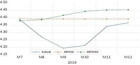
In this study for comparing the forecast results, Mean Absolute Percentage Error (MAPE) is used. Hyndman & Koehler (2006) stated that MAPE has clear lines and can be helpful in the case of positive and comparatively large to zero variables. The forecast results visualization of two models is shown in Fig 2.

2. Forecast Results for ARIMA and ARIMAX, source: own estimations IV. Discussion

As observed from the results, the univariate ARIMA model outperforms the multivariate ARIMA with explanatory variables. The MAPE is lower about a half in ARIMA comparing to the ARIMAX model in the 6-month forecast horizon. While the ARIMAX model is better fitted to data in aspects of R-Square and BIC, it is not performing better than the univariate ARIMA model. The result is consistent with Peter & Silvia's (2012) findings, which compare ARIMA and ARIMAX for Gross Domestic Production (GDP) forecast. Also, the study by Kongcharoen & Kruangpradit (2013) showed mixed results for export rates between the two models, which in some cases, ARIMA yields better results than ARIMAX.

While rationally, the ARIMAX model is expected to forecast better than ARIMA due to the inclusion of the explanatory variables, it offers worse results. One explanation of this situation can be the necessity of forecasting each explanatory variable separately with univariate models to use in the ARIMAX system, which in turn adds more uncertainty to the system. Another reason might be the forecast horizon that can be effective owning to the long-run relationships between the explanatory variables.

V. Conclusion

The current study aims to forecast flat steel prices by using the ARIMAX model and compares the performance with the ARIMA model as a benchmark. In contrast with the role of explanatory variables to improve the forecast accuracy, the findings of the study prove that the ARIMA model’s out-of-sample forecast results outperform the ARIMAX model. However, the model fit statistics in the ARIMAX model is better than the ARIMA model. Since the ARIMAX model uses forecasted values for explanatory variables by univariate models, the iterative nature of univariate models adds more

Forecasting Steel Prices Using ARIMAX Model: A Case Study of Turkey uncertainty to the system, which may lead to worse performance. For this problem, more complex models that utilize past values of explanatory variables like Vector Autoregressive (VAR) and Vector Error Correction (VEC) can be used.

References

[1] Worldsteel Association. (2019). WORLD STEEL IN FIGURES 2019. Retrieved from https://www.worldsteel.org/en/dam/jcr:96d7a585-e6b2-4d63-b9434cd9ab621a91/World%2520Steel%2520in%2520Figures%25202019.pdf

[2] ITA. (2019). Global Steel Report. Retrieved from https://www.trade.gov/steel/pdfs/global-monitor-report2018.pdf

[3] ERDEMIR. (2019). 2019 12 Months Investor Presentation.

[4] Blecker, R. A. (1989). Markup Pricing, Import Competition, and the Decline of the American Steel Industry. Journal of Post Keynesian Economics, 12(1), 70–87. https://doi.org/10.1080/01603477.1989.11489781

[5] Blonigen, B., Liebman, B., & Wilson, W. (2007). Trade policy and market power: The case of the us steel industry. In NBER Working Paper No. 13671. Retrieved from http://www.nber.org/papers/w13671

[6] Grossman, G. M. (1986). IMPORTS AS A CAUSE OF INJURY: THE CASE OF THE U.S. STEEL INDUSTRY. Cambridge.

[7] Liebman, B. H. (2006). Safeguards, China, and the price of steel. Review of World Economics, 142(2), 354–373. https://doi.org/10.1007/s10290-006-0071-y

[8] Mancke, R. (1968). The Determinants of Steel Prices in the U . S .: 1947-65. The Journal of Industrial Economics, 16(2), 147–160.

[9] Richardson, P. K. (1999). EC steel prices and imports Impact of imports from Eastern Europe. Journal of Product & Brand Management, 8(5), 443–454. https://doi.org/10.1108/10610429910296046 https://doi.org/10.1134/S1075700711030105

[10] Malanichev, A. G., & Vorobyev, P. V. (2011). Forecast of global steel prices. Studies on Russian Economic Development, 22(3), 304–311.

[11] Kahraman, E., & Unal, G. (2012). Steel Price Modelling With Levy Process. International Journal of Economics and Finance Studies, 4(1), 101–110.

[12] Wu, B., & Zhu, Q. (2012). Week-ahead price forecasting for steel market based on RBF NN and ASW. ICSESS 2012 - Proceedings of 2012 IEEE 3rd International Conference on Software Engineering and Service Science, 3, 729–732. https://doi.org/10.1109/ICSESS.2012.6269570

[13] Liu, Z., Wang, Y., Zhu, S., & Zhang, B. (2014). Steel Prices Index Prediction in China Based on BP Neural Network. 4th International Conference on Logistics, Informatics and Service Science, 603–608. https://doi.org/10.1007/978-3-662-43871-8

[14] Ming-Tao Chou, Ya - Ling Yang, S.-C. C. (2012). Review of Economics & Finance A Study of the Dynamic Relationship between Crude Oil Price. Better Advances Press, Canada in Its Journal Review of Economics & Finance., 2(May), 30–42. Retrieved from http://webcache.googleusercontent.com/search?q=cache:KFeezAJrHsQJ:https://ideas.repec.org/a/bap/jour nl/120203.html+&cd=1&hl=en&ct=clnk&gl=uk

[15] Chou, M. T. (2016). Dynamic economic relations among steel price indices. Journal of Marine Science and Technology (Taiwan), 23(5), 919–925. https://doi.org/10.6119/JMST-016-0504-1

[16] Todshki, N. E., & Ranjbaraki, A. (2016). The Impact of Major Macroeconomic Variables on Iran’s Steel Import and Export. Procedia Economics and Finance, 36(16), 390–398. https://doi.org/10.1016/s2212-5671(16)30051-x

[17] George Box, & Jenkins, G. (1976). TIME SERIES ANALYSIS (5th ed.). John Wiley & Sons.