22 minute read
3. From emissions inventory to air quality assessment and forecasting
Air quality assessment entails inferring the air quality at times and locations where observations are insufficient or lacking. In many cases, the assessment is about predicting the spatial distribution of pollutants averaged over time periods on a monthly, seasonal or an annual basis. In these studies, maps of pollutant concentrations enable the identification of hot zones, and when coupled with population patterns, provide valuable insights about exposure. In addition, some of the modelling tools described below allow for exploring “what-if” scenarios, thus providing an effective framework for mitigation, informing policy makers, and planning.
An especially important form of air quality assessment is air quality forecasting, which entails prediction of future air quality, starting with a set of initial conditions. An accurate and reliable air quality forecast is a key component of air quality management system that (i) provides effective health alerts to the vulnerable population, (ii) supplements traditional emission control programs, (iii) empowers operational planning, and (iv) enables more effective emergency response. Example of governments control measures include limiting traffic circulation and temporarily shutting down factories and plants. Improving air quality forecasting also involves prediction over a longer period of time, which allows for better preparation for extreme events.
This chapter is intended to provide a basic understanding of pollution dispersion assessment and forecasting tools to help countries make informed choices as to which air quality assessment tool is most suitable to answer a given question. After introducing the concepts of air quality assessment and forecasting, the importance of air quality measurements is discussed.
This is followed by the presentation of the different types of data, including on emissions, required by air quality modelling tools. Then, different approaches to air quality forecasting are then presented, followed by the showcasing of two methods for assessment and forecasting: land use regression (LUR), and physically-based numerical dispersion. LUR is a widely used statistical method that correlates observations with land use data to infer the spatial distribution of the pollutant concentration. The physically-based numerical dispersion method is the tool of choice for predicting the spatio-temporal concentration distribution when emissions, geometrical, and meteorological data are available.
A more detailed and encompassing exposition of air quality assessment and forecasting approaches and the associated modelling tools is presented in a separate guidebook,2 where the different methods are compared in terms of their applicability, data requirements, spatio-temporal resolution, and computational cost.
3.1 Air quality measurements
Availability of periodic air quality measurements that are adequately spaced is key to improving the accuracy of air quality assessment and forecasts. Air quality measurements refer mainly to ground or near-ground observations of ambient concentrations of pollutants. Air quality measurements also improve the ability of modelling tools to identify pollutant sources (where and when), quantify the contribution of different source types (e.g. traffic, industry), explore what-if scenarios, assess mitigation strategies and plan for the future, and uncover the dominant patterns and the underlying dynamics. Measurements over long periods of time are necessary for climate forecasts such as predictions of the ozone layer thickness and spread, and of temperature and sea level rise.
3.2 Data requirements for air quality assessment and forecasting
Air quality assessment involves spatio-temporal modelling of the dispersion of pollutants. These advanced computer models predict the distribution of pollutant concentrations in space and time. The choice of modelling approach and the types of data required are strongly dependent on the desired spatial and temporal resolutions. The data can be arranged in the following categories: (a) meteorological, (b) emissions, (c) geometric (buildings), (d) geographic, (e) observations (e.g. air quality measurements), and (f) land use.
Air quality assessment requires meteorological data. The starting point of any air quality forecasting is a meteorological forecast. The weather forecast predicts the time-dependent thermophysical properties of air that drive and characterize the local transport of pollutants. Thus, the accuracy of the air quality forecast depends, in part, on the reliability of the weather forecast. To produce the most accurate weather forecast possible, the output of several forecasting models is typically combined with local experience and knowledge. The most accurate air quality forecast possible is therefore one that follows a similar approach.
The emission inventory, which is the main subject of this guidebook, is widely used as an input to air quality models. This is especially true for physical models that model the dispersion of the pollutants originating from the emission sources. In these models, the emission inventory is incorporated through specifying the locations of the emission sources and their emission rate as a function of time. Emission sources include residential buildings, industrial buildings, power plants and generators, traffic, agriculture and forest fires. Depending on the scale of the study and the intended spatial resolution, the emission sources can be represented individually (if the study domain is a street canyon) or as area or line sources (if the study domain is a country or larger). Air quality assessment based on statistical modelling tools, such as LUR models, typically employs distances from emission sources or zones of high emissions such as highways or industrial plants.
Air quality assessment and forecasting models also take as input the digitized representation of topography (terrain) in addition to other obstacles such as buildings. The resolution of these representations has to be compatible with the length scale resolved by the model. This length scale is determined, to a large degree, by the domain size.
Air quality ground monitors provide direct measurements of pollutant concentrations at ground level. Ground measurements are commonly taken on a daily or, preferably, on an hourly basis. The spatial distribution of the monitoring stations is key when used by a modelling tool to improve air quality assessment. Pollutants can also be measured using satellites, aircraft and balloons. Other aspects include supporting and training local scientists in data collection, including meta data such as sensor height above the ground, and distance from buildings, roads, and emission sources. To enable regional solutions to be possible, the data has to be shared among the stakeholders.
Some statistical methods such as LUR require land use data. Land use data describe the use of land for various human activities including industrial, agricultural, residential, recreational and other activities.
3.3 Modelling tools for air quality assessment and forecasting
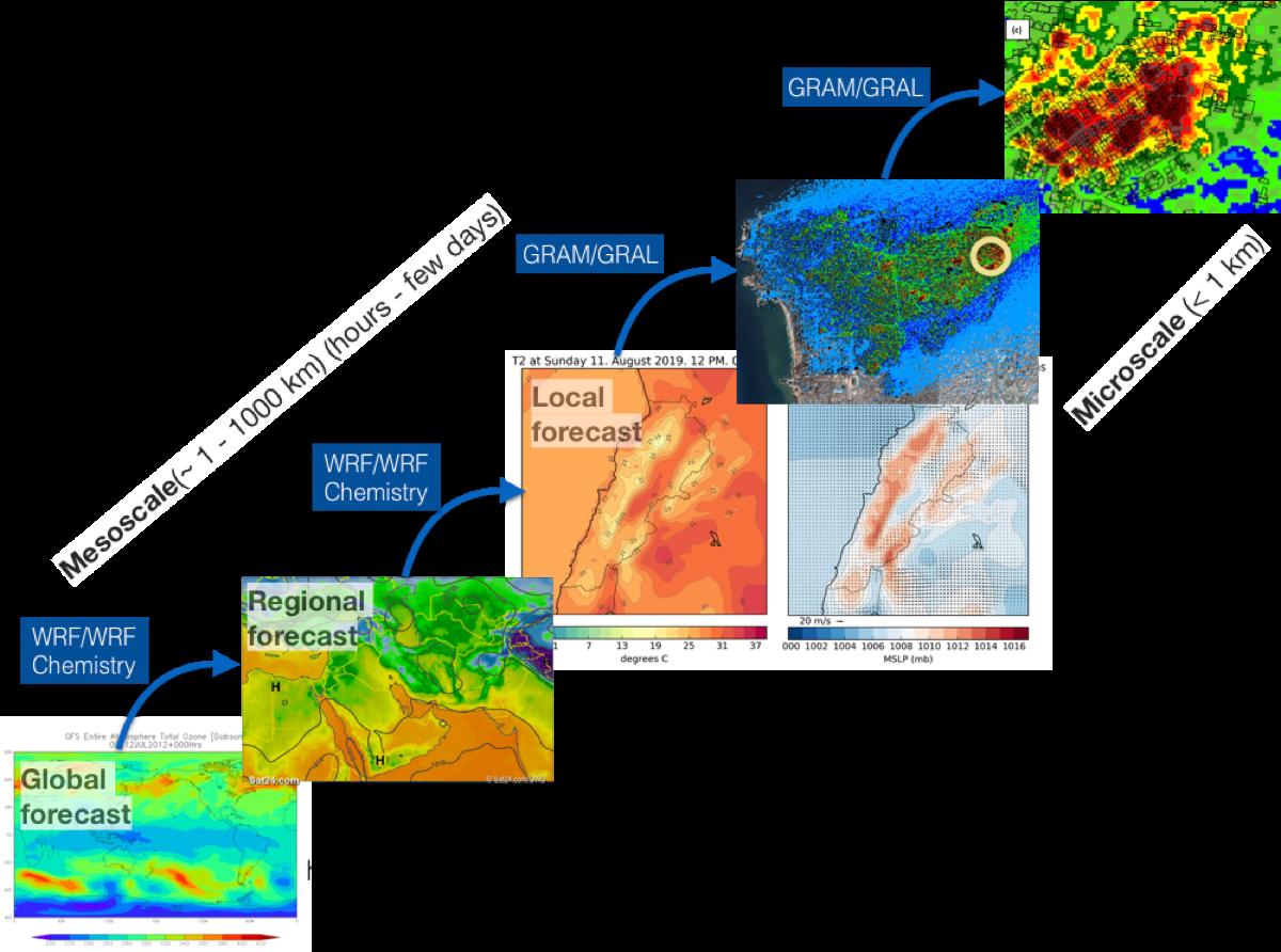
Modelling tools may be categorized based on the length and time scales they resolve. An example of the different meteorological forecasting tools used to resolve different length scales is shown in Figure 1
A global forecast, such the Global Forecast System (GFS) produced by the National Centers for Environmental Prediction (NCEP), provides weather forecasts for up to 16 days into the future at a resolution of 28-70 km. Regional and local operational forecasting down to the ~ 1 km scale is carried out using tools such as the Weather Research and Forecasting (WRF) model.3 These tools incorporate the GFS forecasts and numerically model transport based on the governing physical laws, while allowing assimilation of data from observations.
Different techniques of varying complexity have been used for weather and air quality forecasting. Air quality forecasting methods fall into two broad categories: deterministic and probabilistic. While a deterministic forecast predicts a specific event, such as a storm, that will take place at a specific time and location, a probabilistic forecast yields an ensemble of possible events each with a quantifiable likelihood (or uncertainty). Given the numerous uncertainties and in some cases the limitations in observations, probabilistic methods are increasingly used by researchers to quantify the uncertainties associated with the predictions.
These uncertainties arise from lack of full and accurate knowledge of local weather conditions, measurements (e.g. local pollution emissions and concentrations) and boundary conditions (e.g. long-range transport 4) in addition to model parameters such as the mixing coefficient. Models for assessing and forecasting air quality can be alternatively divided into three categories: potential forecasting, physically-based numerical methods and statistical methods.
Physically-based refers to methods that numerically solve equations governing the conservation of mass and momentum. Statistical methods, on the other hand, rely on tools such as linear regression (LR), principal component analysis (PCA), statistical trend analysis, neural networks, and more recently artificial neural networks and deep learning. Physically-based numerical models can be deterministic in the sense that they yield a fixed output for a given input, or stochastic in the sense that they yield a probabilistic ensemble of solutions which arise from uncertainty in model parameters.
3 https://www.mmm.ucar.edu/weather-research-and-forecasting-model
4 Concentrations and emissions at distant sources and their transport: advection, mixing, and chemistry.
3.4 Forecasting methods
As mentioned earlier, air quality forecasting is a type of assessment that predicts future air quality, starting with a set of initial conditions. Three categories of air quality forecasting approaches are presented briefly below.
3.4.1 Potential forecasting
Potential forecasting is a qualitative method that relies on meteorological conditions such as atmospheric dilution and ventilation capacity to issue a warning when these conditions are expected to be similar to those associated with serious pollution (Tong and Wan, 2001).
Increasing the reliability of these forecasts involves collecting data on pollution levels for different meteorological conditions over many years. The potential forecasting method is a good predictor when weather patterns are similar to those of previous years.
If the patterns are different, for example due to global warming, the accuracy of the forecast will suffer. Predicting air quality using this method is based on associating elevated pollution levels with specific meteorological conditions. This requires employing sophisticated weather typing schemes for identifying recurrent weather patterns accompanying high pollution levels. Potential forecasting has the advantage of being relatively simple and cost-effective. Since it does not rely on pollution measurements or emissions, the potential method has the disadvantage of being qualitative and less accurate than the quantitative methods discussed below.
3.4.2 Statistical methods
Statistical forecasting methods range from classical statistical methods such as LR to more recent methods of artificial intelligence (AI) and machine learning (Kaya & Gündüz Öğüdücü, 2020). These methods are capable of short and long-short (24 hrs) range prediction and enable the prediction of several pollutants from knowledge of one pollutant.
Statistical methods include linear and nonlinear supervised learning methods and are easily distinguishable from deterministic models by their randomness properties, which arise from treating the modelling and measurement errors respectively as system and observation noise obeying certain probability distributions (Sawaragi et al., 1977). Machine learning approaches from statistical models have proved their superiority to deterministic models in many air pollution studies (Kaya & Gündüz Öğüdücü, 2020). They have also been shown to be superior to traditional statistical methods such as multiple regression, autoregressive models and classification and regression trees (Yi & Prybutok, 1996; Chaloulakou et al., 2003).
The association between pollutant levels and meteorological and aerometric variables can be quantified by analyzing historical data sets using standard statistical analysis packages. Methods such as LR and PCA (Bai et al., 2018) enable estimation of the model parameters. An example of a multivariate analysis, which employs correlation analysis, PCA, and cluster analysis is presented in Núñez-Alonso et al. (2019) to interpret and model air pollution data (PM10, NOₓ, O3) collected from 22 stations in the city of Madrid during 2010-2017. Statistical trend analyses, for instance using the Mann Knedall and Sen’s slope estimator approaches, enable the prediction of pollutants (CO, NO2, SO2, PM2 5 and PM10) in Varanasi, India, when combined with the autoregressive integrated moving average model (ARIMA), as presented in Jaiswal (2018).
A real-time pollution forecast with early warning ability to predict pollutants (CO, NO, PM2 5, NO2) in three different locations in Valencia, Spain, is presented in Ochando (2015). The regression models in Ochando (2015) are trained using (i) meteorological features (temperature, pressure, relative humidity, wind speed, and rain), (ii) calendar features (year, month, day in month, day in week, and hour), (iii) traffic intensity features (traffic levels in surrounding stations) and (iv) pollution features (pollution levels in target stations 3 and 24 hours earlier). Classification and regression tree (CART) statistical models use meteorological or air quality variables that are strongly correlated with ambient pollution levels to predict future air quality based on the current air quality and the meteorological forecast. An example is presented in Yoo et al. (2018).
An example of a recent air quality forecasting model that employs deep learning in presented in Kaya & Gündüz Öğüdücü (2020). The deep flexible sequential (DFS) learning model employs a dataset that includes hourly pollution and meteorological data from four stations in Istanbul, Turkey between 2014 and 2018, in addition to traffic data. The flexibility in the model makes it applicable to time-series data. This is in contrast to traditional artificial neural network models (ANN) that do not forecast with sequential information (Kaya & Gündüz Öğüdücü, 2020).
3.4.3 Physically-based numerical dispersion models
These methods quantify the relationship between pollutant concentrations and emission sources, meteorological processes, and physico-chemical changes. These methods are deterministic when the model parameters are deterministic so that the output is fixed for a given fixed input.
Examples of physically-based numerical dispersion methods are shown in Figure 1 for different scales. Another commonly used deterministic model that is widely used in Asia is the community multi-scale air quality (CMAQ) modelling system (Bai et al., 2018; Tong & Wan, 2001).
Also of note are recent efforts towards hybrid approaches that combine statistical analysis with physically-based numerical prediction. An example is the method presented in Chen et al. (2015), which was used to forecast the daily PM10 concentrations in Beijing, China, from January 1 to December 30, 2013. Air quality data from 12 stations in Beijing for the period 2000-2011 were used in the study.
3.5 Assessment methods
To showcase statistical and physically-based numerical methods for air quality assessment and forecasting, we discuss below two of the most widely used air-quality assessment methods in urban environments. The LUR model for spatial assessment and the Lagrangian dispersion computational model for spatio-temporal assessment. Note that the Lagrangian model can be used for air quality forecasting.
3.5.1 Land Use Regression models
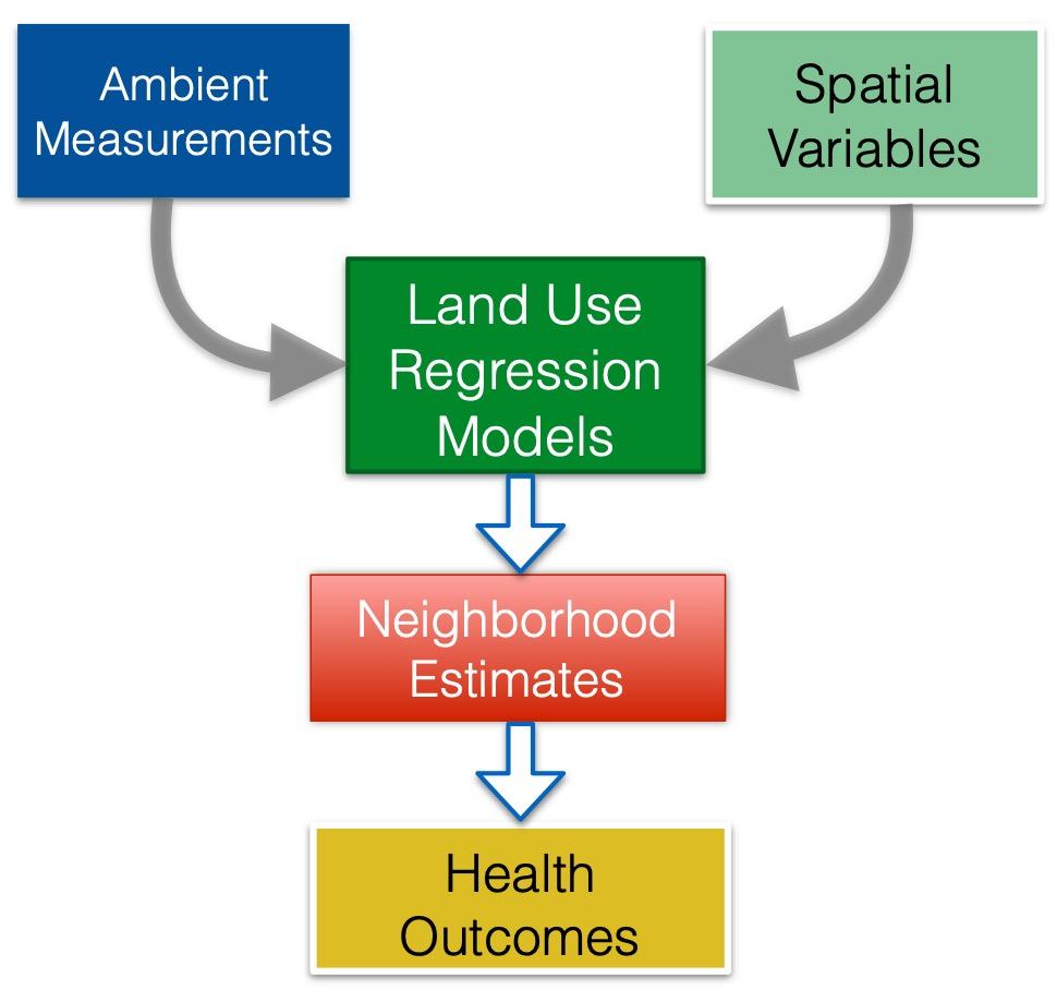
LUR is a widely used method to estimate individual exposure to ambient air pollution in epidemiological studies. LUR has been successfully applied to model annual mean concentrations of NO2, NOₓ, PM2 5, black carbon, the soot content of PM2 5 and VOCs in different settings. The performance of the method in urban areas is typically better or equivalent to geo-statistical methods (such as kriging) and dispersion models. LUR combines monitoring of air pollution and development of stochastic models using GIS-based predictor variables. A schematic is shown in Figure 2. Monitoring campaigns are typically conducted spatially at about 20-100 locations spread over the study area, and temporally via 1-4 surveys of 1-2 weeks duration.
The GIS-based predictor variables needed in the stochastic models include traffic representations, population density, land use, physical geography (e.g. altitude) and climate. A typical land use multivariate LR model starts with an initial pool of 30-80 potential predictors (variables). Reduction in the number of predictors is realized by eliminating variables that are highly correlated with other variables or due to lack of interpretability. Typically, a significantly smaller number of variables end up being used in the model.
Establishing a monitoring programme involves deciding whether to use routine or purposefully designed networks for the ambient measurements. While using routine (pre-existing) networks is significantly less costly, it does not offer the possibility of selecting the locations of the monitoring stations. With purposefully designed networks, the number and distribution of monitoring sites is customized for the domain of interest, in addition to temporal aspects including the number, dates, and durations of the campaigns.
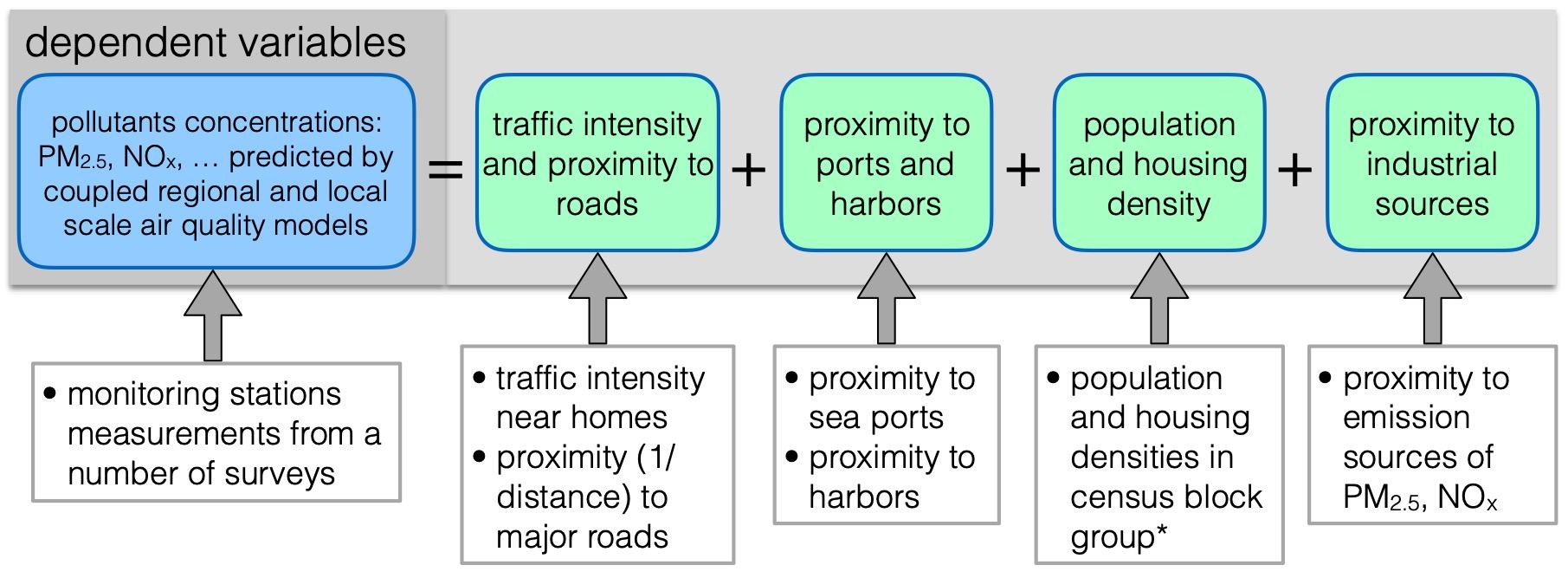
Figure 3 lists some commonly used predictor variables, which fall into the following categories: (i) traffic, (ii) population or address density, (iii) land use, (iv) altitude and topography, (v) meteorology, and (vi) location. Most of these variables are accessible within a GIS framework. Attention should be paid to the uncertainty associated with these variables arising from potential problems with geographic data sets such as accessibility, completeness and precision. It should be noted that the technology is advancing at such rate that many previously encountered issues may have been resolved.
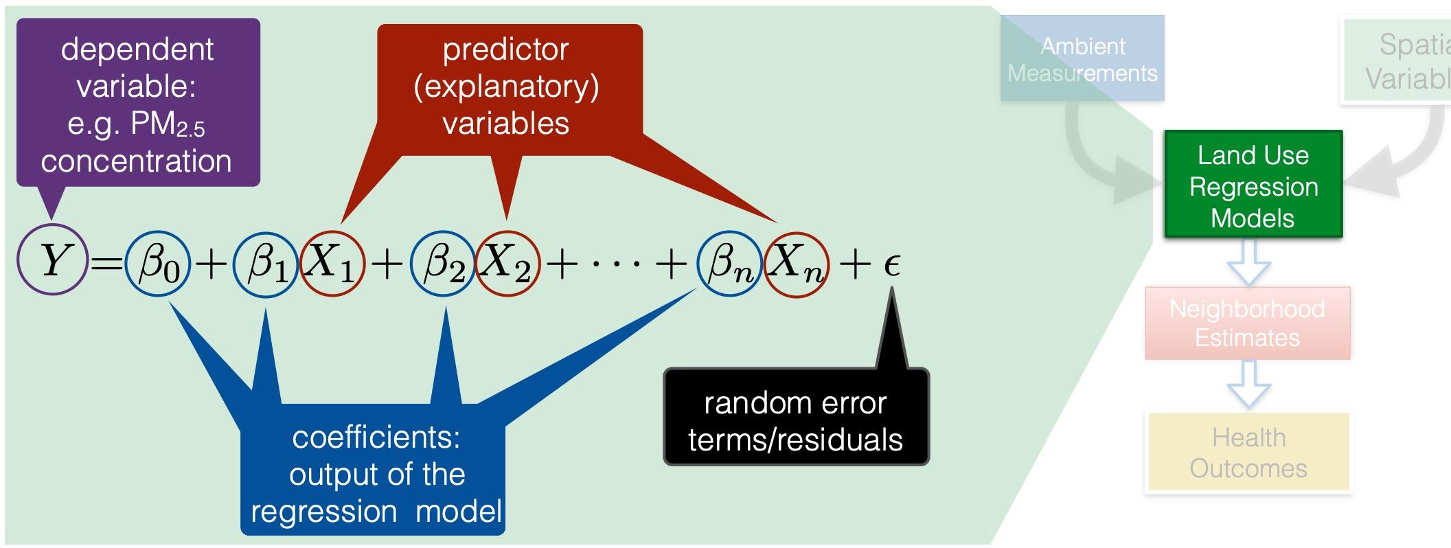
Commonly, standard LR techniques are used to develop the prediction models. A mathematical representation is shown in Figure 4. The coefficient βi associated with independent variable Xi is characterized by a p-value, which measures the probability for the coefficient. The closer the p-value is to zero, the more important is the predictor variable in the LUR model. The overall model performance is quantified using the R-squared value, which measures how well, over a range 0-100, the model fits the observations. For a perfect fit, R2=1.
A key advantage of LUR models is that they are capable of capturing small-scale variability in community health studies. Additionally, they are less resource intensive than other methods, as land use data is widely available. LUR models still face several challenges.
They require accurate monitoring data at a large number of sites. Their lack of ability to connect specific sources of emissions to concentrations hinders their potential for developing pollution control strategies. Their application in regions where a significant portion of the population lives in high-rise buildings may seriously misclassify exposure, especially in high-rise buildings near major roads. LUR models often employ circular buffer zones. This imposes some level of isotropy, which may not be representative. When used in health studies, LUR models are not transferable from one region to another. They also do not address multi-pollutant aspects of air pollution. They also lack the fine scale temporal resolution needed for short-term exposure studies. In addition, they estimate outdoor air pollution as opposed to indoor or personal. Current and future research efforts are focused on tackling some of these challenges, in addition to the incorporation of some meteorological conditions and emission data into the pool of predictor variables.
3.5.2 Lagrangian dispersion computational models
As opposed to statistical methods, dispersion models rely on physically-based spatio-temporal5 simulation of the transport of mass, momentum, energy, and chemical species.
Transport of pollutants originating from the emission sources is carried out by numerically solving the associated transport equation, which requires knowledge of the meteorological conditions. In the absence of chemical reactions, this transport is governed by advection and diffusion (mixing). Accounting for the advection of pollutant particles requires knowledge of the local velocity, while accounting for mixing requires knowledge of the local turbulent mixing diffusivity, which in turn depends on the velocity field and other thermophysical properties.
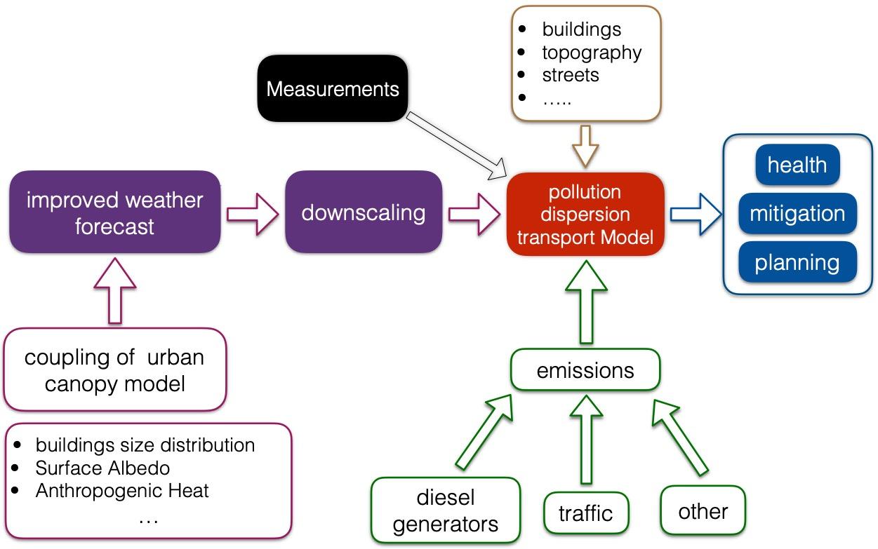
In addition to accurate representation of the spatio-temporal meteorological variables, the locations, emissions rates, and schedules of all the emission sources must be reliably measured. Figure 5 shows how all the components that make up a dispersion model come into play.
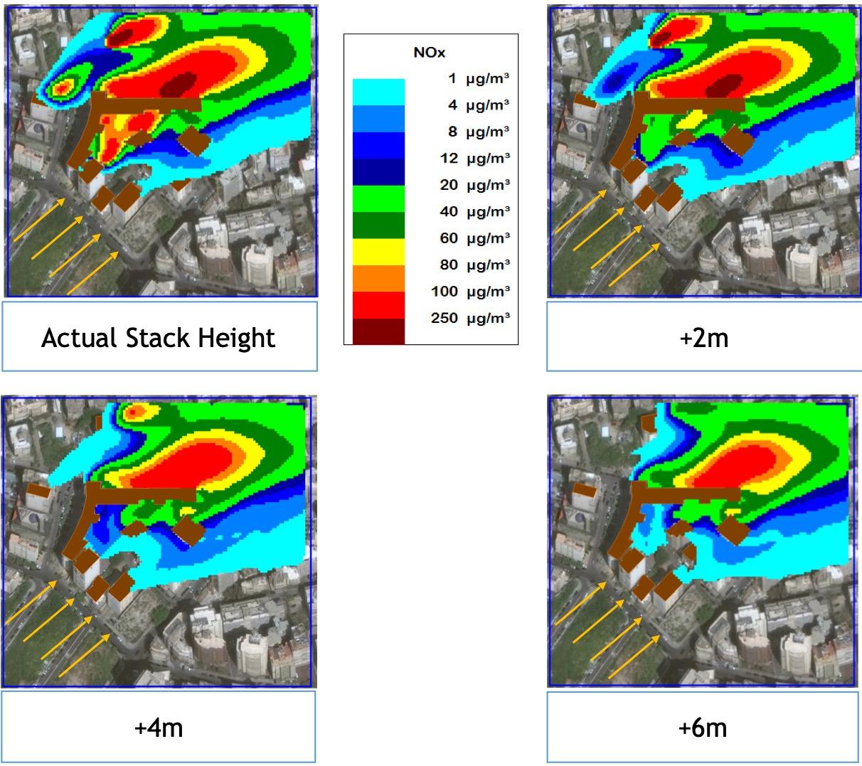
Dispersion models predict the time-varying three-dimensional spatial distribution of pollutant concentration in a user-controlled simulation environment. As such, they enable investigation of what-if scenarios and exploration of mitigation strategies. For example, all of the following questions can be answered using dispersion models: What is the exposure of all those living on the 8th floor? How will elevating all the emission stacks by 5 m impact the ground pollution levels under different weather conditions? In the next five years, when 1,000 buildings will be torn down and 1,500 erected, how can exposure be reduced? An example is shown in Figure 6, where the impact of extending the stack height of six diesel generators on the NOₓ colormaps at 30 m above ground is explored as a way to reduce residents’ exposure in a neighborhood in Beirut.
Three-dimensional dispersion computational models may be either Lagrangian or Eulerian. While Eulerian models solve the transport equations on a grid, Lagrangian models follows particles in time as they are advected by the velocity field. There are numerous advantages from using Lagrangian models as opposed to Eulerian models. These advantages include not having to deal with the non-linear advection term, which is often dealt with using upwind schemes in Eulerian methods.
While dispersion models have the advantages of predicting the time-varying three-dimensional distribution of pollutant concentrations and enabling exploration of what-if scenarios, they face the challenge of uncertainties that impact the accuracy of their results. These include uncertainties in (i) the emission sources (rates, spatial distribution, schedule), (ii) the downscaled fields of the thermophysical properties (velocity, temperature, etc.), and (iii) the mixing coefficients. These uncertainties can in some cases be reduced by assimilating observations into the dispersion model. Data assimilation and uncertainty quantification have become indispensable tools that transform dispersion modelling into a powerful predictive framework.
3.6 Input data requirements
The LUR method combines monitoring of air pollution with stochastic models using GIS-based predictor variables. Monitoring takes place at 20-100 locations spread over the study area and is temporally limited to 2-4 surveys of typically 1-2 weeks duration each. A list of commonly used predictor variables is presented in Table 1. Note that spatial predictor variables are available in GIS tools such as ARCGIS or QGIS, though these can be improved by taking measurements. Some variables may require additional effort. For traffic, for example, a challenge is the accessibility of traffic intensity data. Traffic counts are typically only available for a small number of streets, mainly for major roads and highways. In the absence of detailed data, traffic models can be used to assign traffic counts to other roads, and in some cities modeled data are available from transport and highway authorities. Alternatively, the length of specific road types can be used.
Predictor variables in LUR models are usually computed for circular zones around each monitoring site, using buffer functions in the GIS. The buffer sizes should be selected to take account of known dispersion patterns. These include impacts of major roads and inner-city area. Concentrations of traffic-related air pollutants decline exponentially with distance from the road. Beyond about 100 m from a major urban road, or 500 m from a major freeway, variability is limited. In street canyons, marked accumulation of air pollution may occur, especially against the windward side of buildings, with the result that concentrations may differ substantially from one side of the road to another. Other aspects of inner-city areas include oxygen-limited formation of NO2 (from NO) in street canyons, and the drop of pollution concentration virtually to background levels behind a row of uninterrupted buildings.
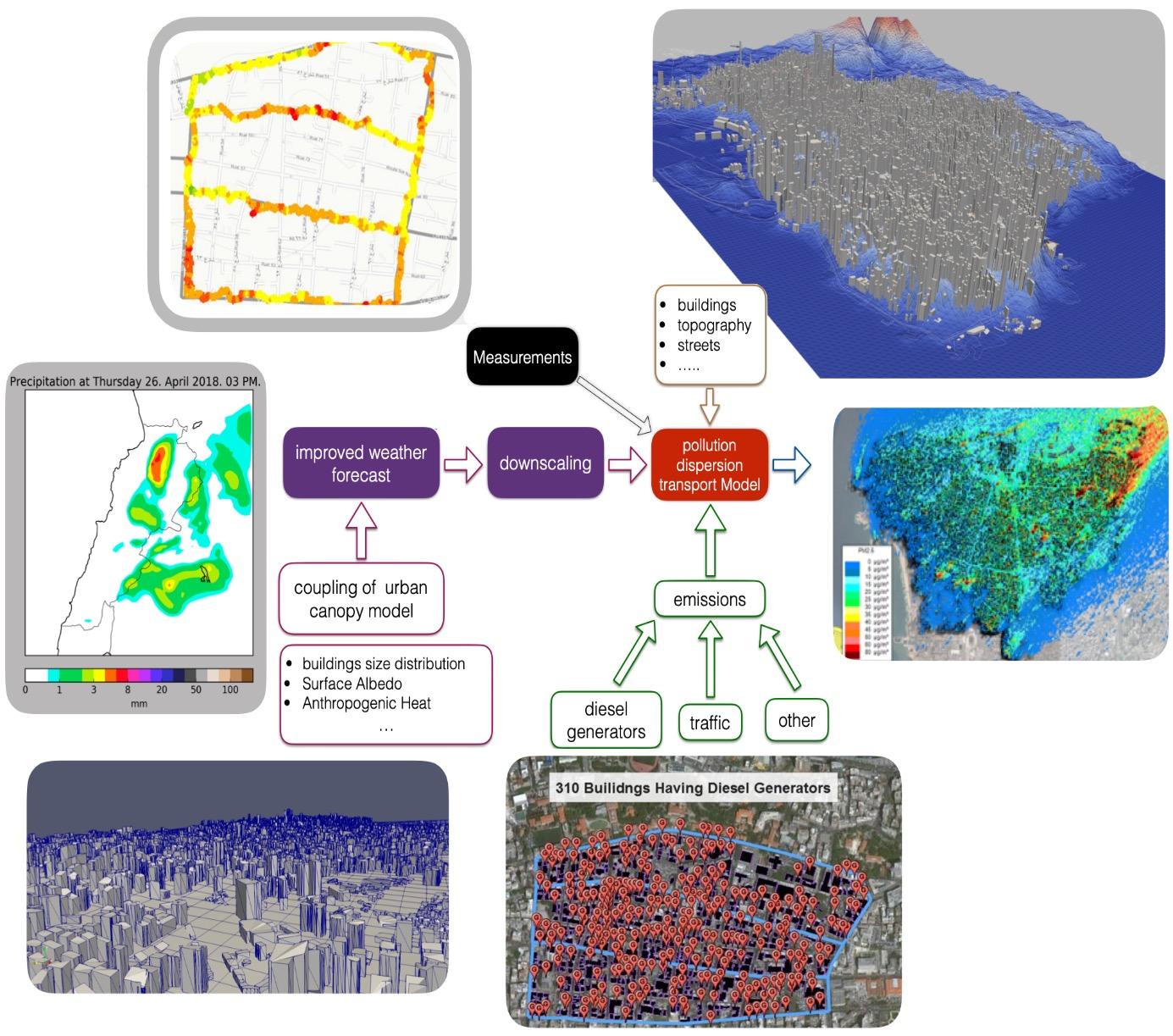
The pollution dispersion transport model takes as an input the digitized representation of the buildings, topography, and streets, as seen in Figure 7 for the case of Beirut city. It also takes as an input the emission sources data and the downscaled fields of velocity and other thermophysical properties such as temperature and density. The time-varying 3D fields of velocity and other thermophysical properties can be obtained using a weather forecast tool. For example, the WRF model can be coupled with an urban canopy model (UCM) to produce more accurate predictions in urban environments. The UCM requires an accurate description of building sizes distribution, surface albedo, and anthropogenic heat.
Modelling pollution dispersion at smaller scales (2-1000 m) requires another round of downscaling of the meteorological mesoscale conditions onto a well resolved domain. Well resolved means that the geometrical representation of the domain must accurately capture all features within the desired resolution. Thus, to model dispersion at the urban canopy scale (2-5 m), the numerical representation of the domain must accurately capture the topography and buildings to within the required resolution.
Category
Predictor variables
Traffic intensity
Percentage traffic jam
Traffic
Number of trucks
Road length
Residential
Non-residential
Land cover
Agriculture Parks
Water bodies
Area of open space
Major roads
Sea
Distance to
Population
Petroleum facilities
Factories
Number of buildings
Population
Household density
Physical geography
Geo
Meteorological
Sampling
Emissions
Altitude
Meteorological region
Climate
Sampling height
Total primary emissions of pollutant
Pollutant emissions from major road vehicle sources
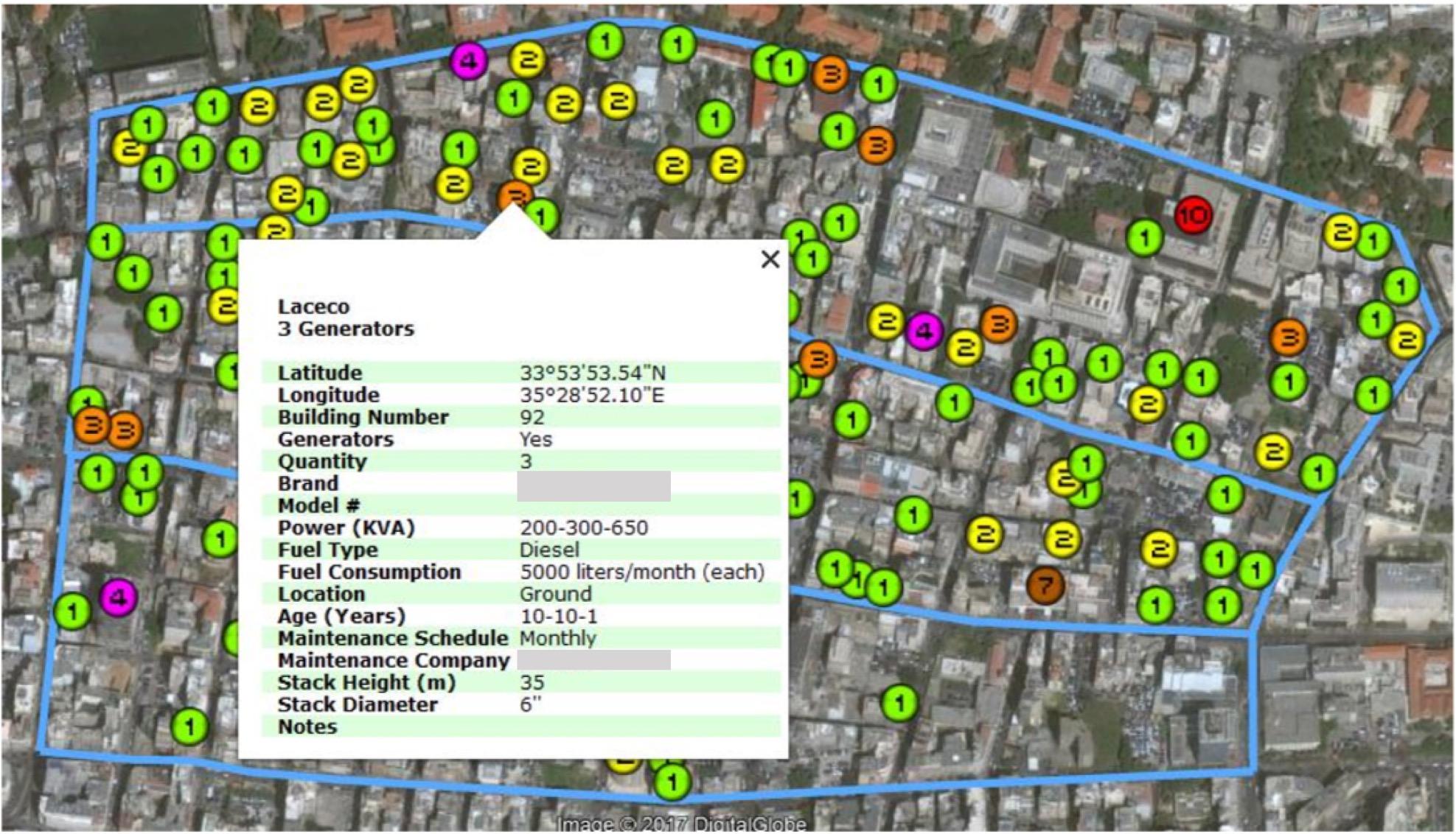
In addition to the downscaled thermophysical fields and the digitized topography, buildings and streets, an accurate emission inventory must be in place for the dispersion model to work. It is recommenced to build the emissions inventory in a GIS environment due to the many ensuing advantages. An example is shown in Figure 8, which shows a sample of the data collected on diesel generators in a neighborhood in Beirut.
In regions where access to emission inventory data is not possible, statistical methods can be used to infer emission data. These methods must however be constrained and complemented. Complementing the statistical inference of emission data by information such as land use is key to the realistic representation of the emissions. For example, any statistical inference of emissions must acknowledge the fact that there are no emissions sources in a park. Constraining inferred emissions data is also essential to ensure that key quantities such as total fuel consumption are not under- or over-estimated.
4. Recommendations
In the GCC region, emission estimates are either absent or only available for a few countries. This is mainly due to a lack of commitment to this important task and of the capacity to carry it out. Without detailed and reliable emission inventories, there is little opportunity to develop strategic plans for how to deal regionally, nationally, or locally with air pollution problems and to monitor the effect of such plans. Good quality emission inventories are the foundation on which optimized emission prevention and control strategies can be developed at different scales.
For example, addressing regional issues such as tropospheric O3 formation and increasing atmospheric loads of PM (especially PM2.5) requires high quality emission inventories in order to develop regionally coordinated abatement strategies. This is especially true given that the distribution of air pollutants in the region is strongly affected by seasonal sandstorms.
Hence, this manual provides guidance for the development of national emission inventories that are comparable at the regional level. It is recommended to develop emission inventories at the national and regional levels under a common framework for reporting and common reporting timeframes
1. At the national level, it is recommended to:
1. Compile emission inventories at regular intervals including but not restricted to year-to-year variations; if countries are to report emission inventories using the tools provided in this guidance manual, countries that already have in place their own systems for collection of emissions inventories following the EMEP methodology can submit their final estimations using the EMEP coding
2. Obtain/develop country or region-specific emission factors for key categories
3. Use emission inventories to inform new policy and regulations and/or assess and design regulations and controls to reduce emissions
4. Use emission inventories to monitor the effectiveness of policies and regulations
5. Complement dispersion modelling of ambient levels of criteria pollutants based on calculated emissions with monitoring data
2. At the regional level, it is recommended to:
1. Use this guidance as a common framework for emission inventories and establish quality assurance/quality control programmes to increase the quality of emission inventories in GCC countries
2. Use this guidance to assess pollution transport, evaluate local contributions, and establish an airshed management system
Bibliography
ATSDR (2004). "Toxicological Profile For Ammonia." Agency for Toxic Substances and Disease Registry.
Atkinson, R. (1991). Kinetics and mechanisms of the gas-phase reactions of the NO3 radical with organic compounds J. Phys. Chem. Ref., 20 (1991), pp. 459-507
Bai, L., Wang, J., Ma, X., & Lu, H. (2018, 4 17). Air Pollution Forecasts: An Overview. International Journal of Environmental Research and Public Health, 15(4), 780.
Brown, K., Bouhamra, W., Lamoureux, D., Evans, J., & Koutrakis, P. (2008). Characterization of particulate matter for three sites in Kuwait. Journal of the Air and Waste Management Association, 58(8), 994-1003.
Chaloulakou, A., Saisana, M., & Spyrellis, N. (2003, 9 1). Comparative assessment of neural networks and regression models for forecasting summertime ozone in Athens. Science of the Total Environment, 313(1-3), 1-13.
Chen, D., Xu, T., Li, Y., Zhou, Y., Lang, J., Liu, X., & Shi, H. (2015, 8 3). A Hybrid Approach to Forecast Air Quality during High-PM Concentration Pollution Period. Aerosol and Air Quality Research, 15(4), 1325-1337.
Contreras Ochando, L., Font Julián, C., & Contreras Ochando, F. (2015). Airvlc: An application for real-time forecasting urban air pollution C`esar Ferri.
Crooks J. L., W. E. Cascio, M. S. Percy, J. Reyes, L. M. Neas, and E. D. Hilborn (2016), The association between dust storms and daily nonaccidental mortality in the United States, 1993–2005, Environ. Health Perspect., 119, 210–218, doi:10.1289/EHP216.
Darmenova K, Sokolik IN, Shao Y, Marticorena B, and Bergametti G (2009), Development of a physically based dust emission module within the Weather Research and Forecasting (WRF) model: Assessment of dust emission parameterizations and input parameters for source regions in Central and East Asia, J. Geophys. Res. Atmos, 114, D14201, doi:10.1029/2008JD011236
Engelstaedter, S., Kohfeld, K.E., Tegen, I., & Harrison, S.P., (2003). Controls of dust emissions by vegetation and topographic depressions: An evaluation using dust storm frequency data. Geophysical Research Letters, 30(6), 1294.
European Environment Agency (2019). EMEP/EEA air pollutant emission inventory guidebook 2019.
Faust, B. C.: Photochemistry, fogs, and aerosols, Environ. Sci. Technol., 28, 5, 217, 1994
Finlayson-Pitts, B.J., & Pitts, J.N. (2000). Chemistry of the Upper and Lower Atmosphere. Academic Press.
Ginoux, P., J.M. Prospero, O. Torres, Chin, M., 2004, Long-term simulation of global dust distribution with the GOCART model: correlation with North Atlantic Oscillation. Environ. Model. Software. 19, 113–128
Goudie, A. S. (2014), Desert dust and human health disorders, Environ. Int., 63, 101–113.
Hamidi, M.; Kavianpour, M.R.; Shao, Y. Numerical simulation of dust events in the Middle East. Aeolian Res. 2014, 13, 59–70
Huang, J., Minnis, P., Lin, B., Wang, T., Yi, Y., Hu, Y., Sun-Mack, S., & Ayers, K. (2006). Possible influences of Asian dust aerosols on cloud properties and radiative forcing observed from MODIS and CERES. Geophysical Research Letters, 33, L06824.
Jaiswal, A., Samuel, C., & Kadabgaon, V. (2018, 9 1). Statistical trend analysis and forecast modeling of air pollutants. Global Journal of Environmental Science and Management, 4(4), 427-438.
Kaya, K., & Gündüz Öğüdücü, Ş. 2020. Deep Flexible Sequential (DFS) Model for Air Pollution Forecasting. Scientific Reports 10(1), 3346.
Li, H., Qian, X., Hu, W., Wang, Y., & Gao, H. (2013). Chemical speciation and human health risk of trace metals in urban street dusts from a metropolitan city, Nanjing, SE China. Science of the Total Environment, 456, 212–221.
Maki, T., Puspitasari, F., Hara, K., Yamada, M., Kobayashi, F., Hasegawa, H., & Iwasaka, Y. (2014). Variations in the structure of airborne bacterial communities in a downwind area during an Asian dust (Kosa) event. Science of the Total Environment, 488, 75–84.
Meo, S., Al-Kheraiji, M., AlFaraj, Z., Alwehaibi, N., & Aldereihim, A. (2013). Respiratory and general health complaints in subjects exposed to sandstorm at Riyadh, Saudi Arabia. Pakistan Journal of Medical Sciences, 29(2).
Nickovic, S., Kallos, G., Papadopoulos, A., Kakaliagou, O., 2001, A model for oredication of desert dust cycle in the atmosphere, J. Geophys. Res., 106, No. D16, 113-129
Nordic Council of Ministers. (2003). Cadmium Review.
Núñez-Alonso, D., Pérez-Arribas, L., Manzoor, S., & Cáceres, J. (2019). Statistical Tools for Air Pollution Assessment: Multivariate and Spatial Analysis Studies in the Madrid Region. Journal of Analytical Methods in Chemistry, 2019.
Pan, X. (2011). Sulfur Oxides: Sources, Exposures and Health Effects. In X. Pan, Encyclopedia of Environmental Health (pp. 290-296). Elsevier Inc.
Ren, Y., Ichinose, T., He, M., Arashidani, K., Yoshida, Y., Yoshida, S., Nishikawa, M., Takano, H., Sun, G., & Shibamoto T. (2014). Aggravation of ovalbumin-induced murine asthma by co-exposure to desert-dust and organic chemicals: An animal model study. Environmental Health, 13(1), 83.
Rosenfeld, D., Rudich, Y., & Lahav, R. (2001). Desert dust suppressing precipitation: A possible desertification feedback loop. Proceedings of the National Academy of Sciences of the United States of America, 98(11), 5975–5980.
Sawaragi, Y., Soeda, T., Yoshimura, T., …, S.-I., & 1977, u. (n.d.). Statistical prediction of air pollution levels based on Kalman filtering method. Elsevier.
Seinfeld, J.H. & Pandis, S.N. (2016). Atmospheric Chemistry and Physics: From Air Pollution to Climate Change, 3rd Edition. Wiley.

