Yongqin Zhao Portfoio Design Research 24WI

PORTFOLIO OF YONGQIN ZHAO 2018-2023

ACADEMIC A

A1

A2

Pennington Park: Integrated Design Work Architecture Landscape

Call of River: Landscape Urbanism and research

A3

Design Technology: Grading Design and Remote Sensing with GIS

PROFESSIONAL B

B1

B2

Construction Documentation: Drawing of landscape details

Experimental Urbanism: Professional work & Design Technology

RESEARCH C

C1

C2

Urban Built Envinornment and Mobility: Measuring the seasonal variations of associations between streetscape and dockless bikeshare trip volume

De-Polarization: A Graph-based New Paradigm for Browsing and Sharing Experience in Social Media

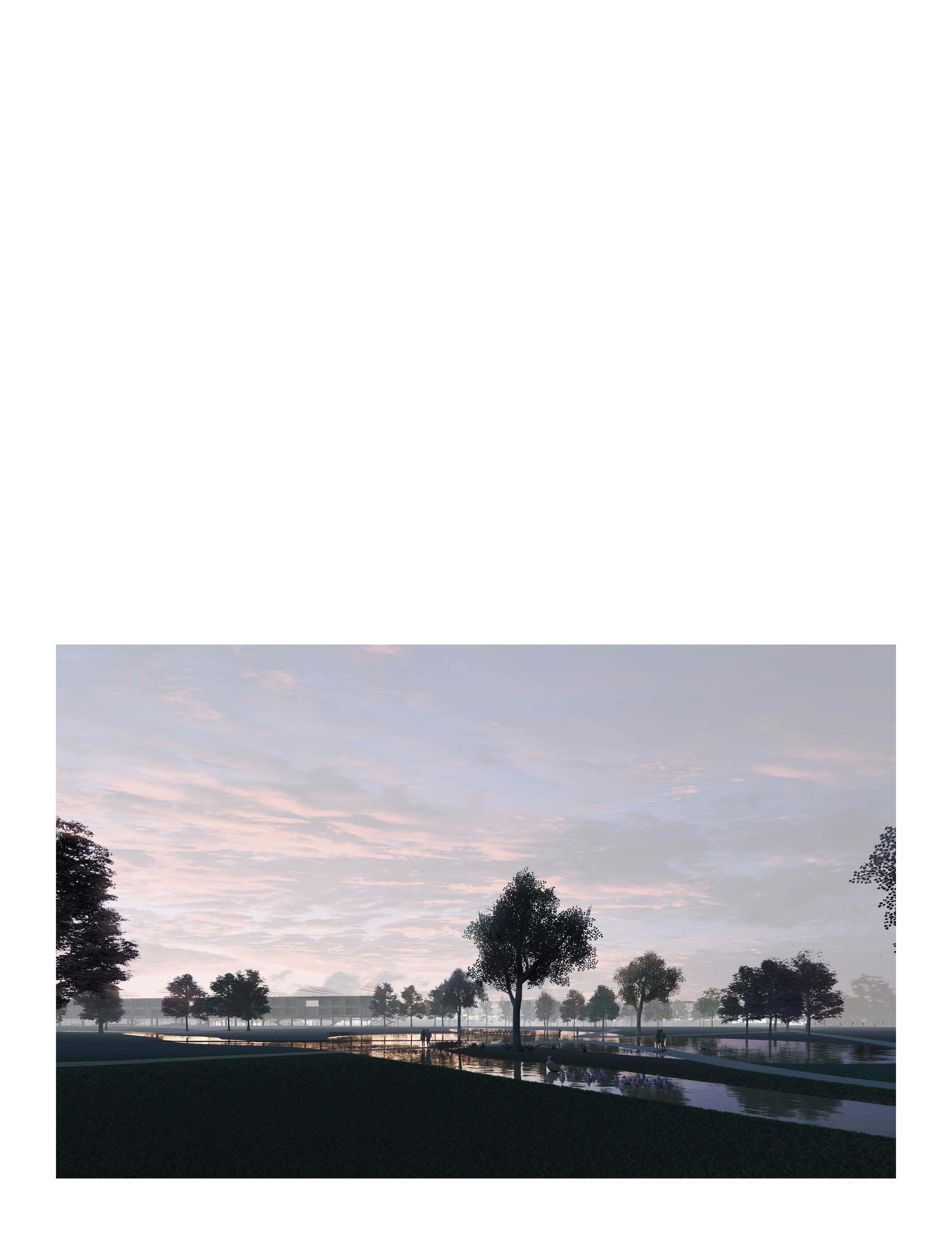
Pennington Park A New Lifestyle of Senior Living A1

2020 Spring

Professor: Bruce G. Sharky

Individual Design

Graduate Studio Design Award for Design Excellence

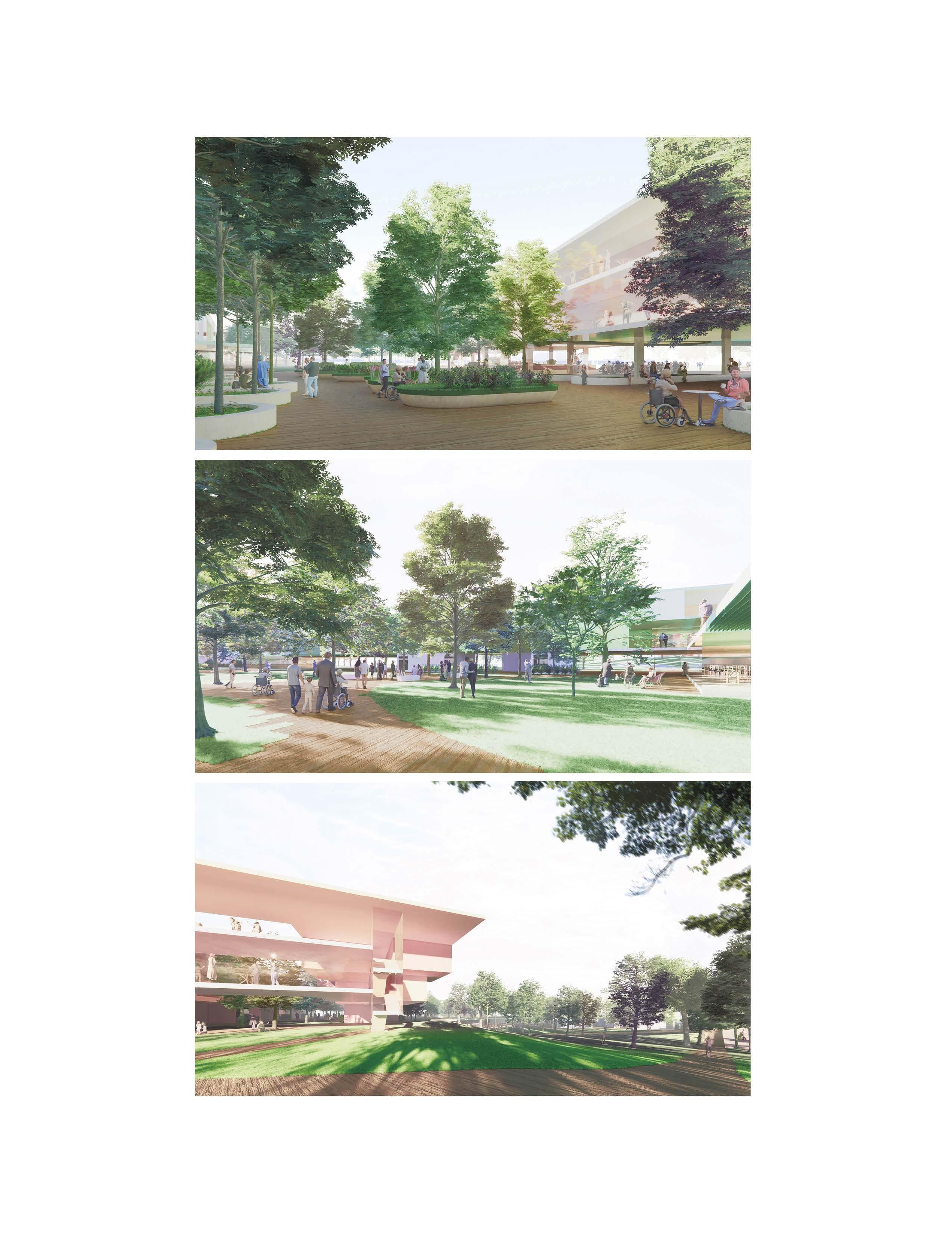
Care for senior residents should include healthcare and active living. The overall health and welfare can be achieved by both professional facility and engaging built environment. A more proactive senior living would encourage residents to interact with neighborhood, with landscape, and actively developing new lifestyle and hobbies.

Integrating both architecture and landscape space, both daily enjoyment and professional caring, the actively connected space and activities would provide a dynamic spectrum for individuals with different mobility and activity levels.

Design an Active Living Spectrum

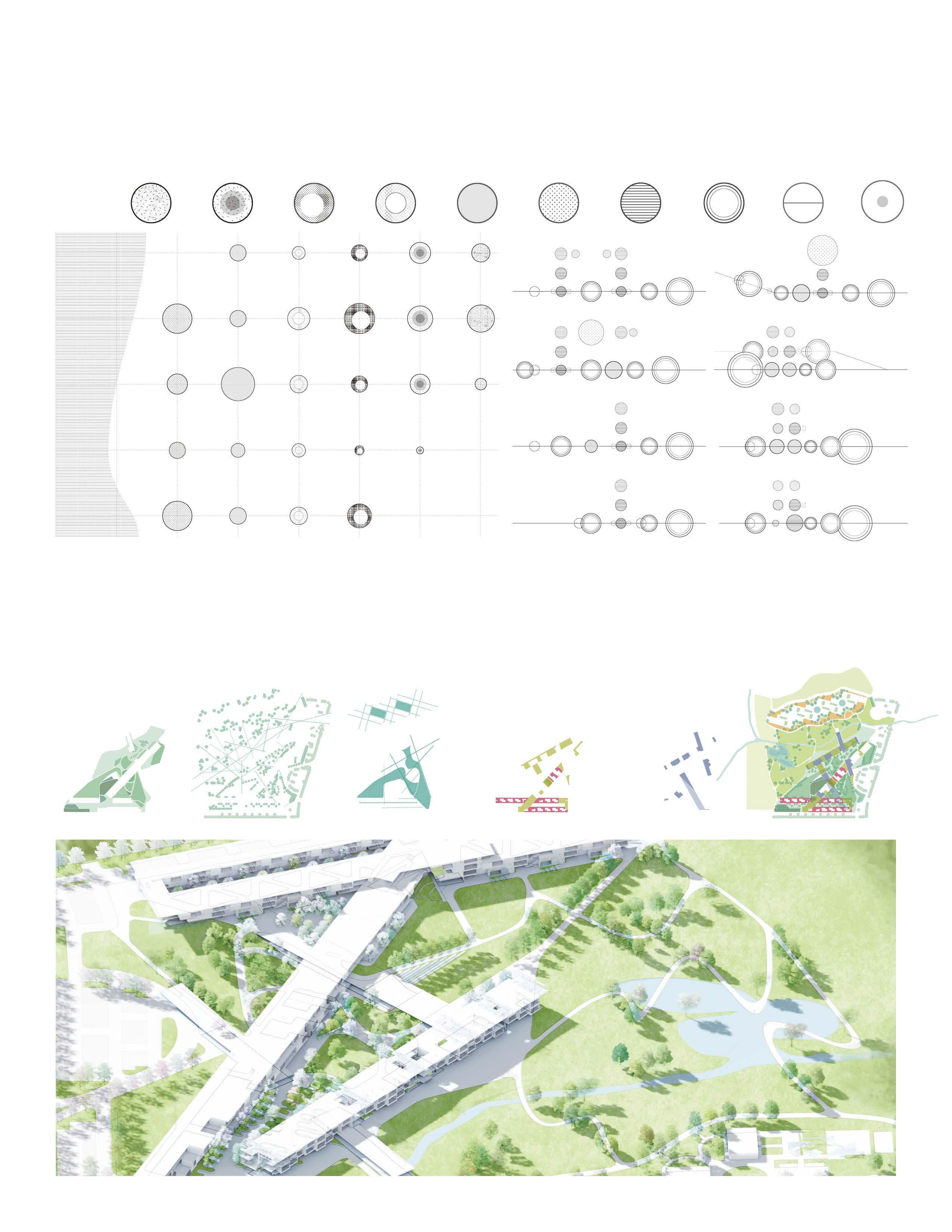
Outdoor Space

Designing

Living Space

Designing the Combination of different living units in the building would need to fit caring requirement while also promote a enjoyable and social lifestyle.

Master Plan

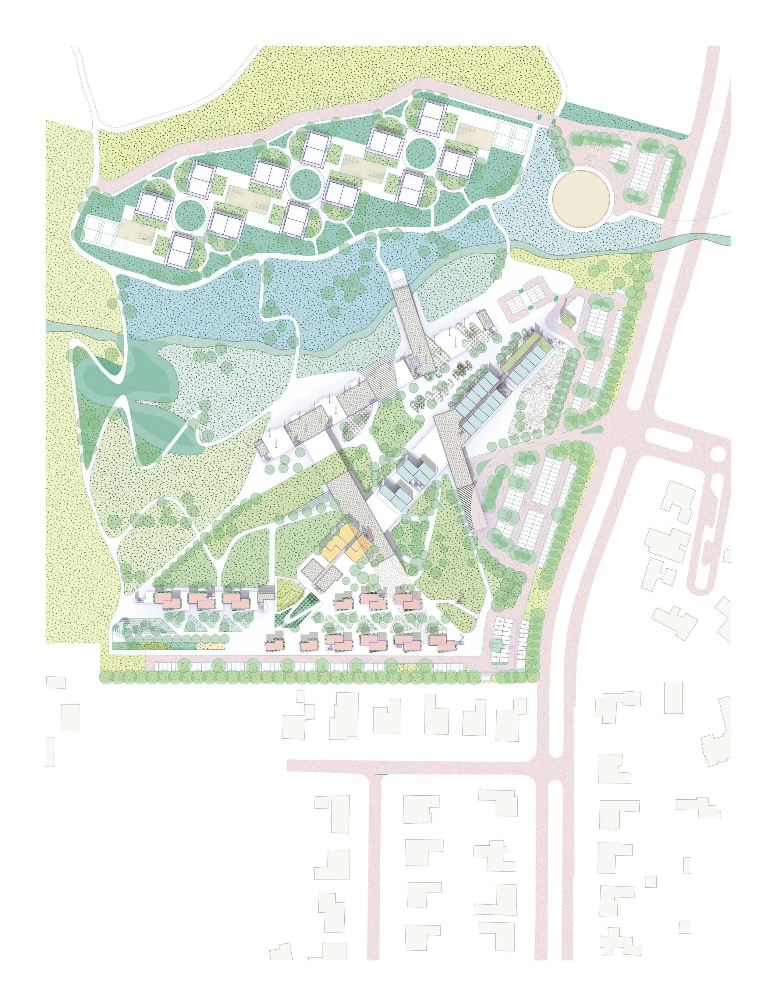
The Courtyard

Canopy Plaza

Veggie Garden

Sitting Stage

The Forest

The Tunnel Assisted Living

Healing Garden

Central Lawn and Plaza

Grass Slope

The Meadow

The Lake

The Park Bridge

Independent Housing Tennis Court

The Restaurant Parking for customer

Existing Pennington Trial Alternative Trail

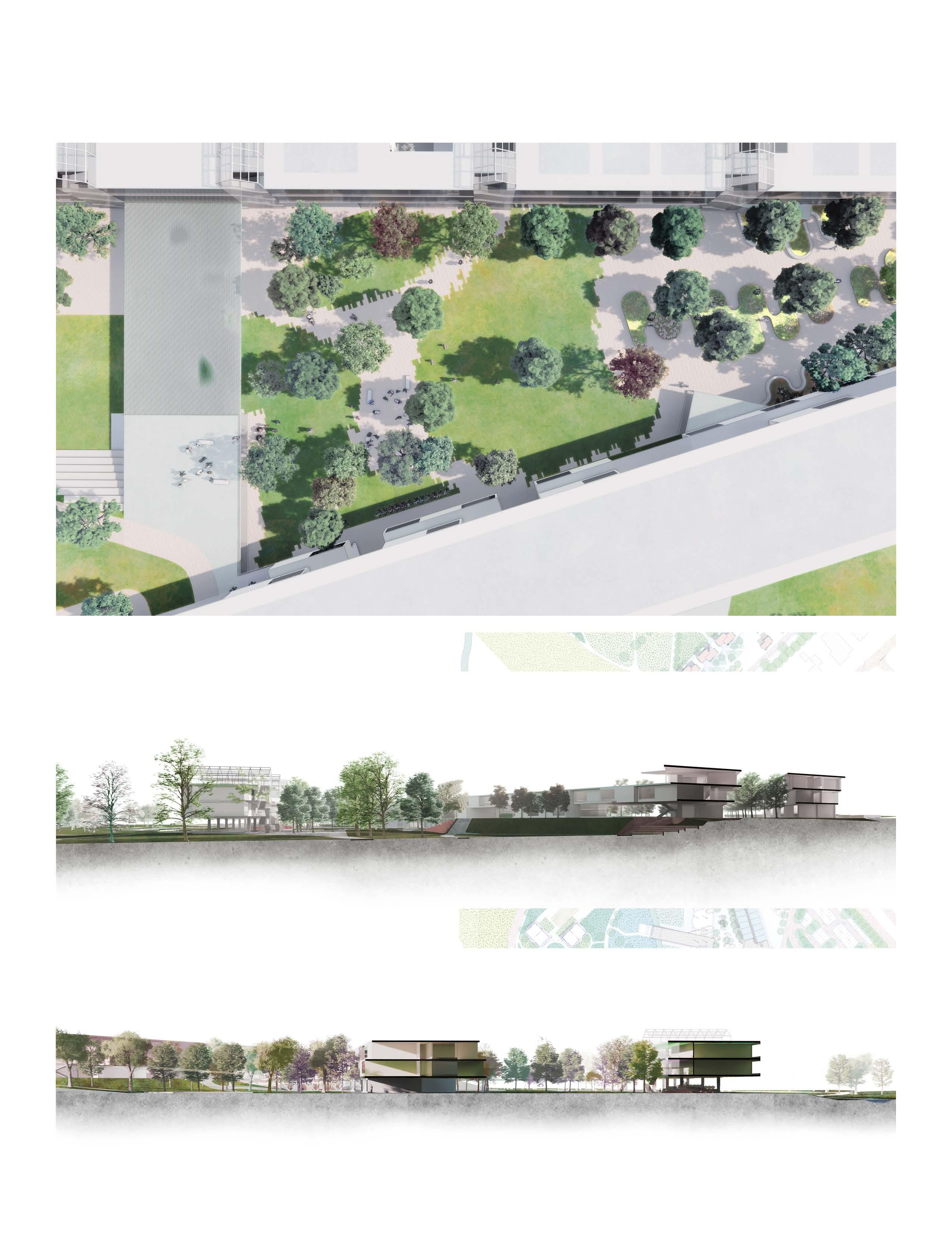
Housing Units & Combination

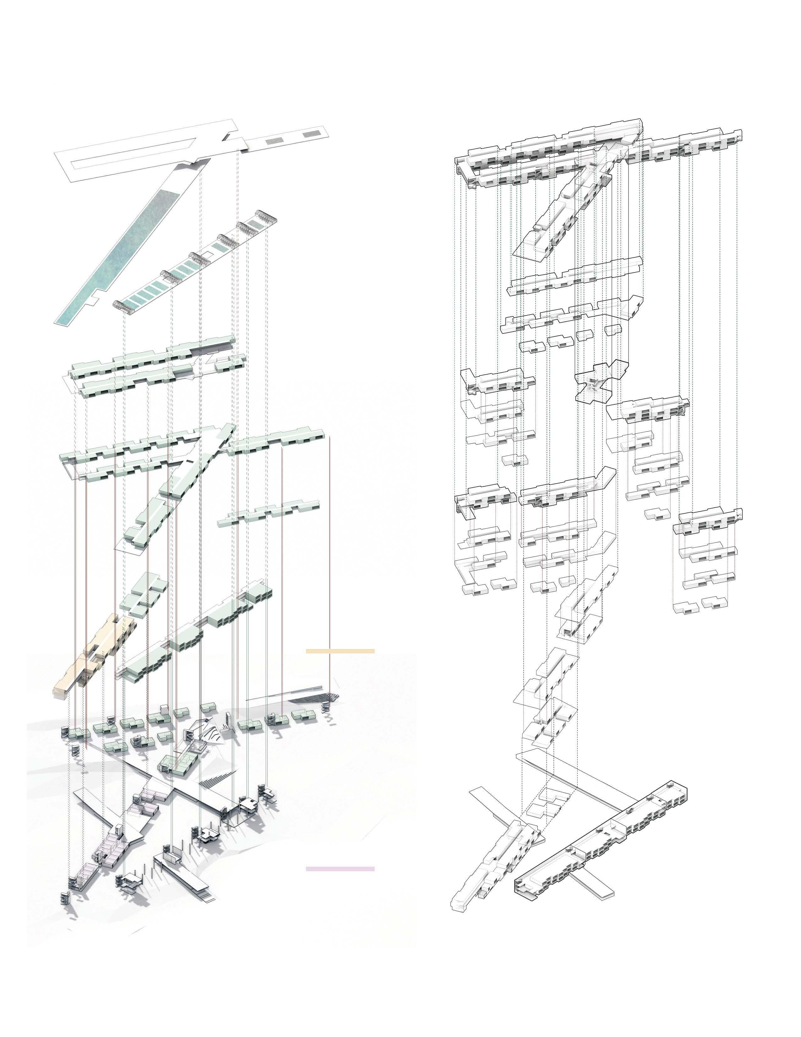
In a time of emergency like pandemic, independent living apartment s are regrouped into 13 units, each featuring accessible stair lift or elevator, and collective space for social activities. Part of the central space of the apartment is also available for medical use (A). The Enjoyment, The Studio are then turned into multi-function service place.

Assisted Living

Call of River: Relink New Orleans to the Mississippi River A2

Spine

CBD and French Quarter

Popular commercial tourism street & block

Audubon Park

Existing parks

Marginalization

Inequality, and the waterfront seems to be forgotten.

2018

Professor: Lake Douglas Individual Design

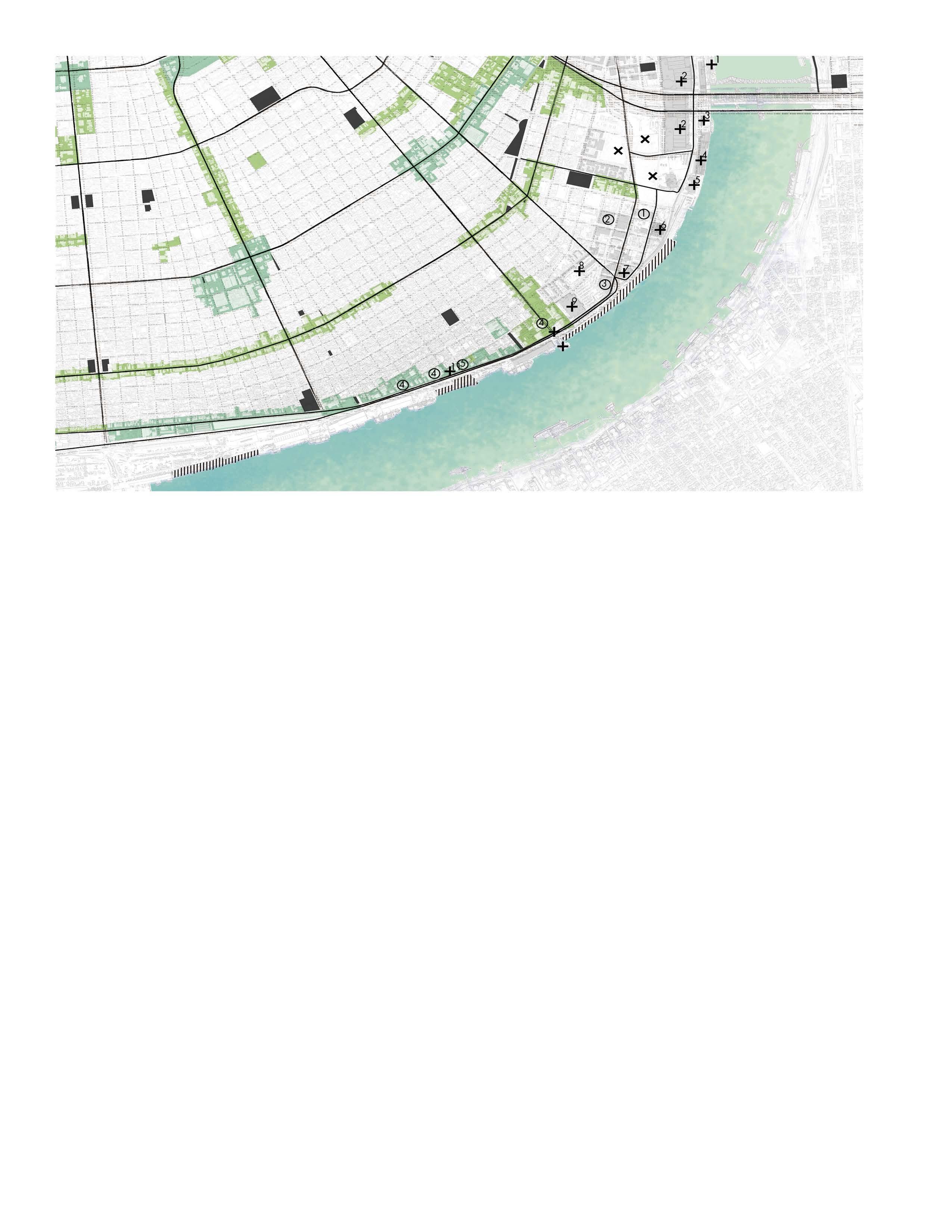
Waterfront of New Orleans, which ought to be a most active space in the city, is now marginal and forgotten.

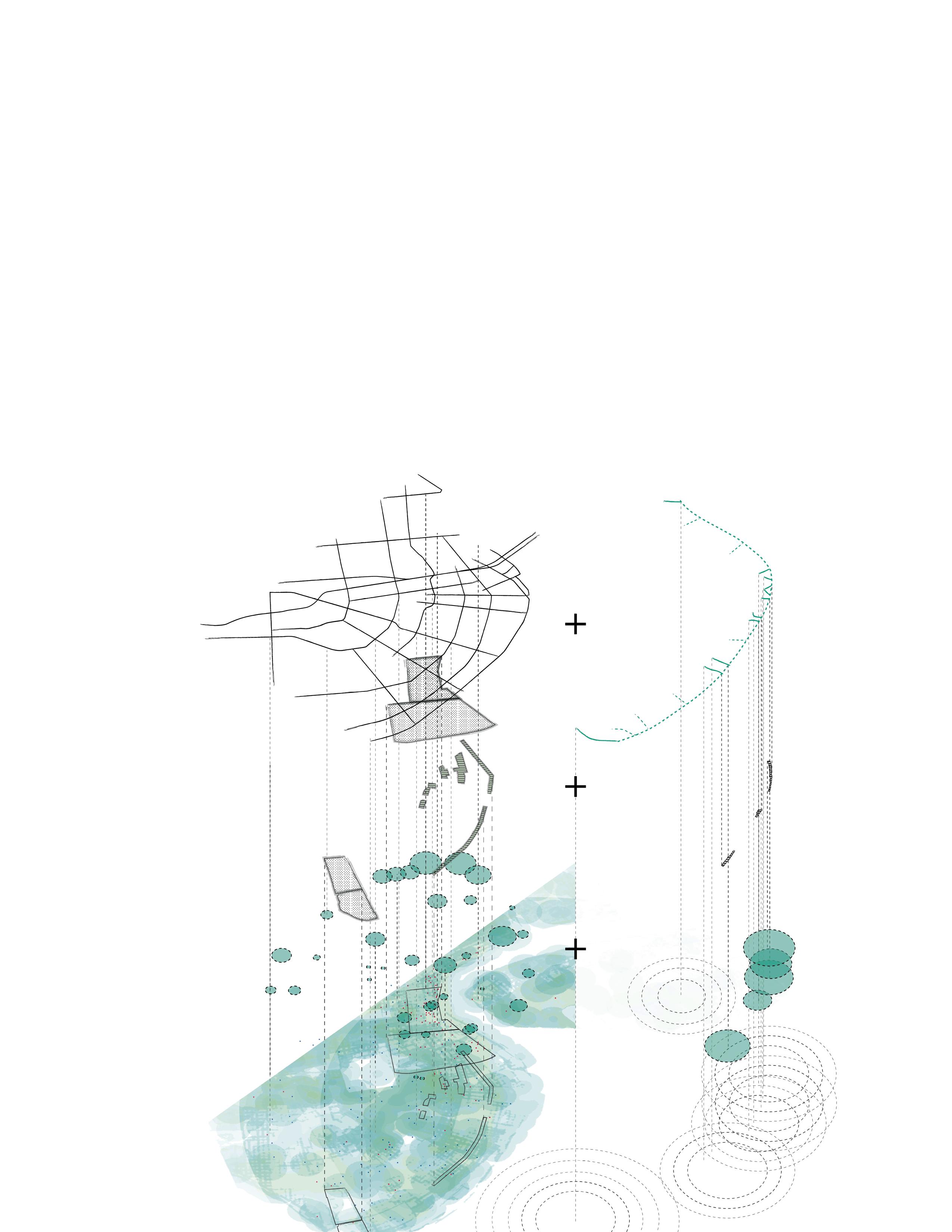
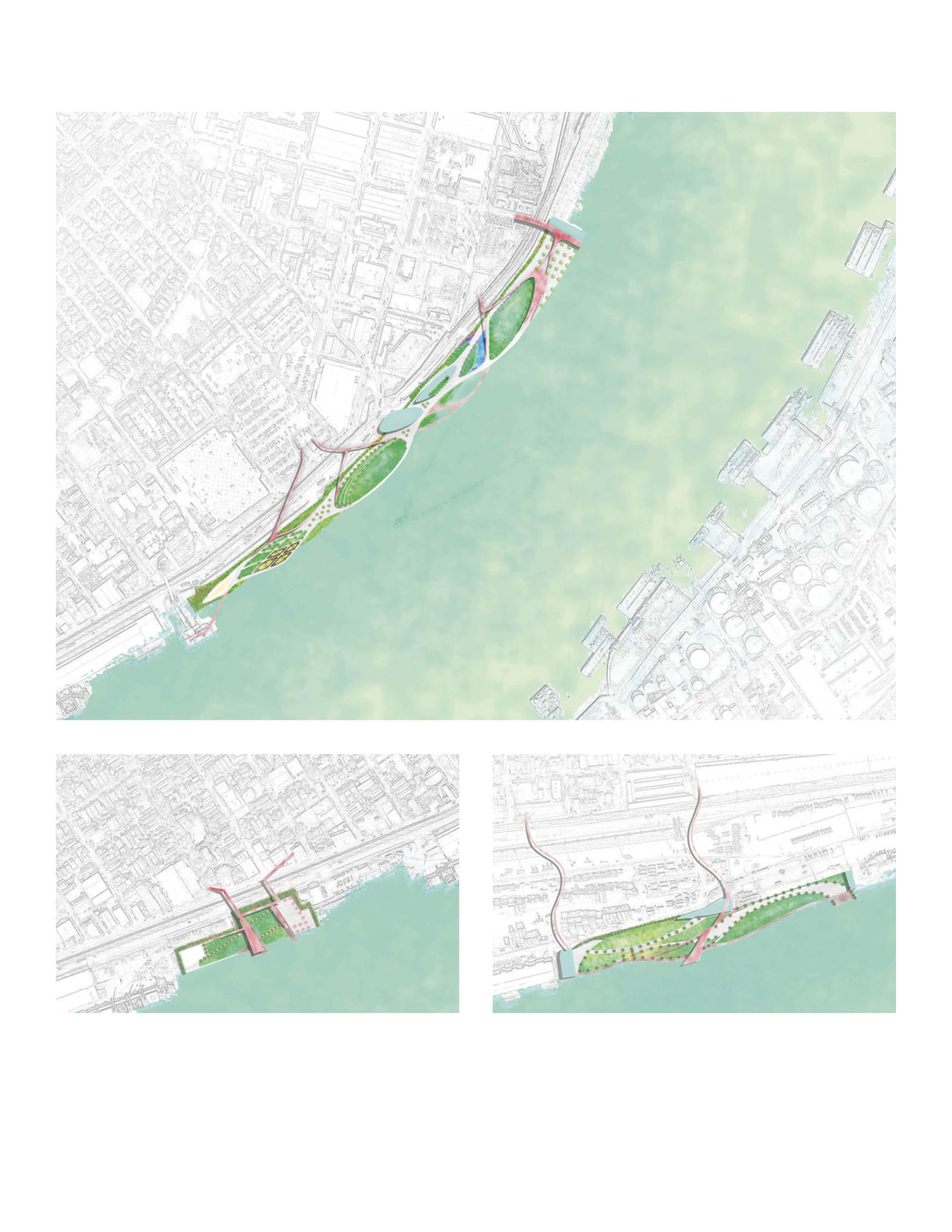
Reflecting on historic river-city relationship, deconstructing space prototype from downstream, parsing interrelationship between upstream stakeholders, and recombining all these elements and mapping on context, this project tries to transformed waterfront space into an open and active belt, connecting people, city and Mississippi River, linking Audubon Park with downtown waterfront.

Seeking Next Parks!

Grown spine

A smooth walk along waterfront from Woldenberg to Audubon

Frontier

A new way to experience NOLA & embrace life.

Radiation BOOM!

A smooth & walkable belt all along waterfront from Woldenberg to Audubon Park

Potential spot

1.Cruise terminal

center

River & Coastal Center

Gras world (Kern studio) 5.River City Venue

6.Power plant (developer purchased) 7.Apartment 8.Shopfront 9.Walmart

10.Gretna-Jackson Avenue ferry

11.Camp Bow Wow

Vacant lot

Unrelated 1.Used car dealer

traffic division

repair

supplier

Mixed-use medium density

Mixed-use low density

Parks

Context of Selected Sites

A

EXPO facility, riverfront open space & facility, supermarket, brewery power plantation, warehouse, vacant lot equipment store, auto repair, NOPD

Active Unused Others

vacant lot

Further distance

Current user & potential user

Potential place for development or connection (offsite)

Manifesto

Potential

Downtown, French Quarter, hotels, riverfront open space & facility, cruise terminal, Convention center, Mardi Gras World, event venue, St. Charles Ave.

CBD office workers, local residents, toursit, visitors from current waterfront

Connection EXPO facility, riverfront open space & facility, supermarket Development powerplant, warehouse, vacant lot

A outlook for downtown to riverscape, connect existing waterfront space, activate its forgotten surrounding.

Downtown

Magazine St. Jackson Ave. Louisiana Ave. St. Charles Ave.

Local residents visitors from Magazine St. pet owners.

Connection Magazine St., neighborhood business Development warehouse, vacant lot

A expansion of neighborhood, a venue for activity.

Neighborhood connection Community replenish Support

Active Unused Others

Lyons recreation center, bar & eat, retail,gym, house supply, music venue warehouse, vacant facility equipment, auto repair, storage

Magazine St. Artistic workshop Louisiana Ave. Napoleon Ave. St. Charles Ave.

Local resididents tourists. visitors from Magazine St.

Connection Magazine St., Lyons recreation center, warehouse, music & cultural venue Development warehouse, vacant facility

A epitaxy for inner vitality, making use of 3 main street encircling.

Scenery & community connection Urban &

Ship tour

Attraction

Deconstruction

From upstream - Interrelationship

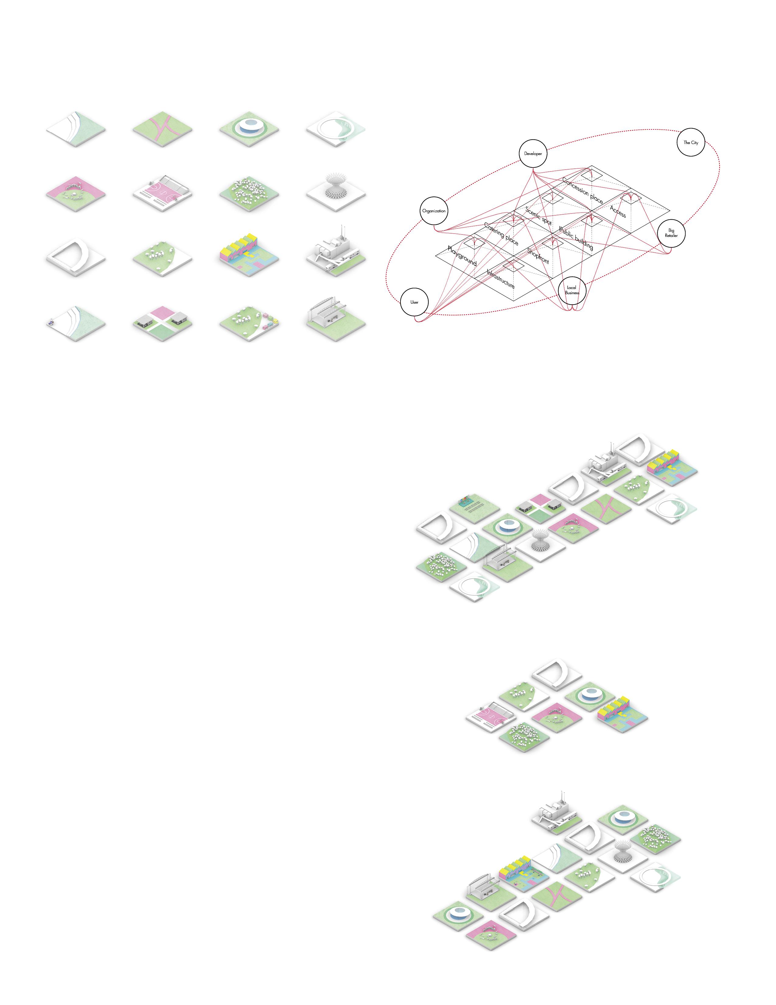
Recombination

A_Downtown

Connection

Entertainment Function Events

B_Neighborhood

Connection

Entertainment Replenish

C_Urban+scenery

Tourism

Connection Events Function Activity

Entertainment

From downstream - Request

Park Plans

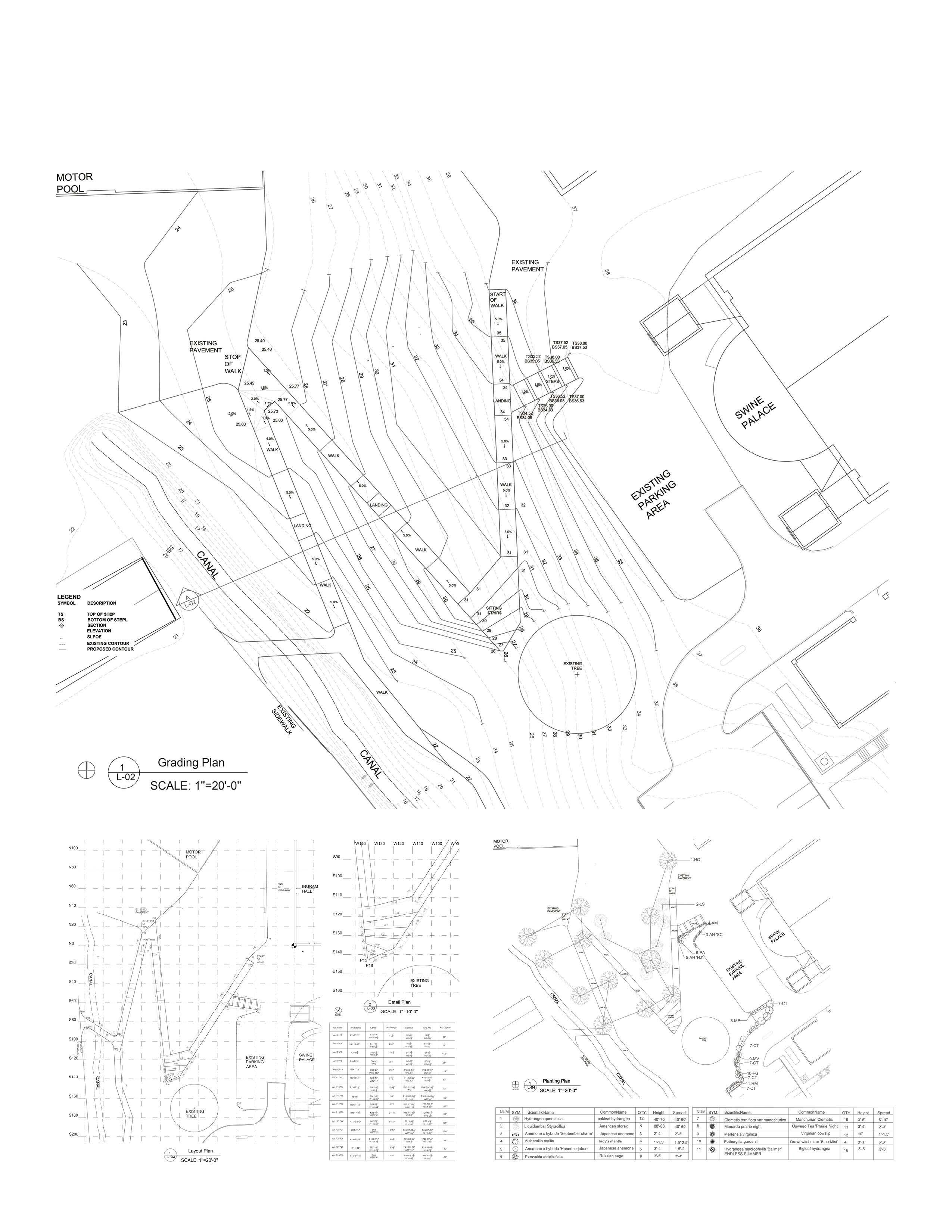
DESIGN TECHNOLOGY

Grading & Documentation A3

Remote Sensing

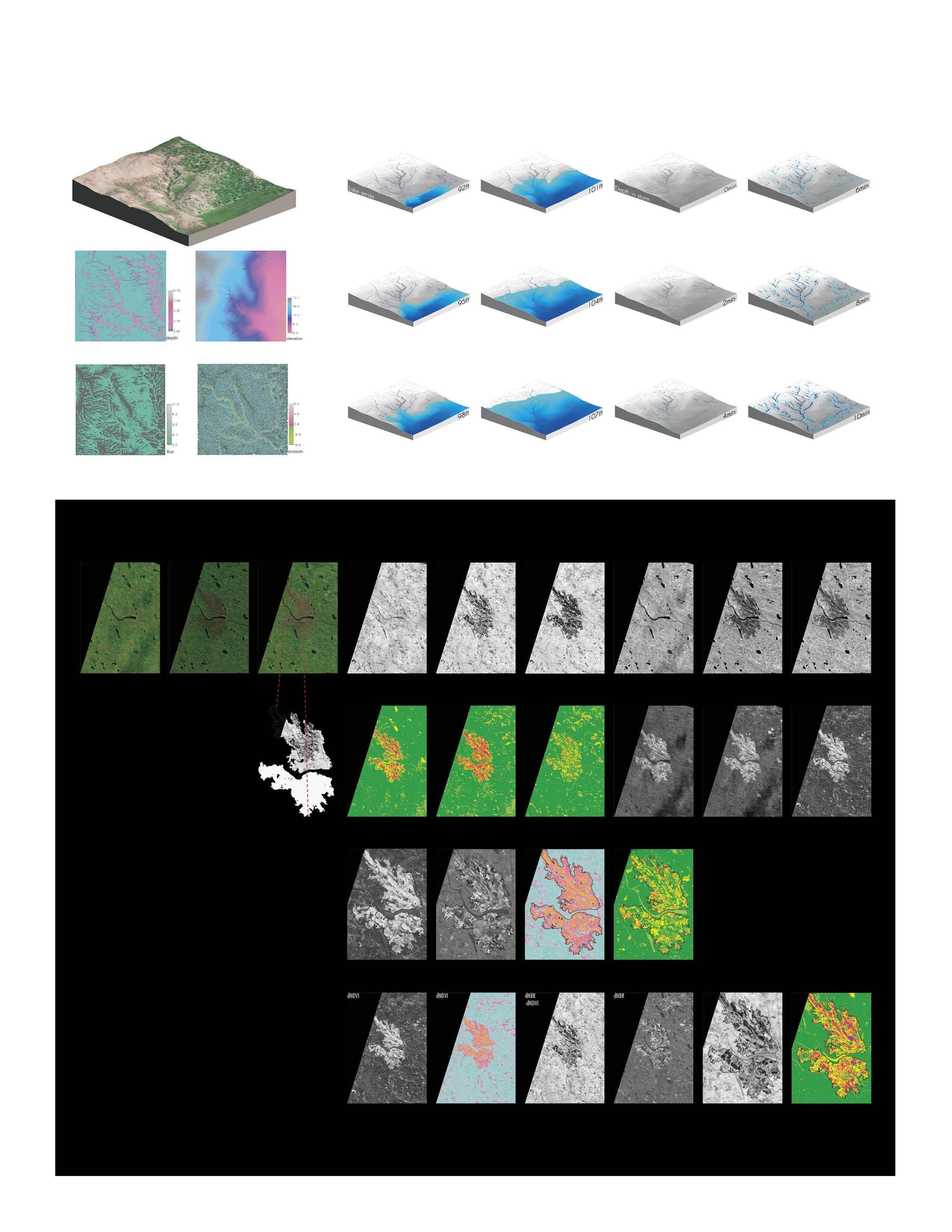
Data for lake series &

depth in storm by Joshua Black

Remote Sensing in Landscape

NBR dNBR

dNBR=

-Data dispersion (histgram)

-NBR can distinguish better and show more sensivity. Especially between the moderate‐extreme classes

-NBR and dNBR are more suitable for detecting different severity levels.

-0.500 to -0.251 Enhanced Regrowth, High -0.250 to -0.101 Enhanced Regrowth, Low -0.100 to +0.99 Unburned +0.100 to +0.269 Low Severity +0.270 to +0.439 Moderate-low Severity +0.440 to +0.659 Moderate-high Severity +0.660 to +0.1300 High Severity 20180916-20190802 20180916-20190802 Pseduo color 20180626-20180916 20180916-20190802 20180916-20190802 20180916-20190802 20180916-20190802 20180626 20180626 20180916 20180916 20190802 20190802 20180626 20180916 20190802 20180626 -20180916 20180916 -20190802 20180626 -20190802 20180626 -20180916 20180916 -20190802 20180626 -20190802 dNDVI dNDVI dNBR dNBR

Media: ERDAS Imagine, QGIS with SCP plugin and DOS1 atmospheric correction. https://issuu.com/zyq3/docs/yongqin_zhao_project

CONSTRUCTION DOCUMENTATION

B1

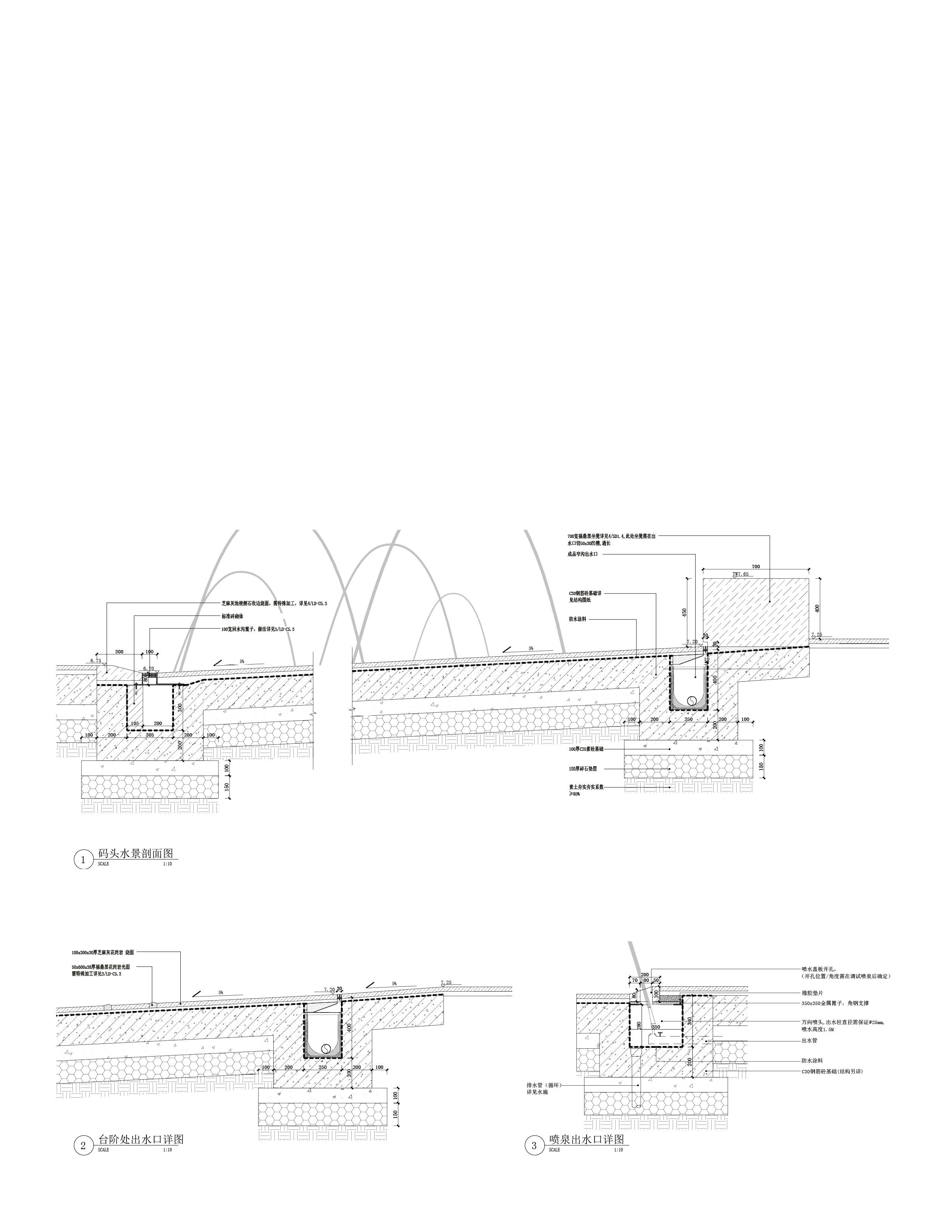
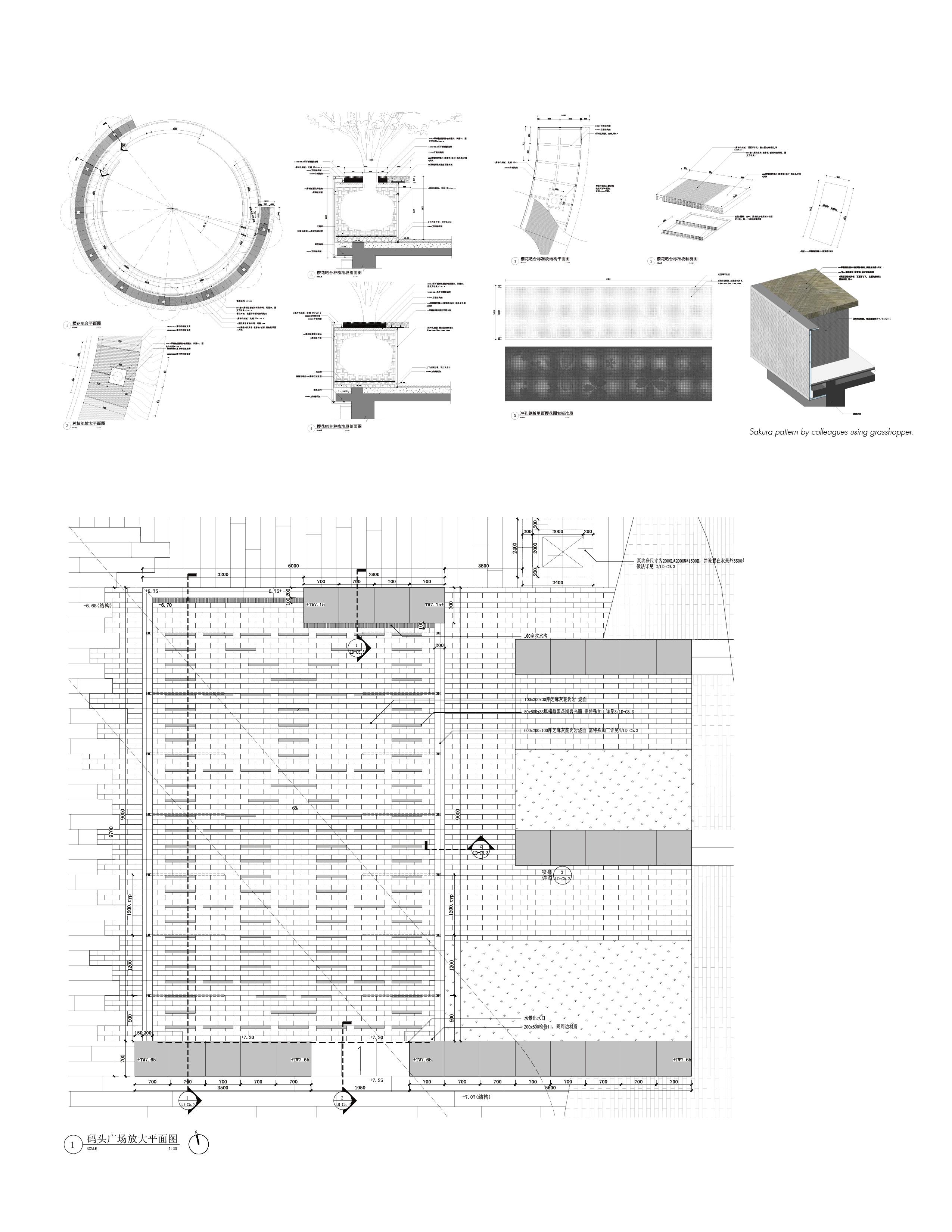
Construction Documentation

Landscape Details

Professional Work at Z+T

2019

Professional Work at Z+T Landscape Architect

Water Feature with patterned bricks

Design: Yongqin Zhao, Siyuan Lou

Dawing: Yongqin Zhao, Siyuan Lou

Supervisor: Hua Zhao

Details of outdoor furnishing

Drawing: Yongqin Zhao

Supervisor: Hua Zhao

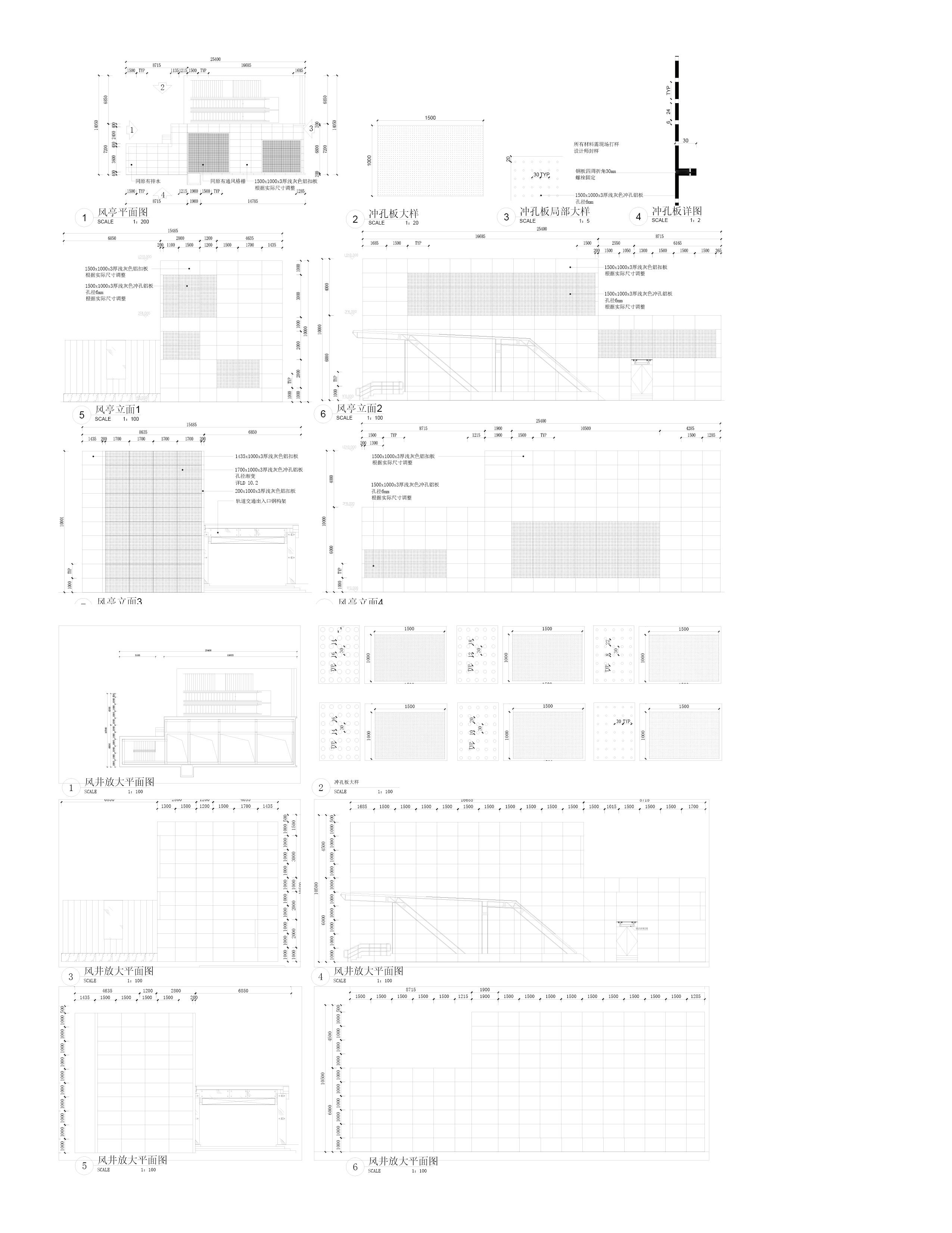
Facade Design

Professional Work at Z+T

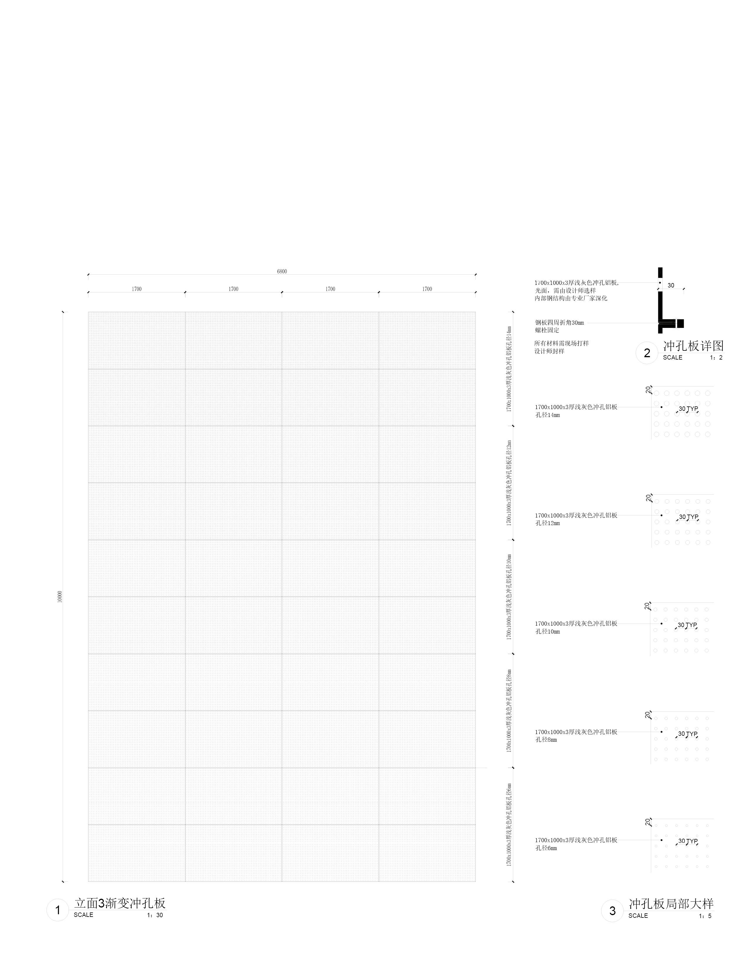
Perforated Plate of Ventilation Facility for Subway Design: Yongqin Zhao, Cheng Xie Supervisor: Min Xu

PROFESSIONAL DESIGN WORK & TECHNOLOGY

B2

Professional Design Work & Technology

2019 - 2022

Professional Work at Tianhua Urban Design Lab & Dreiseitl Concept, Schematic Design, Design Development, Competition, Design Guideline, Site Design and Master Planning

Landscape Urbanism

TOD Landscape

Professional Work at Tianhua

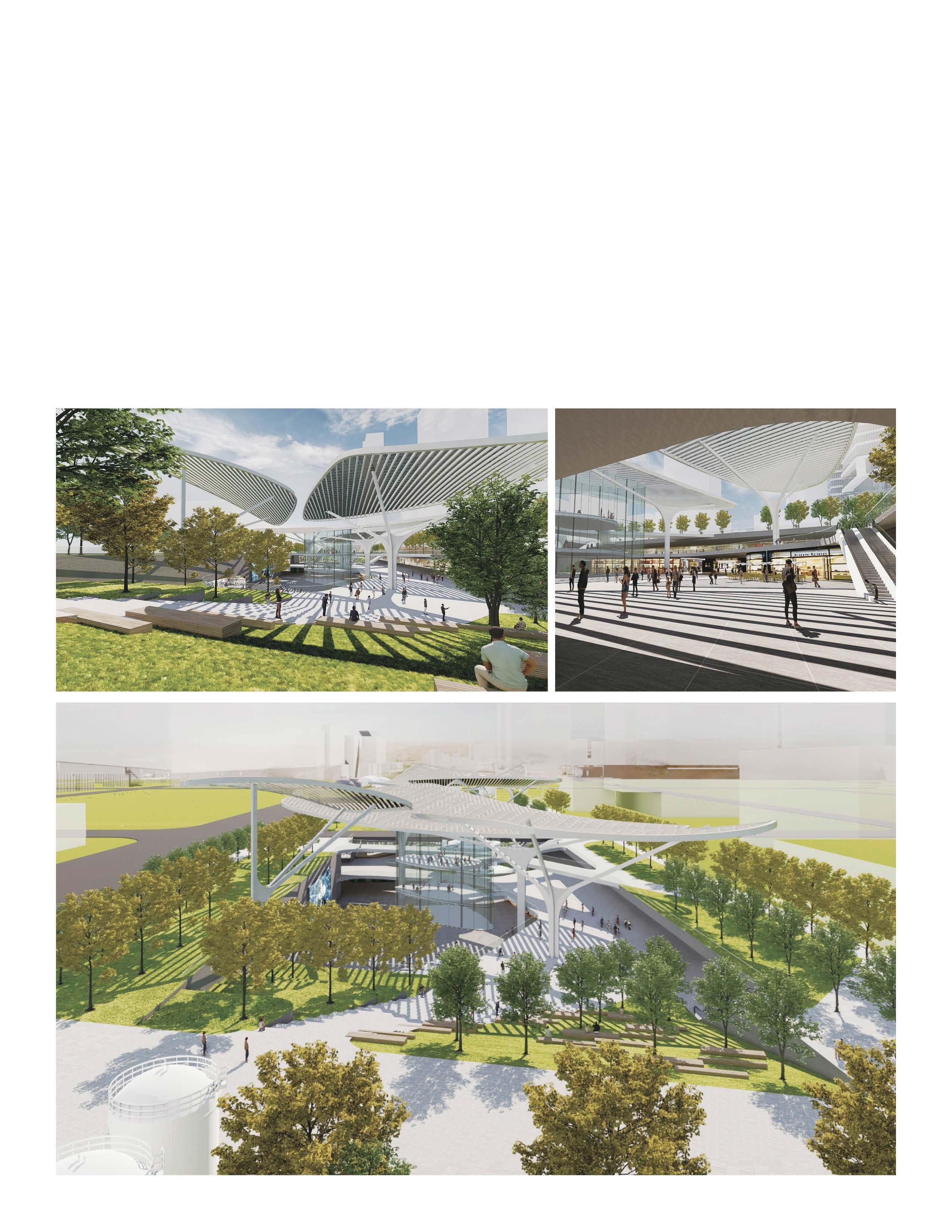
Could a subway station become a park?

This design tries to make full use of subway connectivity(up to 3 lines join together) and surrounding context (office underground) to open up the station. Circulation, accessibility, cultural facility, and retails are weaved in this design, where people gather, stay, or commute.

Visualization of elevated park

Design: Yongqin Zhao

Render: Yongqin Zhao

Supervisor: Jie Bao

From terrace at ground level

From subway station entrance/exit at B2 level

Birdeye view from park

Residential Urbanism

Professional Work at Tianhua

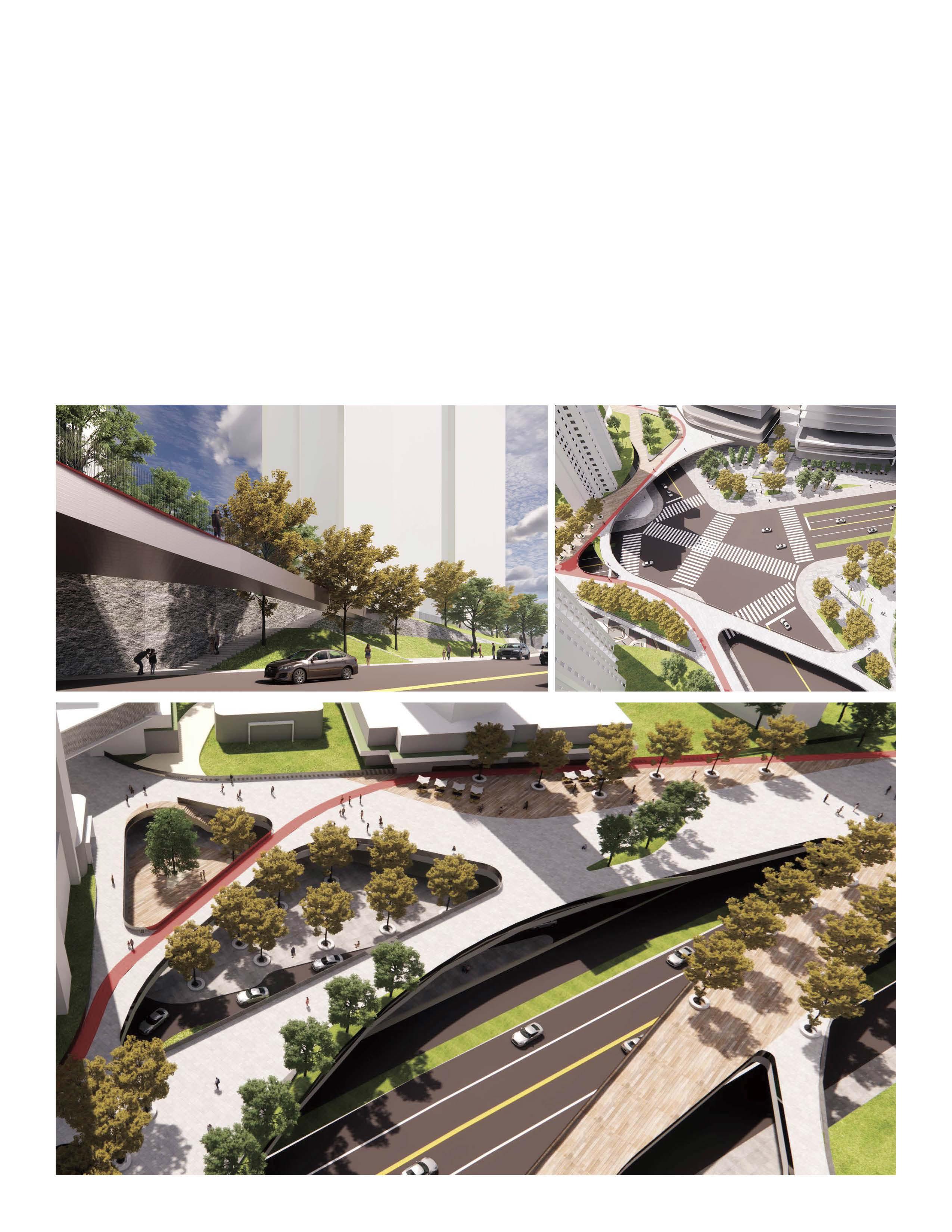
Landscape helps envision super community. Imagine a area floating above urban street network, and residents celebrating their life wherever they prefer.

To achieve this, vehicle and service circulation are placed on the ground floor, so that all active activities would take place on the elevated floor. Elevated parks connects communities, municipal sidewalk, and public service together.

Visualization of elevated park

Design: Yongqin Zhao

Render: Yongqin Zhao

Supervisor: Jie Bao

Connection to Ground Floor Sidewalk

Great intersection

Community Entrance, ground + park level

B2:Professional Design 2

Landscape Urbanism

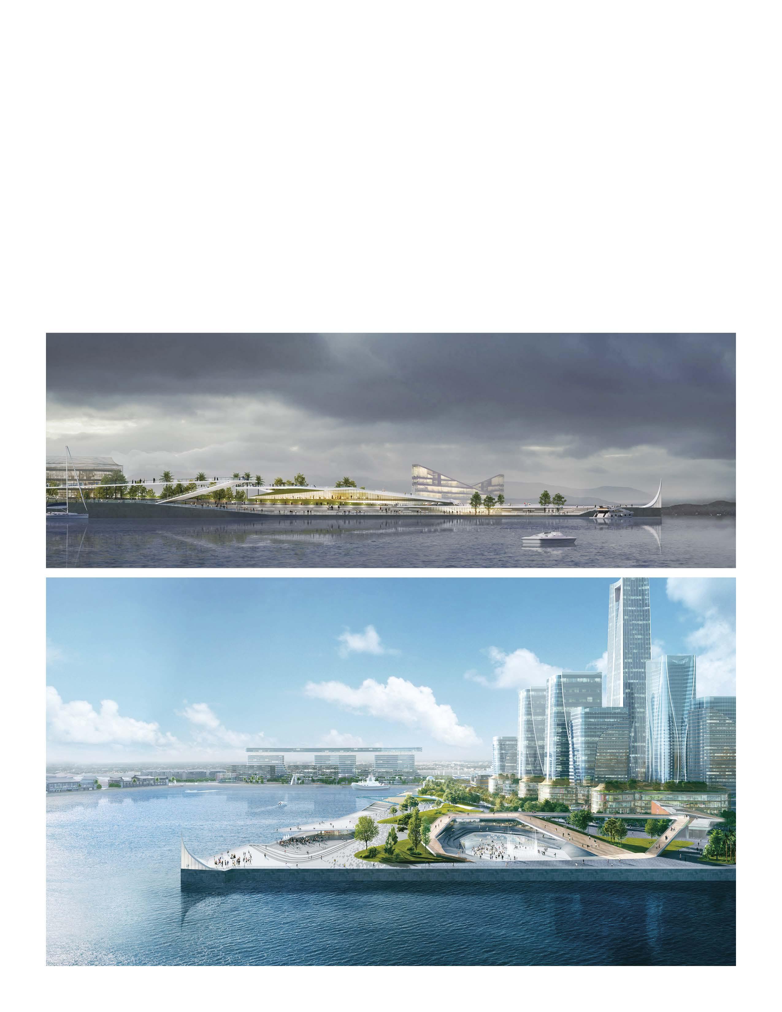
Waterfront Park Center

Located right near the CBD and newly proposed Convention center, this would host vistors with all purposes, as well as daily activity of the locals.

This park design features green area and terrains, a water-facing amphitheatre, cafe and dining area, and pedestrain brdge system that connect all above together with urban context.

Visualization of the community center

Design: Yongqin Zhao

Render: Ginsun Rendering

Supervisor: Jie Bao

Professional Work at Tianhua

Parametric Design

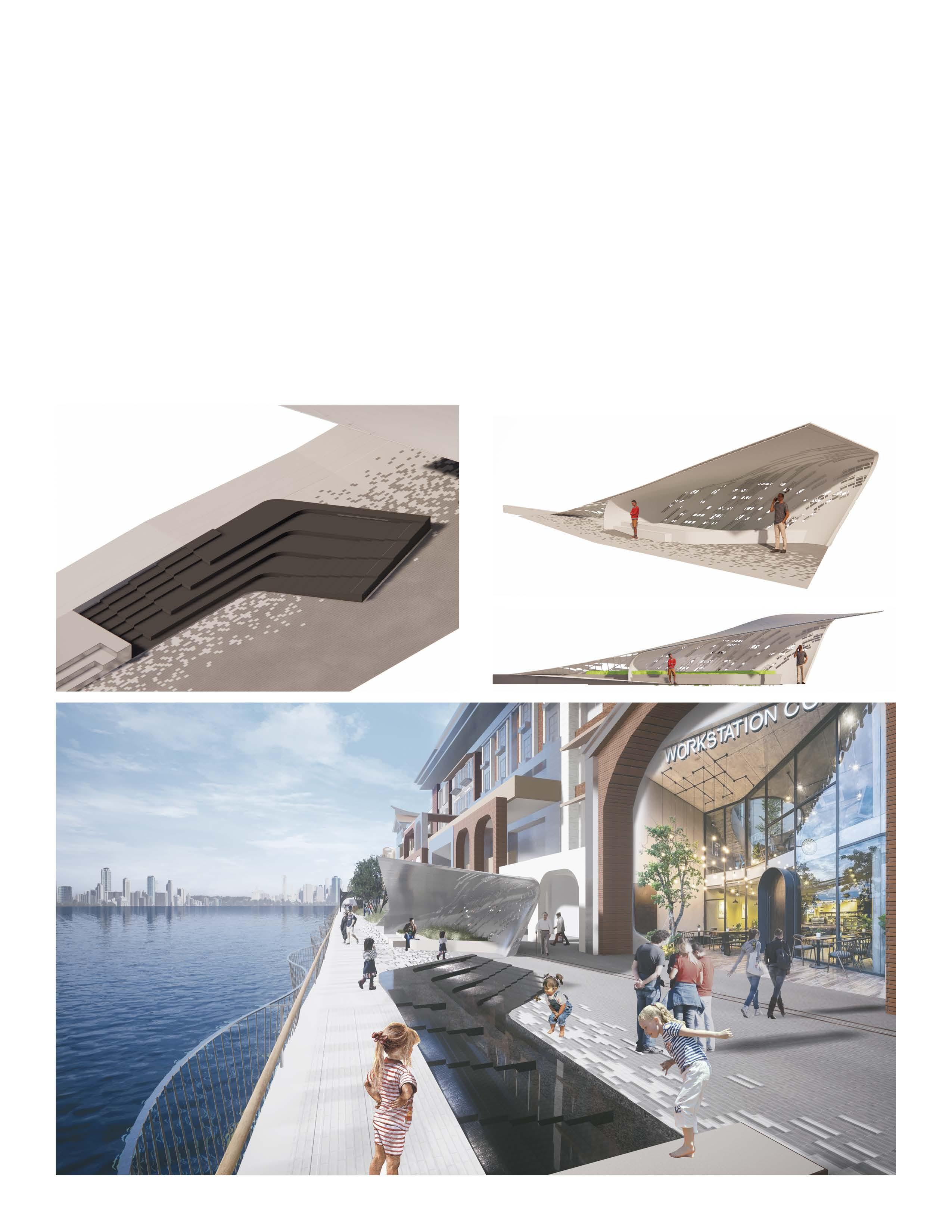
Reflection Pool

This design integrated ADA standard grading detail and pavement, retails, and water collection features.

Grasshopper is used in the design.

Details and Visualization

Design: Yongqin Zhao

Render: Yongqin Zhao

Supervisor: Jie Bao, Jiayan Bao

Professional Work at Tianhua

Parametric Design

Pavilion

Professional Work at Tianhua

Design: Yongqin Zhao, Jiayan Bao

Grasshopper & Detail: Yongqin Zhao

Render: Yongqin Zhao, Jiayan Bao

01.Set Magnetic field

Generate magnetic lines of induction along the surface of the pavilion.

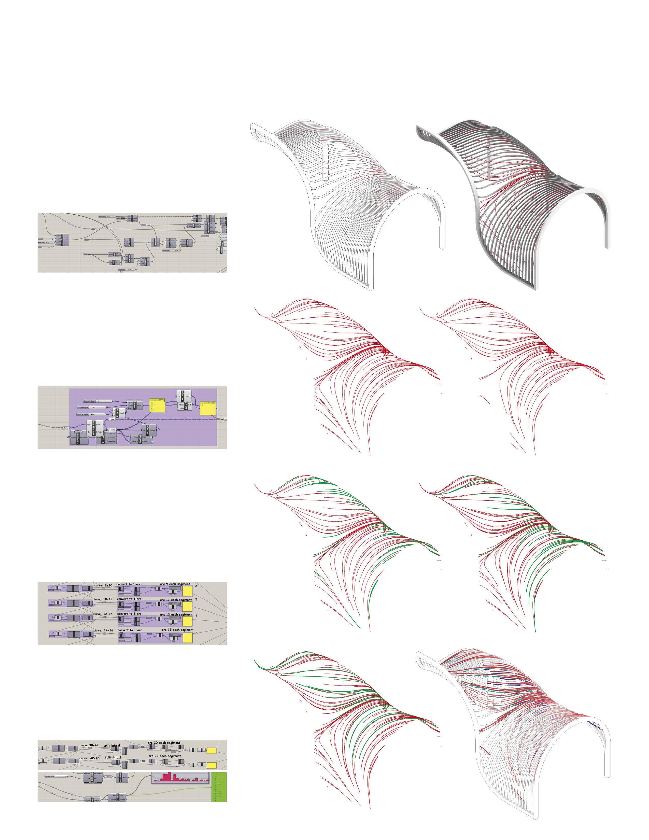
02.Filter Magnetic lines

Remove part of the magnetic field lines in the high-density area according to the frequency distribution in the x direction

03.Classify & Regularize lines

Classify lines of magnetic induction into 3 types according to their length, and convert them into 2, 4, and 6 arcs. Screen out arcs with appropriate lengths. The arcs are again grouped into intervals by length. Normalize the length of arc again in each interval.

04.Classify & Extrude

The distribution of the final arc lengths is shown below. Based on the angular proximity between the arc and the surface of the pavilion frame, 4 different sizes of section depth are set.

Pavilion & Planting design (Day)

Lighting(pavilion+pavement)

Night

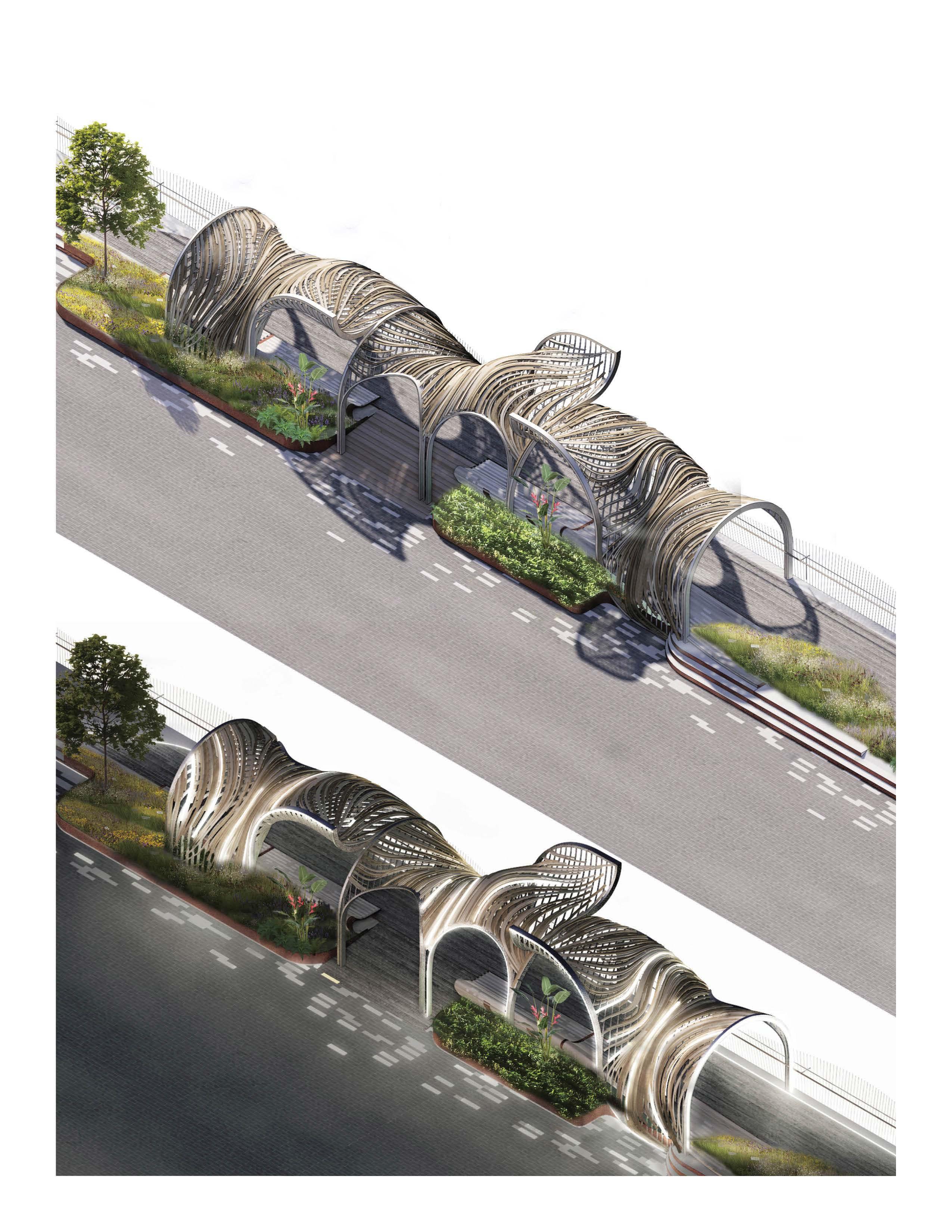
Urban Design and Streetscape

Streetscape System

Professional Work at Tianhua

Design: Yongqin Zhao

Render: Yongqin Zhao

Supervisor: Jie Bao

Pocket Park

Architecture

Community Center

Professional Work at Tianhua

Cantonese have a strong internal connection to their clan, and ancestral hall and banyan tree are the two most important triggers to this feeling.

In the development of a housing project, I designed a modern community canter just right near the ancestral hall, and connect the two with similarity in form, space, and the circulation.

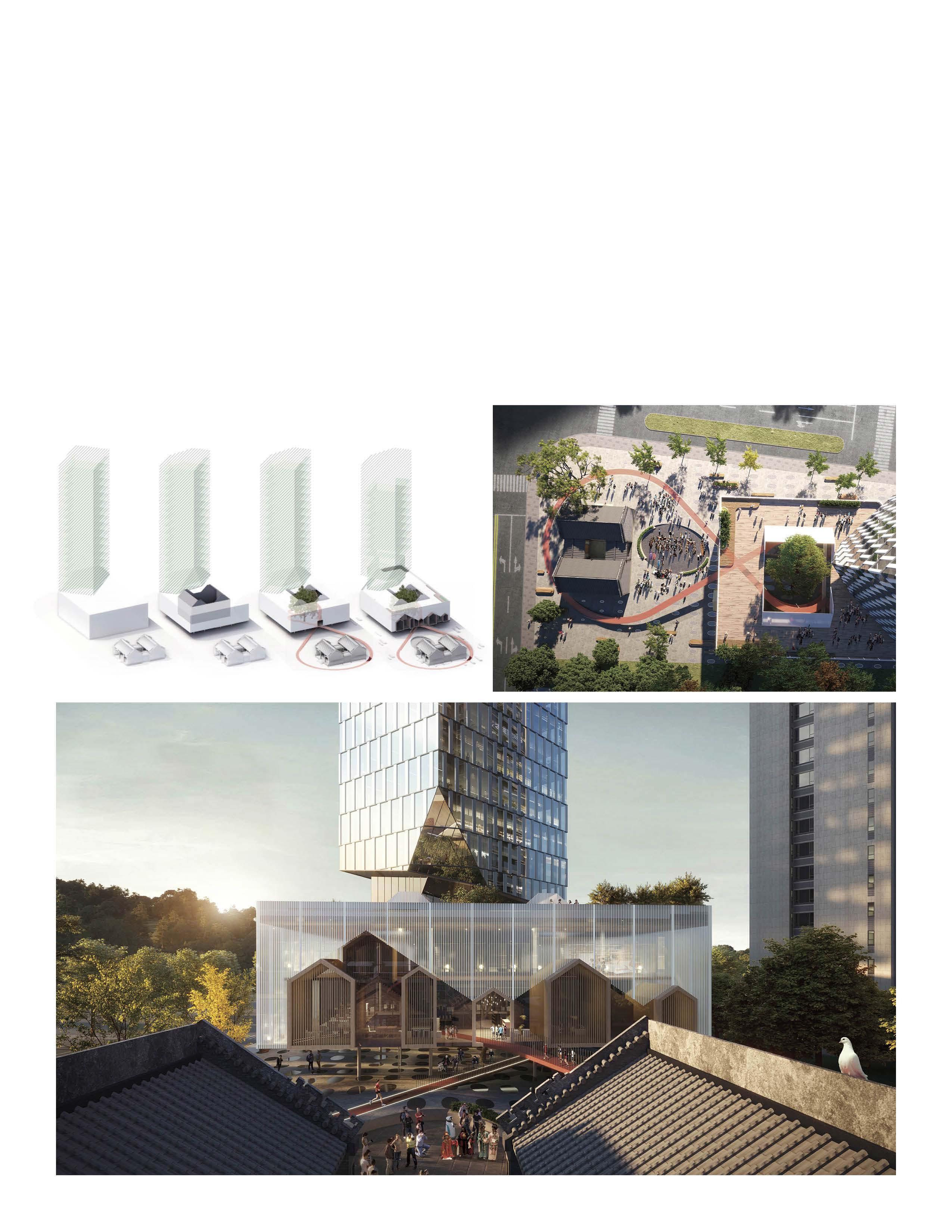
Mass generation of the community center

Design: Yongqin Zhao

Drawing: Yongqin Zhao

Supervisor: Jie Bao

Visualization of the community center

Design: Yongqin Zhao

Render: Ginsun Rendering

Rural Revitalization

Professional Work at Tianhua

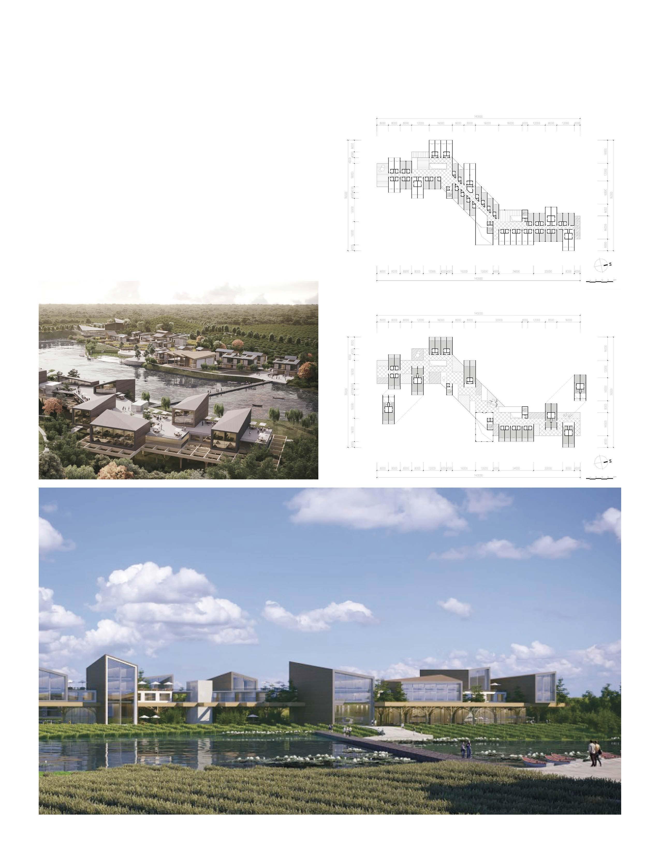
To create a scape of “home being”, for local youngsters that leave there hometown to make a living, and for visitors from cities to experience a memorable lifestyle.

This hotel integrates different housing units in the farmland, vegetation, and terrain, as well as local’s handcraft studios.

1 - 2

Floor plan of the hotel (part)

Design: Yongqin Zhao

CAD Drawing: Bowen Liu

Supervisor: Jie Bao, Jian Zhen

Visualization of the hotel

Design: Yongqin Zhao

Render: Ginsun Rendering

B2:Professional Design 6

Design

Competition & Strategy

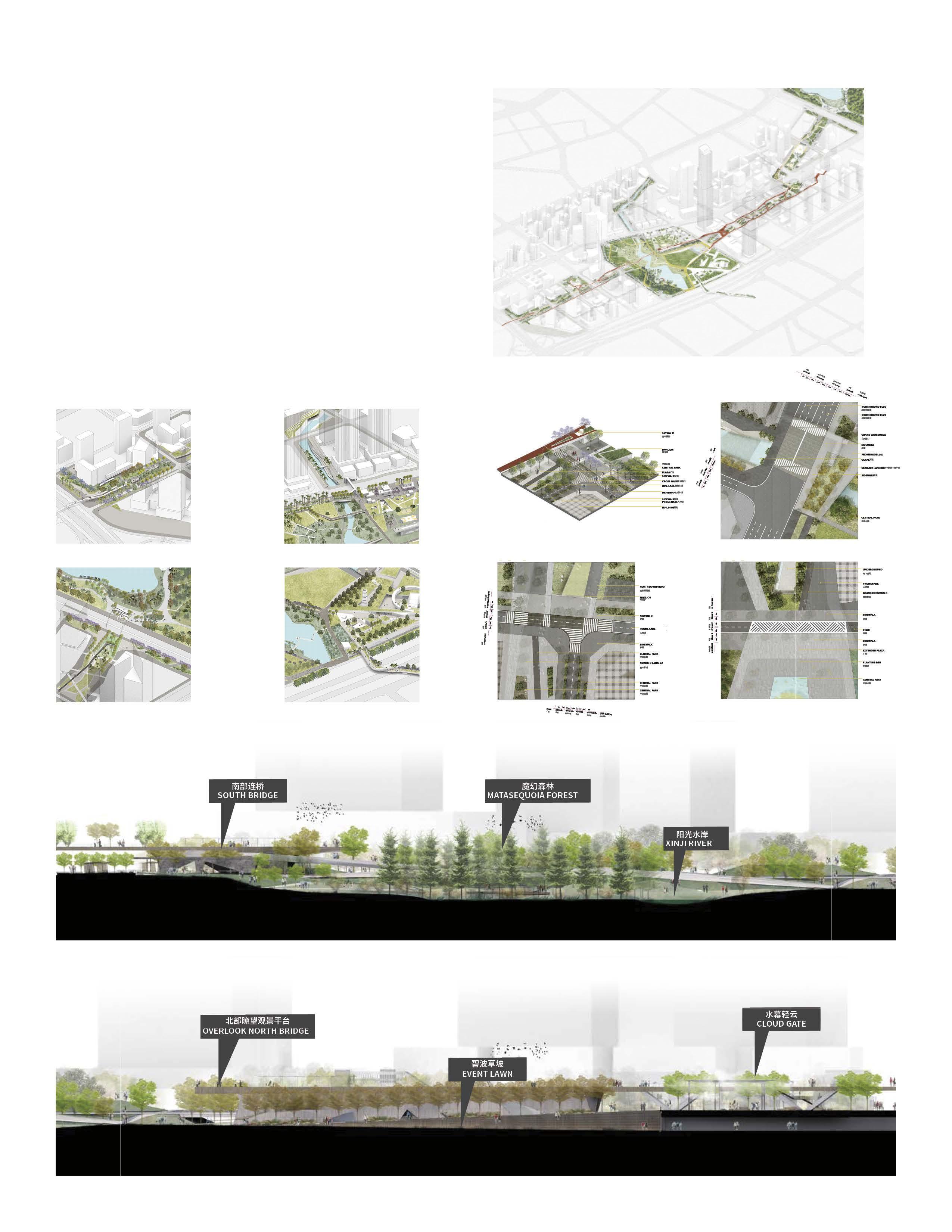
Park Interface Design

Professional Work at Dreiseitl Singapore

An integrated design of park’s interface with its urban context, including material, pavement, grading design, etc.

Park Interface

Design: Dreiseitl Team,Yongqin Zhao

Drawing: Yongqin Zhao

Section drawing

Graphic: Yongqin Zhao

Levee Strategy

Professional Work at Dreiseitl Beijing

Design for grading and terrain strategies, including retention pond, sunken plaza, terraced boardwalk, amenities, and some urban design features.

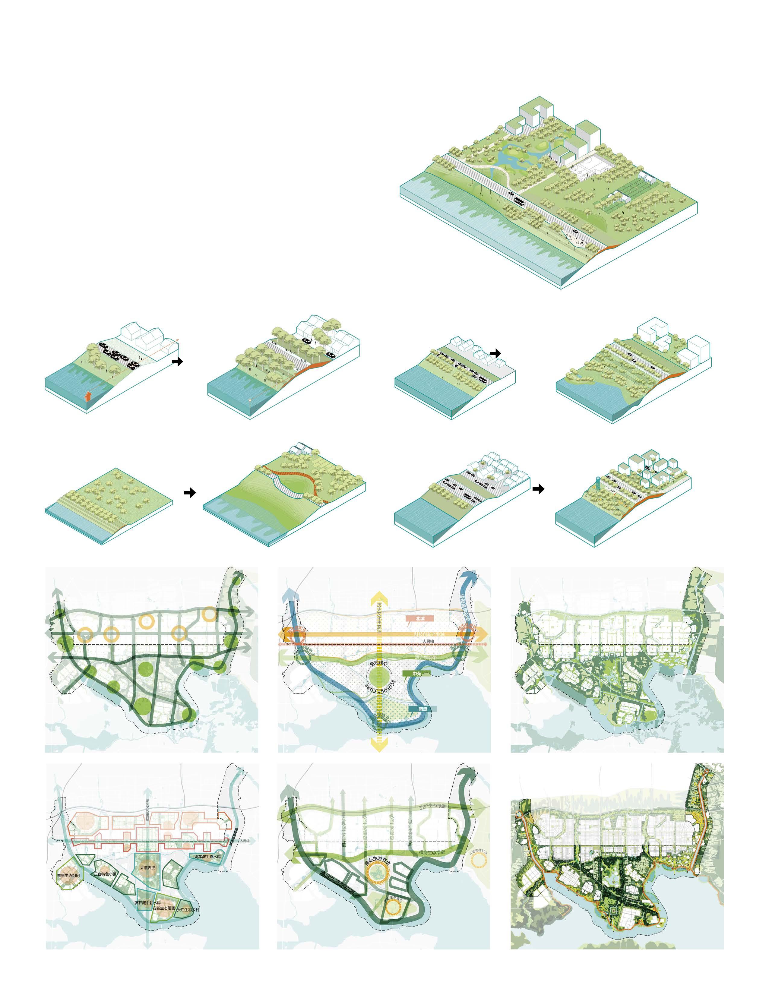
Levee Strategy

Design: Yongqin Zhao, Panpan Zhu

Graphic: Yongqin Zhao

Urban design Framework

Graphic: Yongqin Zhao

Urban elements

Spatial map

Spatial structure

C1

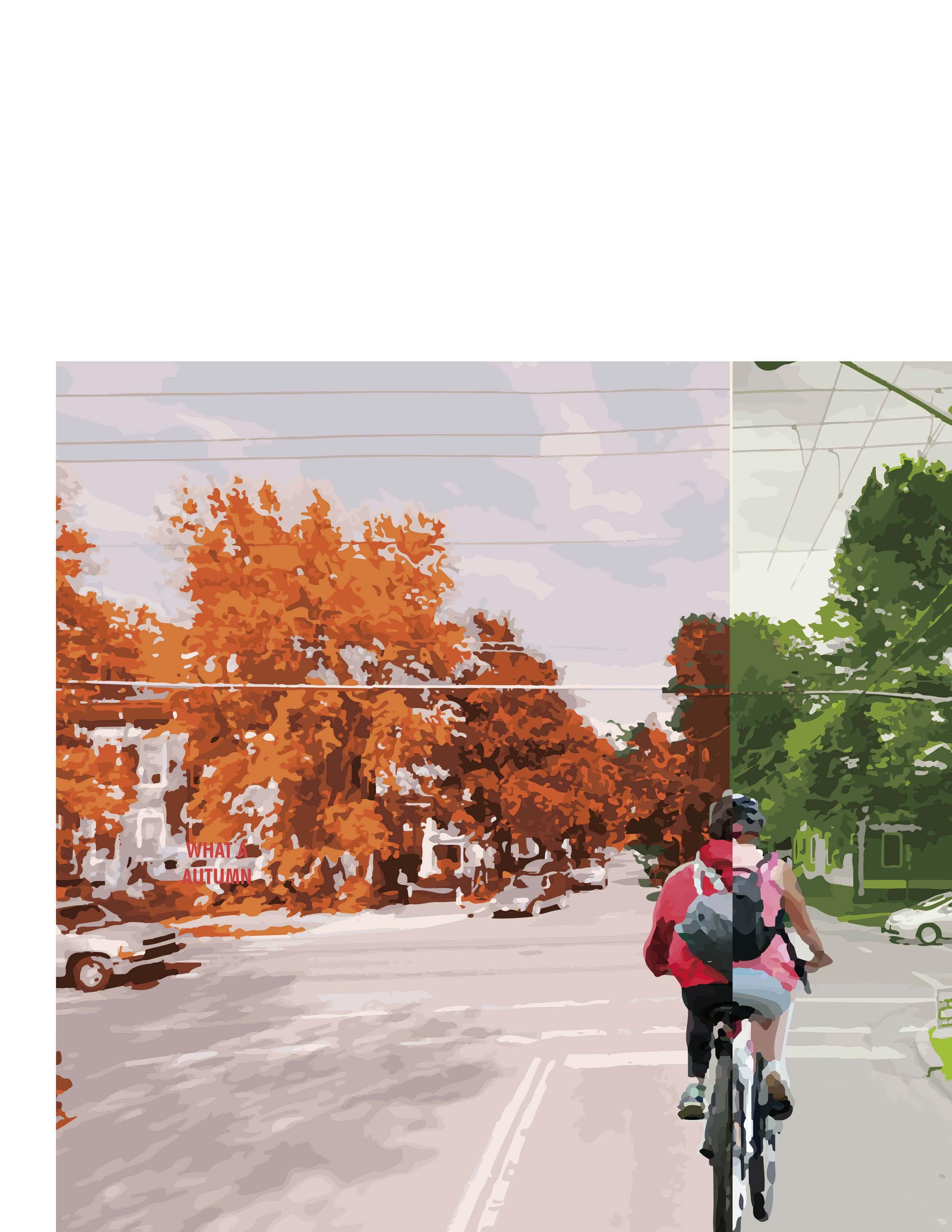
Built Enviornment and Mobility: Measuring the seasonal variations of associations between streetscape and dockless bikeshare trip volume

2023 - Ongoing

Team Leader of 5

Tool & Task

Computer Vision (MaskRCNN, Color Analysis), Model Building (OLS, SFE, SLX), Analysis & Writing, Visualization (Mapbox)

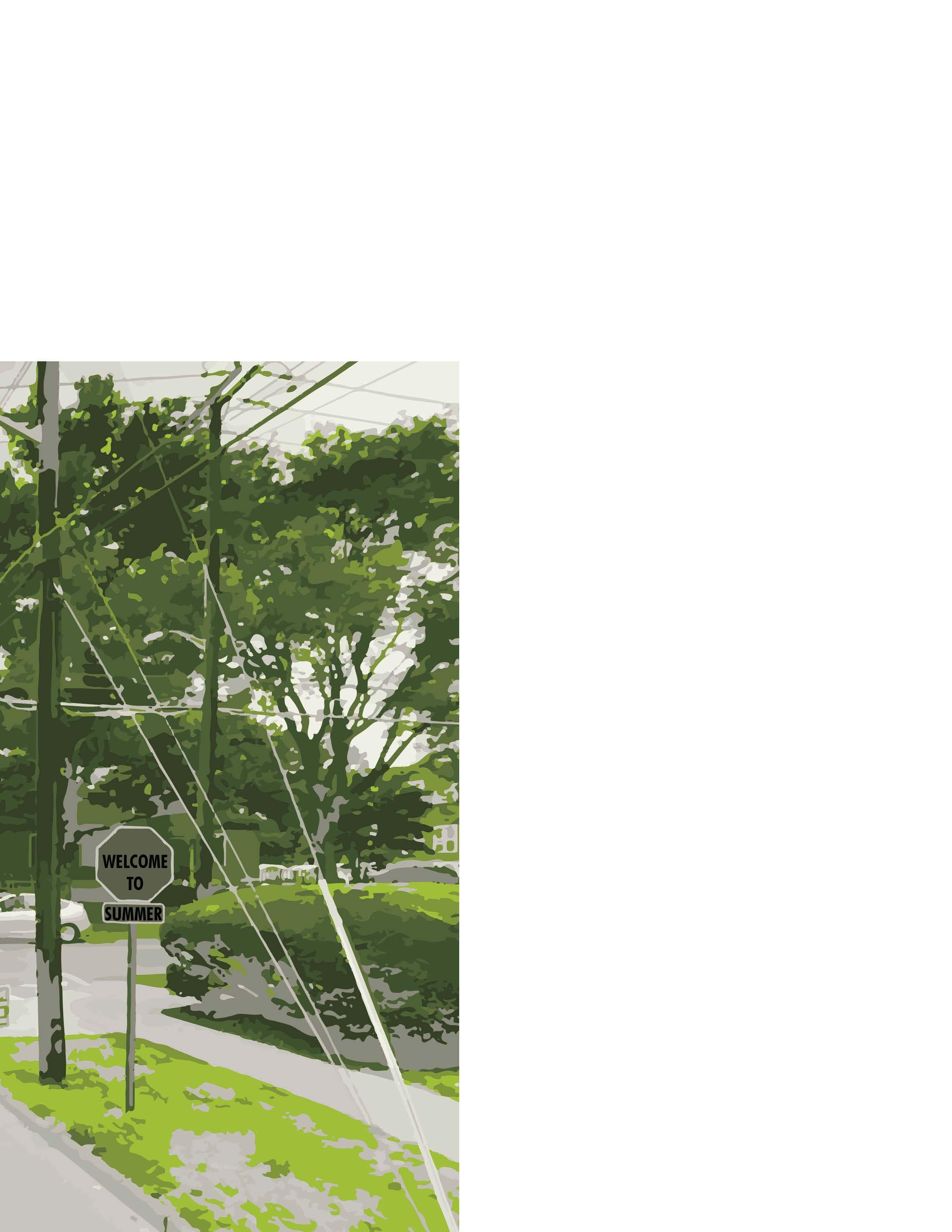
Streetscape plays a significant role in the cycling experience and the impact varies across different seasons. Most prior studies of streetscape ignored its temporal dynamic of it. And for studies of urban public mobility route choices, there has not been much focus on variables within a seasonal scale. In this paper, using a large amount of GPS bike trajectory data collected from LIME, a DBS system in Ithaca USA, we study the correlation between dockless bike sharing and streetscape, plus spatial elements in different seasons. Ordinary Least Squares Model (OLS), Spatial Fix Effect Model (SFE), and Spatial Lag Model (SLX) are built respectively. The results show that seasonal streetscape factors, such as road, car, sidewalk, grass deviation, tree lab color, and tree color deviation, have significant impacts on the DBS trip volume. But how significantly these seasonal factors influence SWR varies across summer and autumn models. Non-seasonal factors, such as land use mixed score, station, school, street network connectivity, etc., are significant for both summer and autumn models. Some non-seasonal factors only impact the DBS trip volume of one season. Seasonal subjective perception, when added in models of both seasons, helps improve the explanatory significantly. But the improvement is very slight.

The study provides a valuable reference to policymakers, urban planners, and operating companies to jointly cooperate towards a sustainable cycling-friendly city.

Related Publication:

Zhao, Yongqin , Sijia Wang, Difan Chen, Kaijie Huang, Siyuan Zhang, Waishan Qiu, and Wenjing Li. Phygital Intelligence , 211–224. Computational Design and Robotic Fabrication. Singapore: Springer Nature, 2024. https:// doi.org/10.1007/978-981-99-8405-3_18.

Background and Literature Review

1.1

DBS and street built environment

1.2

Seasonal variations and cycling behaviors

1.3

1.4

Research gap and contribution

Factors influencing cycling activities can be categorized into these domains: (1) demography. (2) the integration of bike sharing and public transportation. (3) land use and point of interest(POI). (4)built environment. Built environment factors have shown significant explanatory power in understanding travel choices (Cervero, 2002). Eye-level greenness has a positive association with cycling occurrence(Lu et al., 2019), and aquatic areas have a similar effect (Krenn et al., 2014). However, few studies specifically focus on DBS behaviors.

Seasonality in climate, affecting the natural environment and human comfort, would have an impact on outdoor activities and behavior (Ahas et al., 2007; Guan et al., 2021; Hadwen et al., 2011). However, there is a dearth of studies focusing on how seasonal change in the urban built environment, influences cycling behavior.

Focus on landscape elements that are sensitive to seasonality and essential for the cycling experience is valuable but not receiving too much attention. Which specific built environment factors have a temporal impact on bike sharing usage? Is this impact positive or negative in a particular season, and how huge is this impact? What is the difference in this impact in different seasons? These are the problems few studies have answered yet. In this paper, we are looking at the temporal change of streetscape at a seasonal scale.

The rapid development of Machine Learning methods like Computer Vision (CV) offers many emerging and state-of-art methods to process SVI in large batches automatically (Ito & Biljecki, 2021). The integration of SVI and CV is giving researchers increasing power to access and understand urban environments computationally.

The characteristics of the human perceived environment can be measured objectively using SVIs. Perception is a subjective measure of the environment that describes a “sense of place” (Kang et al., 2021). However, the impacts of subjective street quality perception on cycling behavior need more in-depth understanding.

To conclude, there are observed research gaps in the seasonal study of DBS: (1) dockless bike sharing (DBS) has received far less research attention compared with docked bike sharing. (2) most precedent studies are based on the geolocation where a trip starts and ends, and thus less on the cycling experience itself during the trip. (3) little has been done to investigate how the seasonality of streetscape elements would influence DBS. This study contributes to the literature in these following points: (1) a quantitative study of DBS that focuses on perceived environmental elements along the trip. (2) seasonality of the streetscape elements on DBS usage at a fine spatial scale. (3) Previously ignored seasonal environmental features are taken into consideration, like vegetation color and its spatial temporal change. (4) seasonal subjective perceptions of streetscape.

1.5

Study area

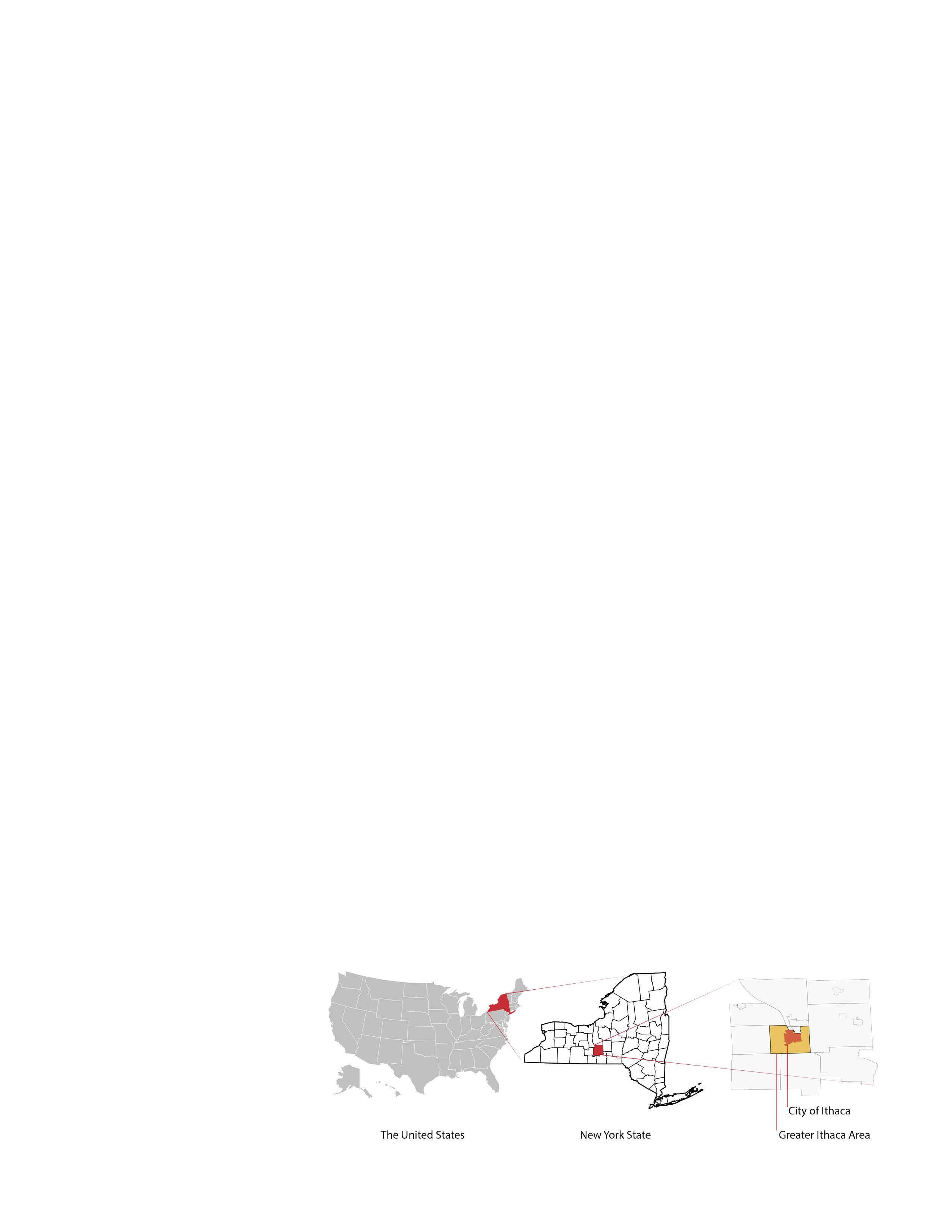
The study area - Greater Ithaca -includes several adjacent neighborhoods around the Town of Ithaca. The city of Ithaca is the seat of Tompkins County in New York State, its area is 5.39 mile² (2010). As of 2019 when the bike sharing data was collected, the population of the City of Ithaca is 30,837, of which 49.9% were female, 68.4% were white (U.S. Census Bureau QuickFacts, n.d.), and 87.8% were US citizens. With a student population of more than 20,000, Ithaca is home to Cornell University.

SVI, CV, and ML for measuring street built environment

Fig.1. Study area

Research Framework

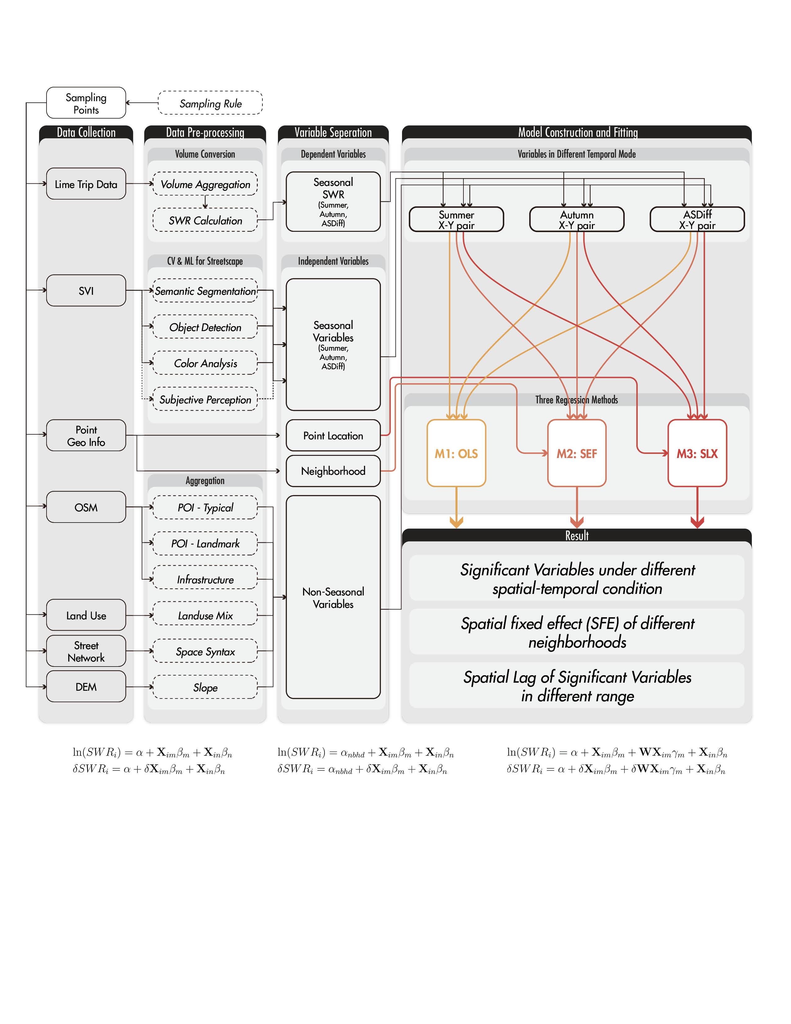
(1) Seasonal Weighted Rides (SWR) is calculated from the proportion of aggregated volume in a specific season on one road segment in total volume of all segments in this season.

For Summer and Autumn models, dependent variables are ln(SWR), the natural log of corresponding SWR; dependent variables are the combination of seasonal variables in corresponding season and non-seasonal variables.

For Autumn-Summer-Difference(ASDiff) model, dependent variables are the remainder of autumn ln(SWR) minus that of summer; dependent variables are the combination of remainder of autumn seasonal variables minus that of summer, and non-seasonal variables.

Ordinary Least Square(OLS) model does not consider spatial relationship (assuming variables as i.i.d.)

Spatial Fixed Effect(SFE) gives unique constant to points within a same neighborhood.

Spatial Lag of X (SLX) helps describe how other points in a set nearest range (the spatial weighted matrix is calculated with KNN) would affect current point.

Fig.2. Analytical framework

Data and Methodology

3.1

Dependent variable:

Seasonal Weighted Rides (SWR)

Data Validation

The DBS trips data in this research is provided by Lime. The dataset was collected from mobile phones with enabled AUTO-GPS function through the Lime app. A validation process went through to remove the following raw records:

(1) trips that started or end outside the Greater Ithaca area,

(2) trips whose distances were shorter than the length of a city block in Ithaca(0.05mi or 264ft) ,

(3) trips with too short or long duration.

Finally, 102,178 trip records were left.

Then, based on the method developed by Qiu & Chang, 2021, road central lines were deconstructed into several road segments interrupted by any kind of intersection of roads or routes.

Points Sampling

Segments are selected:

Total Volume ≥ 500; and Length ≥ 25m

Points are sampled:

8m offset from vertex; and 25m sampling distance

1170 Points on 452 Segments

Plot

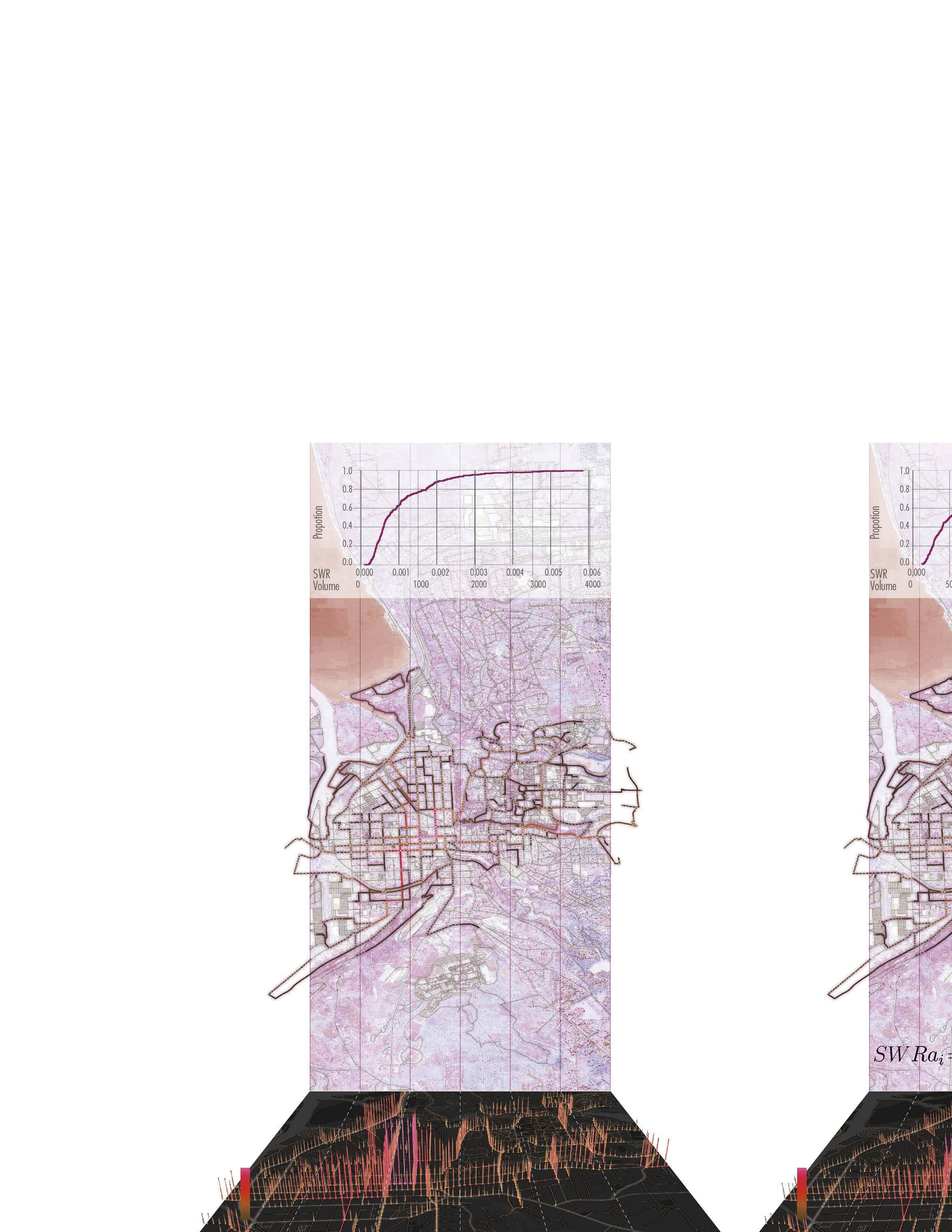
1170 Points 452 Segments

SWR Conversion

SWR Conversion

CDF Plot

CDF

SWR Conversion

Seasonal Weighted Rides captures how popular a segment is in this season.

Seasonal Difference Calculation

For single season models, X in CDF plot is SWR/Aggregated Volume of DBS ridership in that season.

For Seasonal Difference model, X in CDF plot is (autumn SWR - summer SWR)

Similar for other seasonal variables in the seasonal difference mode, including SWR as dependent variable, streetscape segmentation and object detection result in the independent variables.

CDF Plot

Cumulative Distribution Function is the probabilities that volume of a random segment is less than or equal to X (reveals the distribution of volume on road segments.)

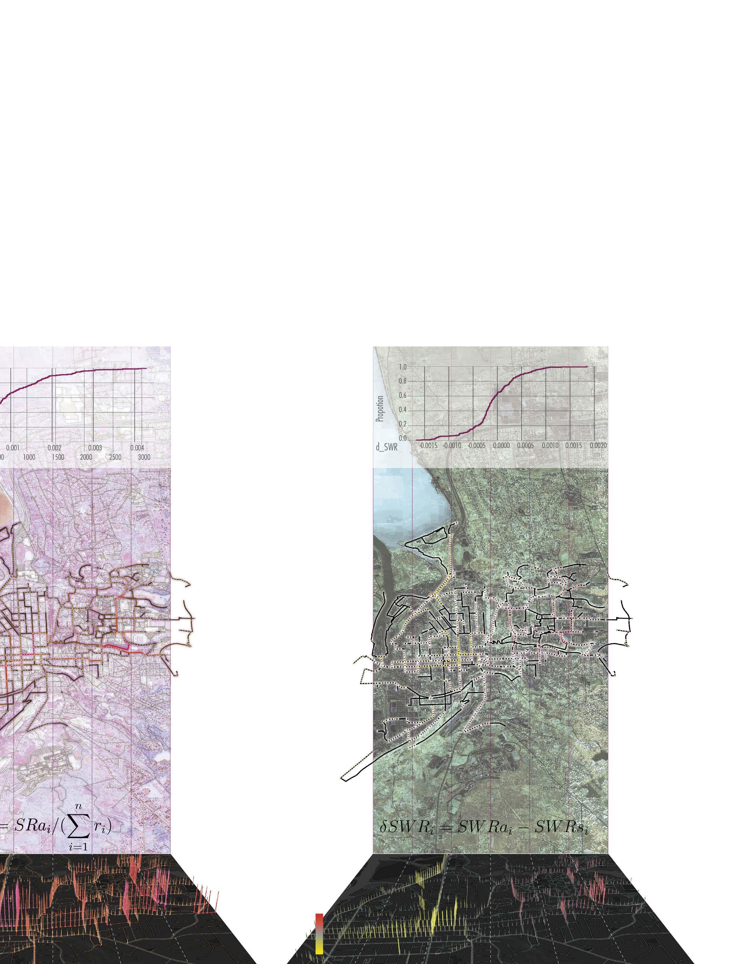
1170

Data and Methodology

3.2

Inependent variable: SVI and Visual

3.2.1

Object Detection and Semantic Segmentation

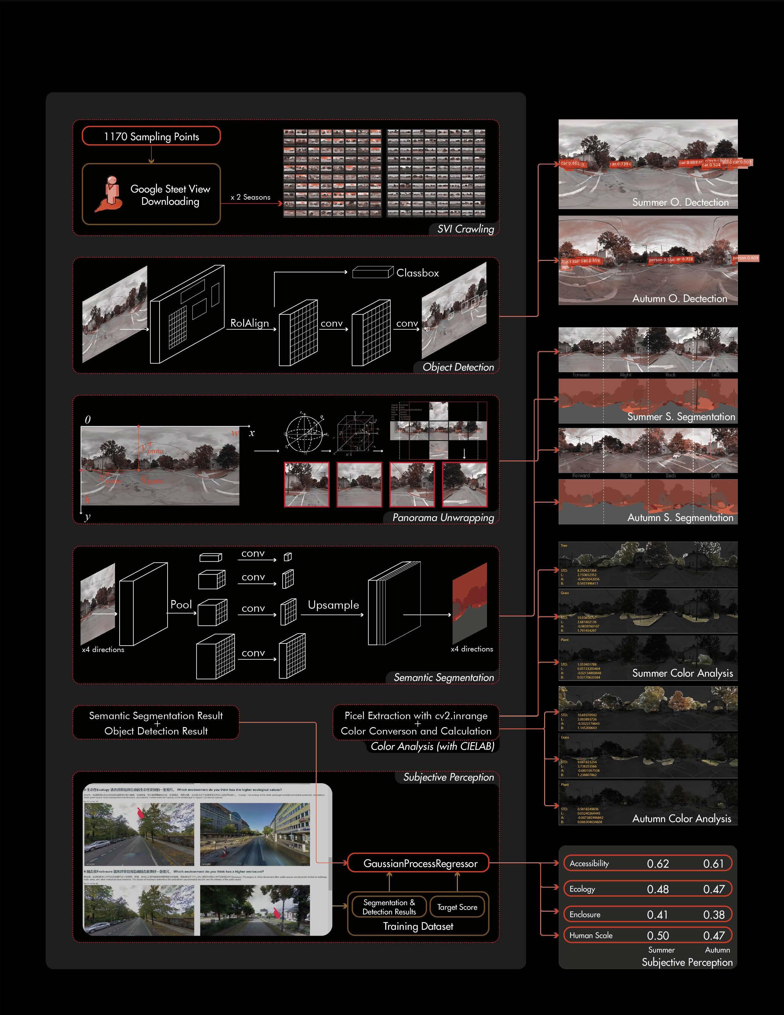
We traverse all Google Street View (GSV) taken in all seasons for all these sampling points, but only got GSV in summer (Jun, July, Aug) and fall (Sept, Oct, Nov). 1,170 sampling points that have GSV in both seasons finally remained.

We use Pyramid Scene Parsing Network (PspNet) (H. Zhao et al., 2017) under the open source deep learning framework MXNet in the GluonCV to conduct image segmentation, witha specific pre-trained model psp_resnet101_ade. To avoid potential distortion near the top and button of a panorama image, we use the py360convert package to unwarp the panorama into images in 6 directions before semantic segmentation.

3.2.2

Color Space Analysis

of humans). This dataset is collected from expert panel by a crowdsourcing visual survey). The dataset includes a set of view indices extracted from SVI (as input explanatory variables) and the corresponding perceptual scores（as output labels）. We split the dataset by 75% (225) and 25% (75) for training and testing purposes.

3.2.3

Subjective Measure of streetscape

of humans). This dataset is collected from expert panel by a crowdsourcing visual survey). The dataset includes a set of view indices extracted from SVI (as input explanatory variables) and the corresponding perceptual scores（as output labels）. We split the dataset by 75% (225) and 25% (75) for training and testing purposes.

of humans). This dataset is collected from expert panel by a crowdsourcing visual survey). The includes a set of view indices extracted from SVI (as input explanatory variables) and the corresponding perceptual scores（as output labels）. We split the dataset by 75% (225) and 25% (75) for training testing purposes.

In this paper, we use CIELAB to understand a general tendency of color (and its change) of street plants from urban cyclists’ perspective. Here we first extracted pixels that are identified as “Tree” from PspNet. Then we used the color convert function under python-colormath library to transform the color space of these pixels from RGB to CIELAB, calculated the average L, A, and B values in CIELAB color space, and the overall standard deviation of difference between the actual value the and average value.

We choose multiple ML algorithms which included K-Nearest Neighbors (KNN), Support Vector Machine (SVM), Random Forest (RF), Gaussian Process (GP), Gradient Boosting Regression (GB), ADA boost, and Bagging Regression, to predict the seven perceptions. Those algorithms are classical and mature in supervised learning. In urban related studies, they have been extensively used as a baseline in the prediction of a numerical target feature based on other features of an instance and have shown effectiveness and robustness (Naik et al., 2014; Safat et al., 2021; Zhang et al., 2018). Prediction results are compared by the balance performance judged by R-squared (R2), Mean Absolute Error (MAE), and Root Mean Square Error (RMSE). The training result can be found in Appendix 1. On average, GP is the optimal model for predicting the target dataset as a whole, and we used the Gaussian Process Regression method in Sklearn to learn the mapping from streetscape elements to perception, and apply the model to get the prediction of target perception scores.

of humans). This dataset is collected from expert panel by a crowdsourcing includes a set of view indices extracted from SVI (as input explanatory perceptual scores（as output labels）. We split the dataset by 75% (225) testing purposes.

of humans). This dataset is collected from expert panel by a crowdsourcing visual survey includes a set of view indices extracted from SVI (as input explanatory variables) and the perceptual scores（as output labels）. We split the dataset by 75% (225) and 25% (75) testing purposes.

In this research, we used the ML-based framework developed by related research (Qiu et al., 2023; Su et al., 2023; Xu et al., 2022) to evaluate the subjective perceptions score of the streetscape from street elements.

We use a dataset of 300 pre-labeled points to predict these perception scores: (1) Accessibility, (2) Ecology, (3) Enclosure, (4) Scale. The dataset includes a set of view indices extracted from SVI (as input explanatory variables) and the corresponding perceptual scores (as output labels). We split the dataset by 75% (225) and 25% (75) for training and testing purposes.

We choose multiple ML algorithms which included K-Nearest Neighbors (KNN), Support Vector Machine (SVM), Random Forest (RF), Gaussian Process (GP), Gradient Boosting Regression (GB), ADA boost, and Bagging Regression, to predict the seven perceptions. Those algorithms are classical and mature in supervised learning. In urban related studies, they have been extensively used as a baseline in the prediction of a numerical target feature based on other features of an instance and have shown effectiveness and robustness (Naik et al., 2014; Safat et al., 2021; Zhang et al., 2018). Prediction results are compared by the balance performance judged by R-squared (R2), Mean Absolute Error (MAE), and Root Mean Square Error (RMSE). The training result can be found in Appendix 1. On average, GP is the optimal model for predicting the target dataset as a whole, and we used the Gaussian Process Regression method in Sklearn to learn the mapping from streetscape elements to perception, and apply the model to get the prediction of target perception scores.

Measuring the seasonal variations of associations between streetscape and dockless bikeshare trip volume

Measuring the seasonal variations of associations between streetscape and dockless bikeshare trip volume

Measuring the seasonal variations of associations between streetscape and dockless bikeshare trip volume

Measuring the seasonal variations of associations between streetscape and dockless bikeshare trip volume

Measuring the seasonal variations of associations between streetscape and dockless bikeshare trip volume

Measuring the seasonal variations of associations between streetscape and dockless bikeshare trip volume

We choose multiple ML algorithms which included K-Nearest Neighbors (KNN), Support Vector Machine (SVM), Random Forest (RF), Gaussian Process (GP), Gradient Boosting Regression (GB), ADA boost, and Bagging Regression, to predict the seven perceptions. Those algorithms are classical and mature in supervised learning. On average, GP is the optimal model for predicting the target dataset as a whole, and we used the Gaussian Process Regression method in Sklearn to learn the mapping from streetscape elements to perception, and apply the model to get the prediction of target perception scores.

We choose multiple ML algorithms which included K-Nearest Neighbors (KNN), Support Machine (SVM), Random Forest (RF), Gaussian Process (GP), Gradient Boosting Regression (GB), boost, and Bagging Regression, to predict the seven perceptions. Those algorithms are classical mature in supervised learning. In urban related studies, they have been extensively used as a baseline the prediction of a numerical target feature based on other features of an instance and have effectiveness and robustness (Naik et al., 2014; Safat et al., 2021; Zhang et al., 2018). Prediction are compared by the balance performance judged by R-squared (R2), Mean Absolute Error (MAE), Root Mean Square Error (RMSE). The training result can be found in Appendix 1. On average, optimal model for predicting the target dataset as a whole, and we used the Gaussian Process Regression method in Sklearn to learn the mapping from streetscape elements to perception, and apply the get the prediction of target perception scores.

Appendix

Appendix

Appendix

Appendix

Appendix

Appendix

Table 1. Performance of GaussianProcessRegressor (GP) predictions.

We choose multiple ML algorithms which included K-Nearest Neighbors Machine (SVM), Random Forest (RF), Gaussian Process (GP), Gradient boost, and Bagging Regression, to predict the seven perceptions. Those mature in supervised learning. In urban related studies, they have been the prediction of a numerical target feature based on other features effectiveness and robustness (Naik et al., 2014; Safat et al., 2021; Zhang are compared by the balance performance judged by R-squared (R2), Mean Root Mean Square Error (RMSE). The training result can be found in Appendix optimal model for predicting the target dataset as a whole, and we used method in Sklearn to learn the mapping from streetscape elements to percepti get the prediction of target perception scores.

We choose multiple ML algorithms which included K-Nearest Neighbors (KNN), Machine (SVM), Random Forest (RF), Gaussian Process (GP), Gradient Boosting Regression boost, and Bagging Regression, to predict the seven perceptions. Those algorithms mature in supervised learning. In urban related studies, they have been extensively used the prediction of a numerical target feature based on other features of an instance effectiveness and robustness (Naik et al., 2014; Safat et al., 2021; Zhang et al., 2018). Prediction are compared by the balance performance judged by R-squared (R2), Mean Absolute Error Root Mean Square Error (RMSE). The training result can be found in Appendix 1. On average, optimal model for predicting the target dataset as a whole, and we used the Gaussian Process method in Sklearn to learn the mapping from streetscape elements to perception, and apply get the prediction of target perception scores.

Appendix 1. ML model performance

Appendix 1. ML model performance

Appendix 1. ML model performance

Appendix 1. ML model performance

Appendix 1. ML model performance

The results discussed in this section (semantic segmentation, objection detection, color analysis, and objective perception) are seasonal variables and will be fitted in their corresponding seasonal model. Additionally, we compute the seasonal difference for these seasonal variables with Eq. (4).

Appendix 1. ML model performance

Table 1. Performance of GaussianProcessRegressor (GP)

Table 1. Performance of GaussianProcessRegressor (GP) predictions.

3.3.2.5 Data in models

3.3.2.5 Data in models

3.3.2.5 Data in models

3.3.2.5 Data in models

3.3.2.5 Data in models

We tried commonly used machine learning models, including Even though for Accessibility ADA boost (R2=0.42) and Bagging Regression(R2=0.42) had better R2 than GP(R2=0.4), for Enclosure Decision Tree (R2=0.54) had better R2 than GP(R2=0.53), and for Scale RF(R2=0.44) and GB(R2=0.42) had better R2 than GP(R2=0.39), GP had acceptable R2 (range from 0.39-0.53) for all perception scores, and outperformed all other models in very low RMSE(range from 0.16 to 0.18) and MAE(range from 0.13 to 0.15).

We tried commonly used machine learning models, including Even though for Accessibility ADA boost (R2=0.42) and Bagging Regression(R2=0.42) had better R2 than GP(R2=0.4), for Enclosure Decision Tree (R2=0.54) had better R2 than GP(R2=0.53), and for Scale RF(R2=0.44) and GB(R2=0.42) had better R2 than GP(R2=0.39), GP had acceptable R2 (range from 0.39-0.53) for all perception scores, and outperformed all other models in very low RMSE(range from 0.16 to 0.18) and MAE(range from 0.13 to 0.15).

The results discussed in this section (semantic segmentation, objection detection, color analysis, and objective perception) are seasonal variables and will be fitted in their corresponding seasonal model. Additionally, we compute the seasonal difference for these seasonal variables with Eq. (3).

We tried commonly used machine learning models, including Even though for Accessibility ADA boost (R2=0.42) and Bagging Regression(R2=0.42) had better R2 than GP(R2=0.4), for Enclosure Decision Tree (R2=0.54) had better R2 than GP(R2=0.53), and for Scale RF(R2=0.44) and GB(R2=0.42) had better R2 than GP(R2=0.39), GP had acceptable R2 (range from 0.39-0.53) for all perception scores, and outperformed all other models in very low RMSE(range from 0.16 to 0.18) and MAE(range from 0.13 to 0.15).

We tried commonly used machine learning models, including Even though for Accessibility ADA boost (R2=0.42) and Bagging Regression(R2=0.42) had better R2 than GP(R2=0.4), for Enclosure Decision Tree (R2=0.54) had better R2 than GP(R2=0.53), and for Scale RF(R2=0.44) and GB(R2=0.42) had better R2 than GP(R2=0.39), GP had acceptable R2 (range from 0.39-0.53) for all perception scores, and outperformed all other models in very low RMSE(range from 0.16 to 0.18) and MAE(range from 0.13 to 0.15).

We tried commonly used machine learning models, including Even though for Accessibility ADA boost (R2=0.42) and Bagging Regression(R2=0.42) had better R2 than GP(R2=0.4), for Enclosure Decision Tree (R2=0.54) had better R2 than GP(R2=0.53), and for Scale RF(R2=0.44) and GB(R2=0.42) had better R2 than GP(R2=0.39), GP had acceptable R2 (range from 0.39-0.53) for all perception scores, and outperformed all other models in very low RMSE(range from 0.16 to 0.18) and MAE(range from 0.13 to 0.15).

We tried commonly used machine learning models, including Even though for Accessibility ADA boost (R2=0.42) and Bagging Regression(R2=0.42) had better R2 than GP(R2=0.4), for Enclosure Decision Tree (R2=0.54) had better R2 than GP(R2=0.53), and for Scale RF(R2=0.44) and GB(R2=0.42) had better R2 than GP(R2=0.39), GP had acceptable R2 (range from 0.39-0.53) for all perception scores, and outperformed all other models in very low RMSE(range from 0.16 to 0.18) and MAE(range from 0.13 to 0.15).

The results discussed in this section (semantic segmentation, objection detection, color analysis, and objective perception) are seasonal variables and will be fitted in their corresponding seasonal model. Additionally, we compute the seasonal difference for these seasonal variables with Eq. (3).

The results discussed in this section (semantic segmentation, objection detection, color and objective perception) are seasonal variables and will be fitted in their corresponding seasonal Additionally, we compute the seasonal difference for these seasonal variables with Eq. (3).

We tried commonly used machine learning models, including for Accessibility ADA boost (R2=0.42) and Bagging Regression(R2=0.42) had better R2 than GP(R2=0.4), for Enclosure Decision Tree (R2=0.54) had better R2 than GP(R2=0.53), and for Scale RF(R2=0.44) and GB(R2=0.42) had better R2 than GP(R2=0.39), GP had acceptable R2 (range from 0.39-0.53) for all perception scores, and outperformed all other models in very low RMSE(range from 0.16 to 0.18) and MAE(range from 0.13 to 0.15).

The results discussed in this section (semantic segmentation, objection and objective perception) are seasonal variables and will be fitted in their Additionally, we compute the seasonal difference for these seasonal variables

(4)

The results discussed in this section (semantic segmentation, objection detection, and objective perception) are seasonal variables and will be fitted in their corresponding Additionally, we compute the seasonal difference for these seasonal variables with Eq. (3).

�������� ������������������������ = �������������������������������� �������� ������������������������ (4)

Here, for sampling point �������� ,

Here, for sampling point �������� , �������������������������������� is autumn results of seasonal variables, �������������������������������� is autumn results of seasonal variables, and �������� ������������������������ is the difference between autumn and summer seasonal variables.

Here, for sampling point

Eq. (4). Here, for sampling point , is autumn results of seasonal variables, is autumn results of seasonal variables, and is the difference between autumn and summer seasonal variables.

results of seasonal variables, �������������������������������� is autumn results of seasonal variables, and ��������

is autumn results of seasonal variables, �������������������������������� is autumn of seasonal variables, and �������� ������������������������ is the difference between autumn and summer seasonal variables.

3.3.3 POI, landmark, and infrastructure

Here, for sampling point

3.3.3 POI, landmark, and infrastructure

is the difference between autumn and summer seasonal variables.

results of seasonal variables,

�������� ������������������������ = �������������������������������� �������� ������������������������ Here, for sampling point �������� , �������������������������������� is autumn results of seasonal variables, of seasonal variables, and �������� ������������������������ is the difference between autumn and summer

3.3.3 POI landmark and infrastructure

is the difference between autumn and summer seasonal

is of seasonal variables, and

Here we assume that POIs, landmark, and infrastructure would not change too much

3.3.3 POI landmark and infrastructure

Table 1. Performance of GaussianProcessRegressor (GP) and other ML predictions.

Table 1. Performance of GaussianProcessRegressor (GP) predictions.

Data and Methodology

Inependent variable: Non-Visual

3.2.1

3.2.2

3.2.3

3.3 3.4

Object Detection and Semantic Segmentation

Color Space Analysis

Subjective Measure of streetscape

Visual Variable summary

We capture different types of POIs within a 500m radius buffer of each sampling point. We also take into account landmark-like destinations, which are unique in the city and can be attractive at different distances for people. To capture these, the buffer zone radius for these landmarks is set to 1000m (typical 5 min rides on a bicycle) and 3000m (typical 15 min rides on a bicycle).

For infrastructure information, we choose number of transit facility, bicycle parking, traffic signals, and type of road. The buffer radius is set to 100m.

Land use is a common data source in bike studies to learn about the built environment context (Krenn et al., 2014; Ma et al., 2020; Noland et al., 2016). We used formula derived from the Shannon Index which can capture the entropy of data in a given set.

From USGS we download high resolution(1-meter) Digital Elevation Model (DEM). To reduce interference from potential outlier on the slope raster map, we use the medium slope within 5 meters forward and backward of each sampling point.

Appendix 2. Data Description

Street network, as a way to demonstrate the structure of the built environment is another aspect influencing cyclists’ behavior. After calculating the VIF we remove space syntax score with high multicollinearity (VIF>10), and finally choose Connectivity, Normalized Angular Choice (Nach), and Angular Integration (with segment length weighted, or SLW). Nach and Angular Integration(SLW) both have two radius: 250m and 1000m.

Appendix Table 2.1 Description of seasonal variables of summer (for model M1_Summer, M2_Summer, M3_Summer, M4_Summer)

Table 2 Description of seasonal variables of summer (for model M1_Summer, M2_Summer, M3_Summer, M4_Summer).

数据和方法

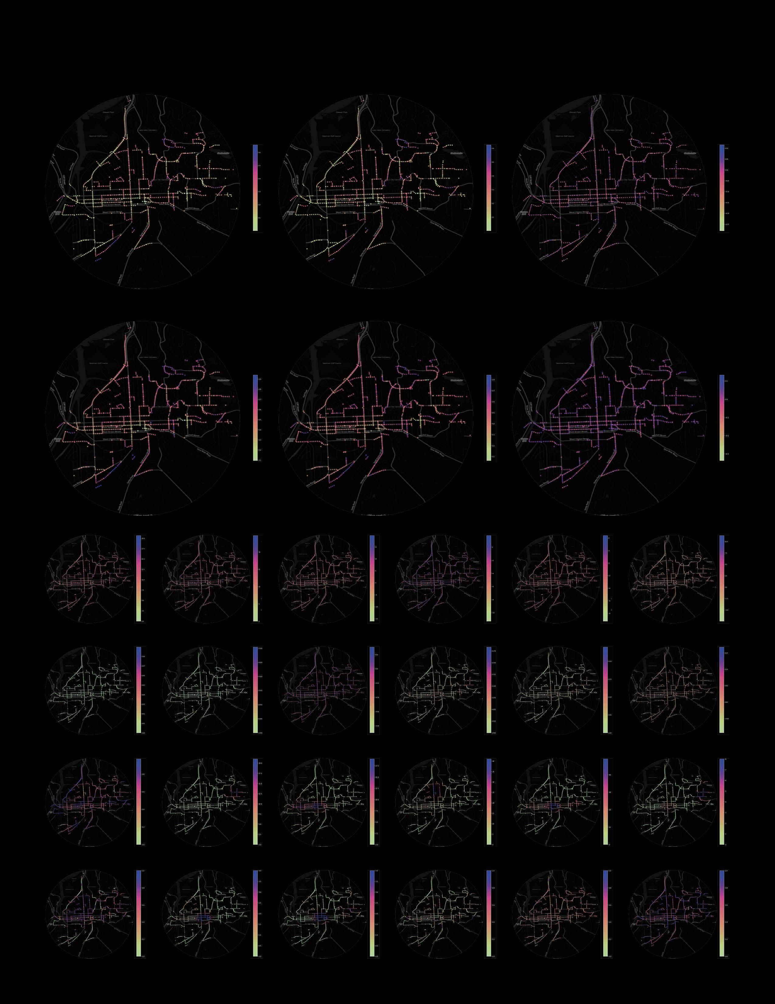
tree_lab_a (Autumn) POI

tree_lab_a (ASDiff)

POI

5.1

Model result and discussion

car, road, sidewalk, water, wall, grass color deviation, tree color deviation, tree LAB a value, and nonseasonal variables such as land use mix score. (2) some variables show their significance for the first time, this applies to variables such as number of education POI. (3) for landmark variables, some are no longer significant while some start to be. (4) street network variables maintain their significance (5) the terrain factor continues to be insignificant in all 6 models up to now.

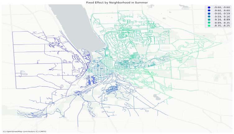
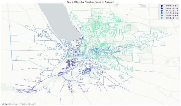
Fig. 10 shows the spatial fixed effect by neighborhood in summer and autumn and Table 5 shows the neighborhood ranking of fixed effect. The lower the SFE is, the lower the inherent attractiveness of the neighborhood is, and the harder it is to witness a ride in this neighborhood. For spatial fixed effects value, spatial fixed effects of most neighborhoods in autumns are lower than that in summer, except Downtown, South Hill and West Hill. For spatial fixed effects ranking, it’s very consistent between summer and autumn for the top seven neighborhoods, North Campus/Northeast and Maplewood/East Hill are the two easiest neighborhoods to witness a ride for both seasons, while North Campus/Northeast being highest in autumn and Maplewood/East Hill in summer. Similar consistency also applies to 8th to 13th neighborhoods, with the only exception being 8th and 13th. IFM/Stewart Park being 8th in summer has only 13th in autumn, and West Hill vice versa. These two can be considered as “seasonal neighborhoods”.

The regression diagnosis results indicate that: (1) Autumn models have higher R2 than Summer models, suggesting that our current variables lack more summer information that can explain the dependent variables than autumn information, regardless of whether this information is seasonal or not. (2) ASDiff models outperform both Autumn and Summer models under the same regression method, indicating that the difference in seasonal variables between summer and autumn can better explain the seasonal change in bike sharing. (3) Model 2 shows improved explanatory power compared to Model 1, demonstrating the effectiveness of subjective human-perceived streetscape features in enhancing prediction ability (4) Incorporating spatial fixed effects significantly improves the performance of all three models, which support our previous assumption that a systematic neighborhood “unevenness” could impact DBS usage in Ithaca.

car, road, sidewalk, water, wall, grass color deviation, tree color deviation, tree LAB a value, and nonseasonal variables such as land use mix score. (2) some variables show their significance for the first time, this applies to variables such as number of education POI. (3) for landmark variables, some are no longer significant while some start to be. (4) street network variables maintain their significance (5) the terrain factor continues to be insignificant in all 6 models up to now.

Fig. 10 shows the spatial fixed effect by neighborhood in summer and autumn and Table 5 shows the neighborhood ranking of fixed effect. The lower the SFE is, the lower the inherent attractiveness of the neighborhood is, and the harder it is to witness a ride in this neighborhood. For spatial fixed effects value, spatial fixed effects of most neighborhoods in autumns are lower than that in summer, except Downtown, South Hill and West Hill. For spatial fixed effects ranking, it’s very consistent between summer and autumn for the top seven neighborhoods, North Campus/Northeast and Maplewood/East Hill are the two easiest neighborhoods to witness a ride for both seasons, while North Campus/Northeast being highest in autumn and Maplewood/East Hill in summer. Similar consistency also applies to 8th to 13th neighborhoods, with the only exception being 8th and 13th. IFM/Stewart Park being 8th in summer has only 13th in autumn, and West Hill vice versa. These two can be considered as “seasonal neighborhoods”.

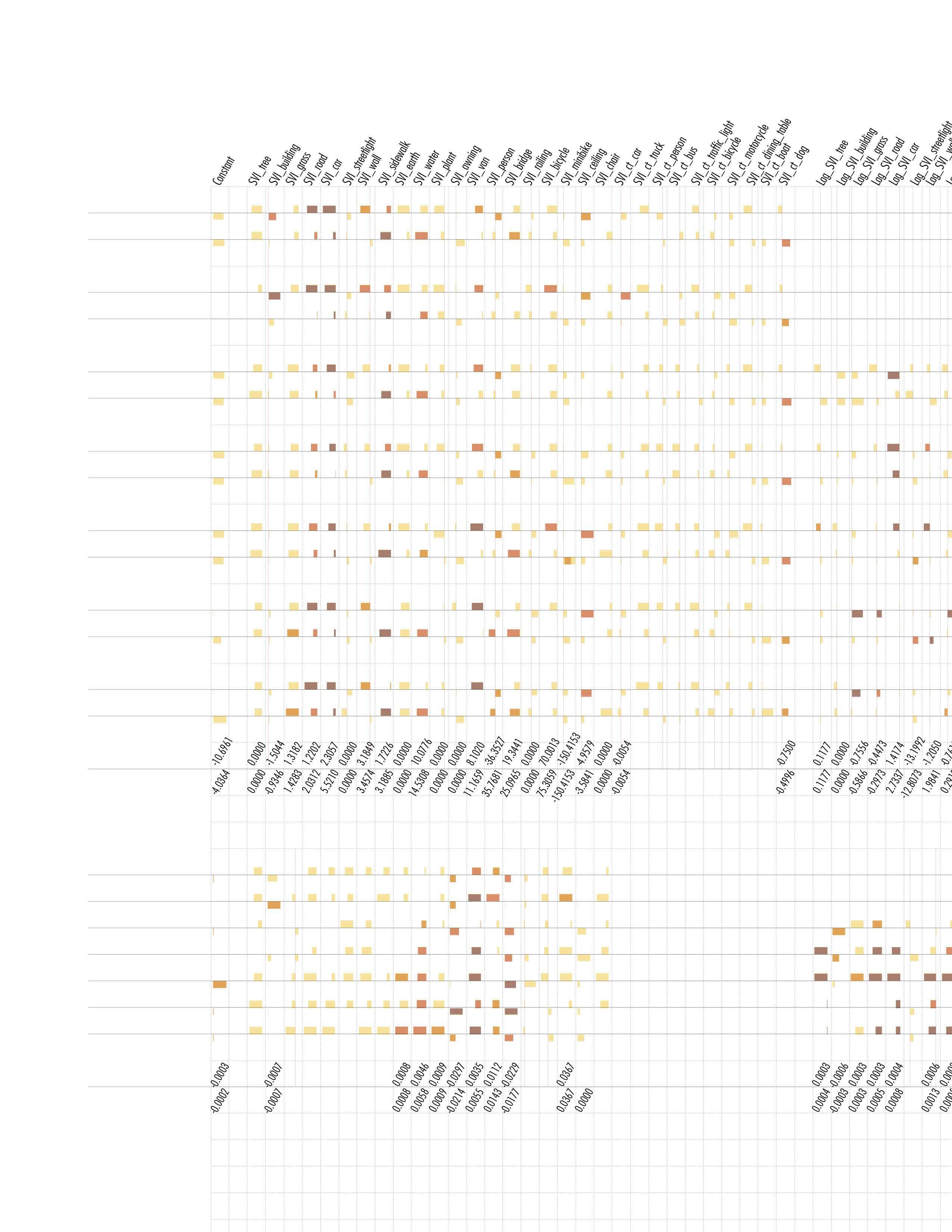
Most significant variables in at least one season keep their sign in another, and all significant variables in both seasons keep same sign. Many variables show consistent significance in summer and autumn, such as visual ratio of tree, road, car, sidewalk, water, lab b value of tree color, grass color diversion, Number of commercial POI, land use mix score, typical Landmark POI, Connectivity, Normalized Angular Choice and integration degree of the road network. Some variables only show significance in only one season, such as visual ratio of building, wall in summer, and tree color deviation and LAB value of tree and grass color in autumn.

4.5 SLX model regression results

The completed SFE model result can be found in Appendix 5-1 and Appendix 5-2

Taking the spatial lag of x into account would improve model performance significantly. While some variables are consistent in their coefficient and significance across different models, some show inconsistency when different spatial effects or observation ranges With the addition of seasonal different model, some variables reveal their hidden significance in making seasonal cycling different.

It’s very consistent for the top seven and 9th to 12th neighborhoods, with the only exception being 8th and 13th. IFM/Stewart Park being 8th in summer has only 13th in autumn, and West Hill vice versa. These two can be considered as “seasonal neighborhoods”. In terms of value, spatial fixed effects of most neighborhoods in autumns are lower than that in summer, except Downtown, South Hill and West Hill. The above result shows that spatial fixed effect in Ithaca is also sensitive to seasonal change.

4.5.1 Variables at current location within neighboring range

Noticeably, road, car, and sidewalk, are consistently significant locally at all ranges in both seasons, which is same as their performance in OLS and SFE. However, while their coefficient are close to what they have in OLS or SFE in a corresponding season and consistently positive, coefficient in SLX presents different pattern. Coefficient for road’s lag are increasing with observation range all the way from 2 to 30, car’s lag in both seasons reach a peak when k = 5, and sidewalk’s lag have a bottom at 5 (summer) and 10 (autumn). SLX also reveals a divergent significant range. For instance, ceiling, being significant in summer in both OLS and SFE models, is only significant at larger range in SLX.

Specifically, SLX models with the closer k value show similar significance and coefficient. For example, M4(k=5) and M4(k=2) or M4(k=10) have higher alignment than with other SLX models, so does M4(k=20) with M4(k=10) or M4(k=30). However, certain variables are not continuous in their significance across different neighboring ranges, like sidewalk which is significant in OLS, only shows significance when k=5; person only when k=20. Some variables will not be significant until k reaches a threshold value, road in autumn is significant in OLS, but in SLX it only starts to be significant until k reaches 10 and higher; nevertheless, ct_dog is no longer significant when k is larger than or equal to 20.

4.5.2 Variables within a neighboring range from the current location

First, some streetscape elements’ impact on SWR can be implicit in one single season, which is not shown in any of the single-season models but only in ASDiff models. Second, the addition of seasonal difference models greatly improves model performance at all modeling methods (OLS, SFE, and SLX). The fact that huge model improvement happens when SWR and seasonal independent variables are all replaced with their corresponding seasonal difference suggests that other variables we haven’t taken into the model might not be as important as what we have in current models in terms of explaining the seasonal change of bike sharing.

Significance and coefficient between models with the nearest k value are much less similar compared with variables at the current location, which means that variables within the neighboring range are more sensitive to change in the observation range. What’s more, variables within different neighboring ranges have shown a very diverse consistency pattern, which is not even close to what we observe at the current location.

The continued consistency that we discussed before still exists, but only van stays consistent across all observation ranges. Other consistent variables can only maintain their continued significance within limited ranges. For example, road and grass in summer when the observation range is large (k=20 and 30), car in summer when the observation range is small to medium large(k=2, 5 and 10), ct_traffic_light in

autumn when the observation range is not small(k=5,10,20, and 30), etc.

Table 4. SFE Neighborhood in Different Seasons.

Table 5. Fixed Effect of Neighborhood in Different Seasons Models (M2_Autumn and M2_Summer)

(a) Fixed effect by neighborhood in summer (b) Fixed effect by neighborhood in Autumn

Fig. 10 Spatial Fixed Effect result from SFE models in two seasons

Table 5. Fixed Effect of Neighborhood in Different Seasons Models (M2_Autumn and M2_Summer)

Modeling and Result

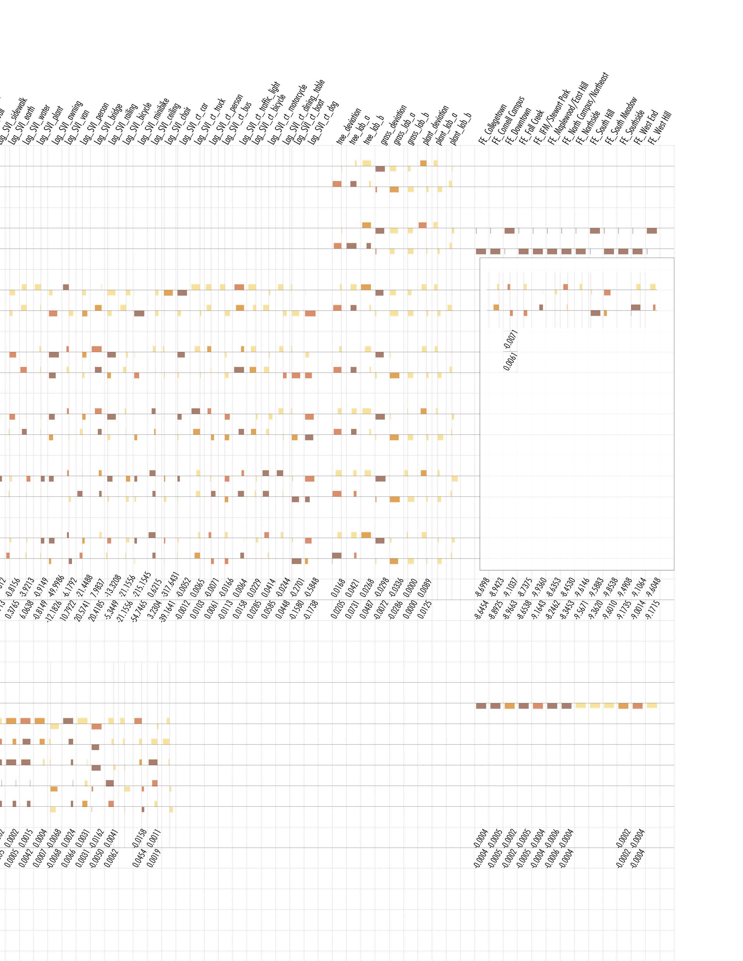
Notes & Label

d

j e c

j

g h i

a b f

P value Sign

a: 0.01≥p b: 0.05≥p≥0.01 c: 0.1≥p≥0.05 d: p≥0.1

e: Positive Coeff.

f: Negative Coeff.

g: Same variable has different sign in temporal mode

Magnitude

h: Maxium Coeff. in all temporal mode

i: Minimum Coeff. in all temporal mode

j: Width of cell is normalized magnitude in Coeff. range

Results *

Variables in different spatial modes

Certain variables are significant in one season across all spatial modes, like sidewalk and water in autumn; Certain variables are inconsistently significant in one season, like wall and ceiling in summer; Most variables are consistent at their sign of coeff.; SLX models shows the change of effective influence range of elements, which applies to bridge, ceiling, etc.

Variables in different temporal modes

ASDiff show that variables significant in single season models might not effective enough to make seasonal change, while some not significant in neither single season models actually influence seasonal behavior change.

C2

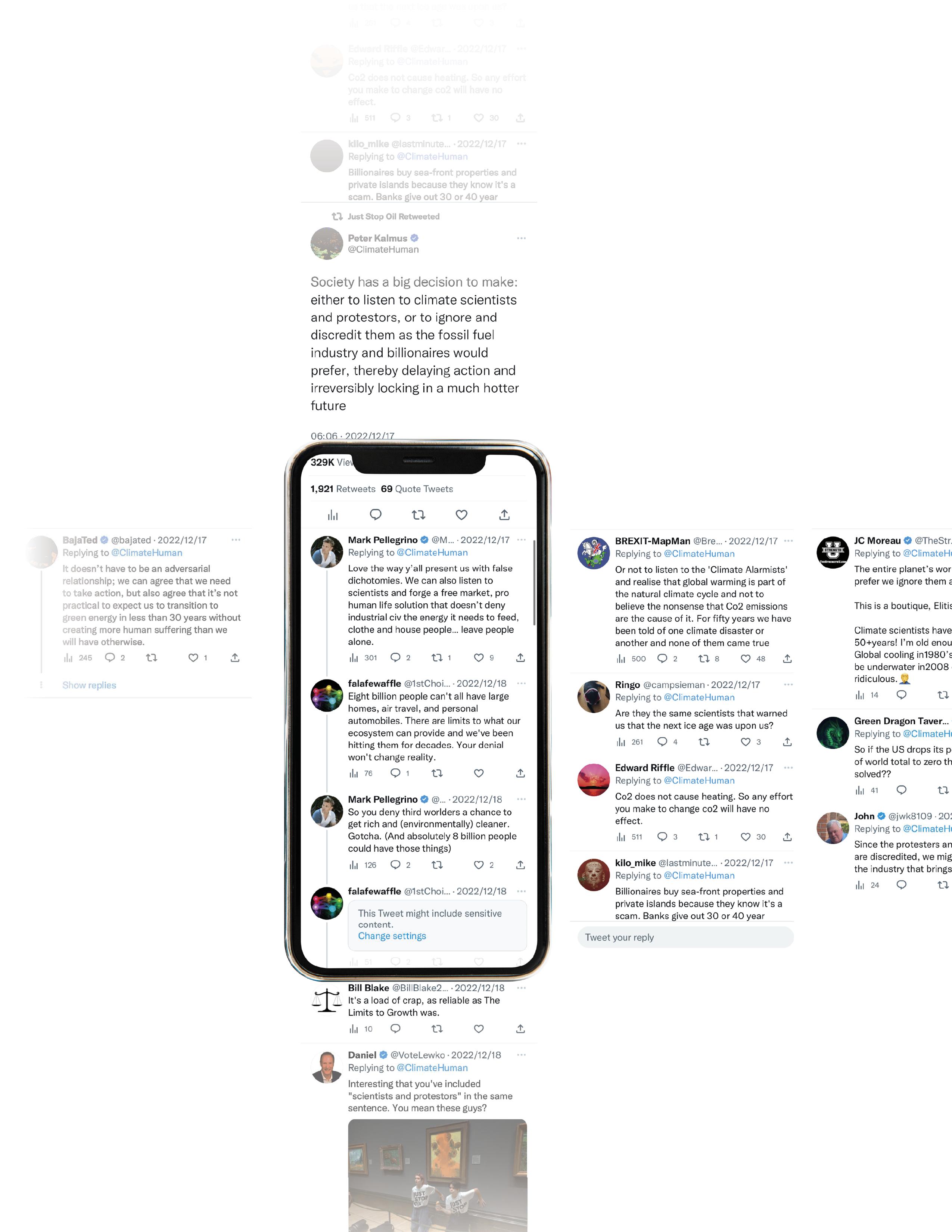
De-polarization: A Graph-based New Paradigm for Browsing and Sharing Experience in Social Media

How a topic is diffused, and how conversations and discussions would fall into echo chamber, over time?

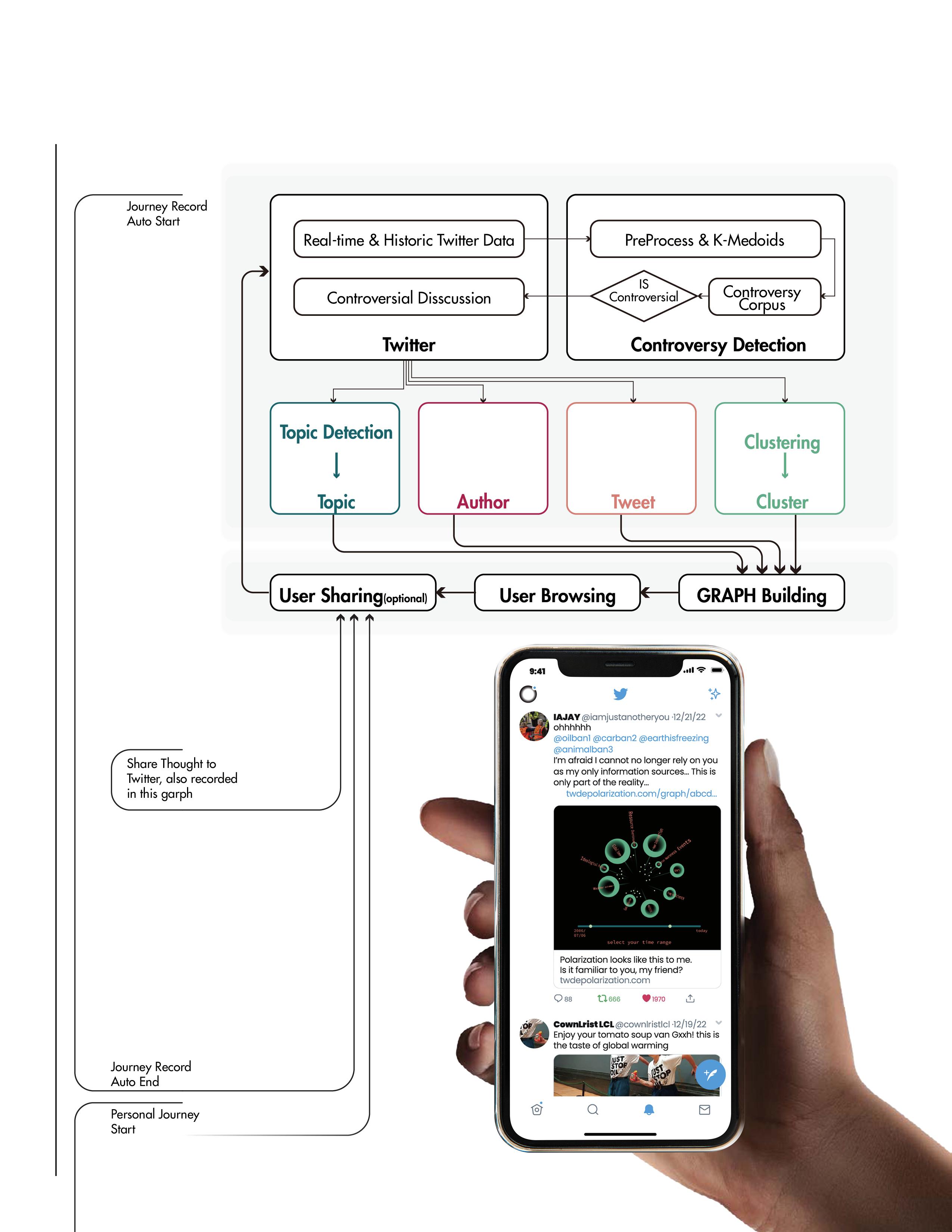
Built for the X (formerly Twitter), this design is a new kind of social media architecture to empower individuals’ information control, and a new kind of interface for browsing, reflection, and sharing.

The design of zoom levels displays different levels of detail and attribute of a topic, subtopic, emotion orientation, and even specific tweet. Users can overview the debates while sharing their browsing journey and other evoked thoughts.

The experience itself becomes a conversation between user and facts, based on cross scale facts and details. Thus, a new social media paradigm:

A rational and constructive data scape for people to embrace differences while cherish the common.

2022 Fall

Individual Research + Individual Design

NLP, graph, UI, clustering Media Skill

Kaggle Dataset+ Personal Processing, twarc, nltk, kmeans, keyBERT, Adobe Suites, Gephi, Figma

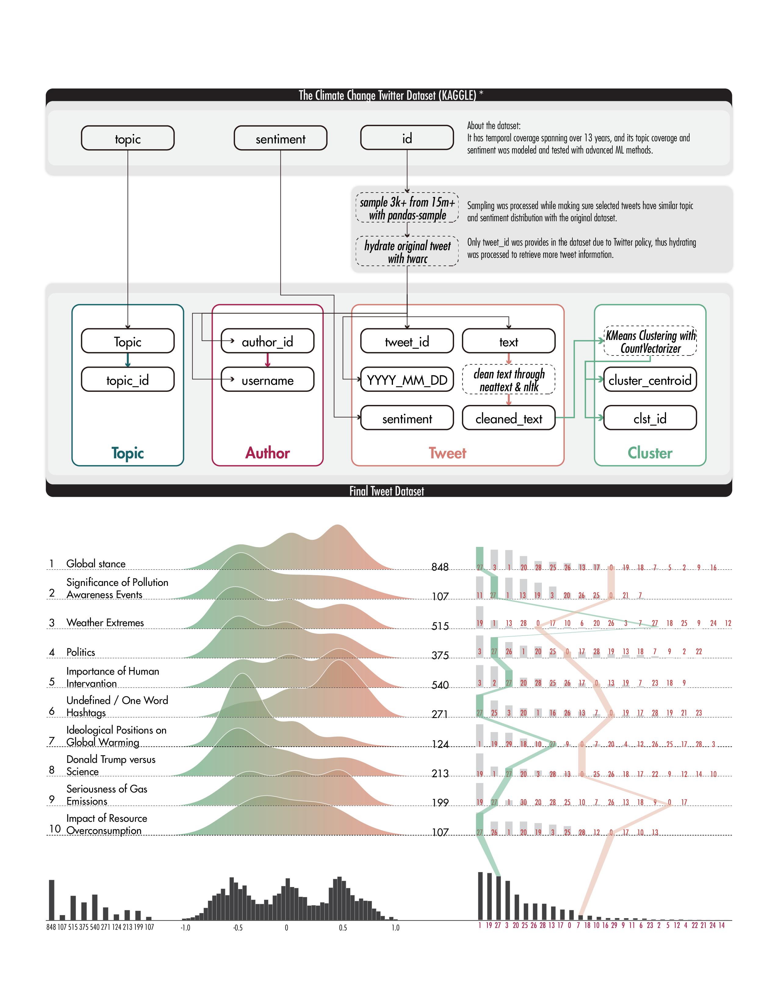
A New Type of Data Architecture: Store and Explore

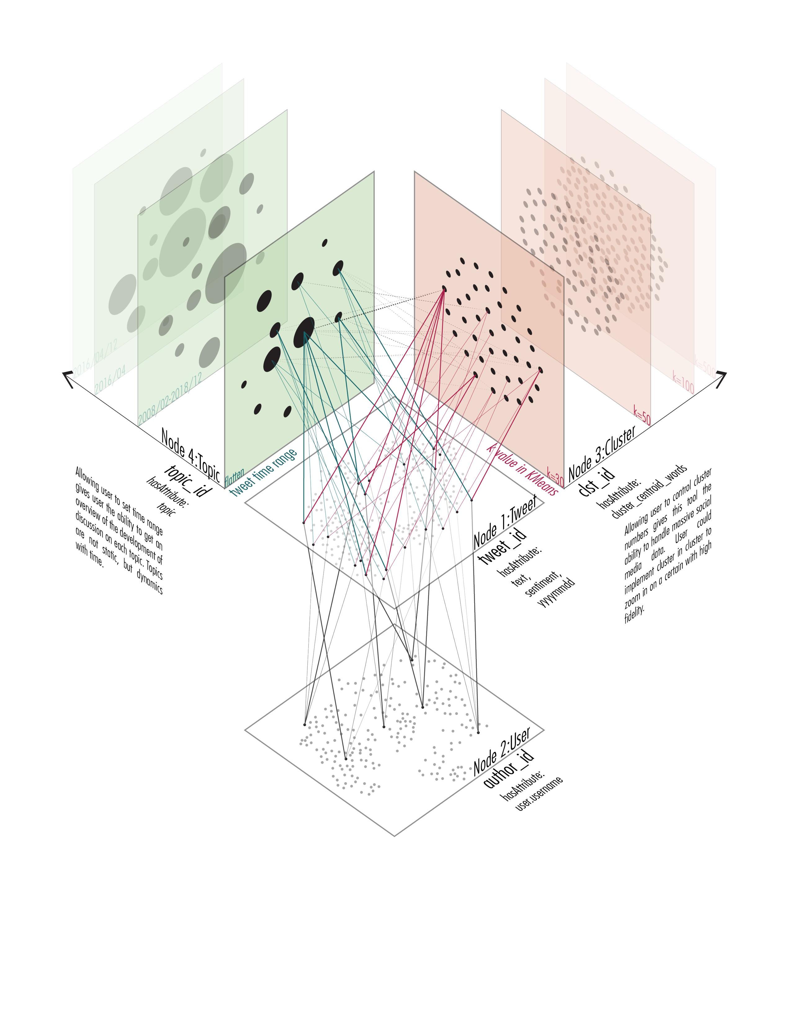
4 types of

4 types of Edge: Notes

Building edges between topic and cluster is essential to display complex discussion with high fidelity.

Tweets under one topic can be clustered in multiple cluster, user could then better navigates their journey in the datascape.

Zoom Level: Data Structure & Interface

ZOOM LEVEL 1

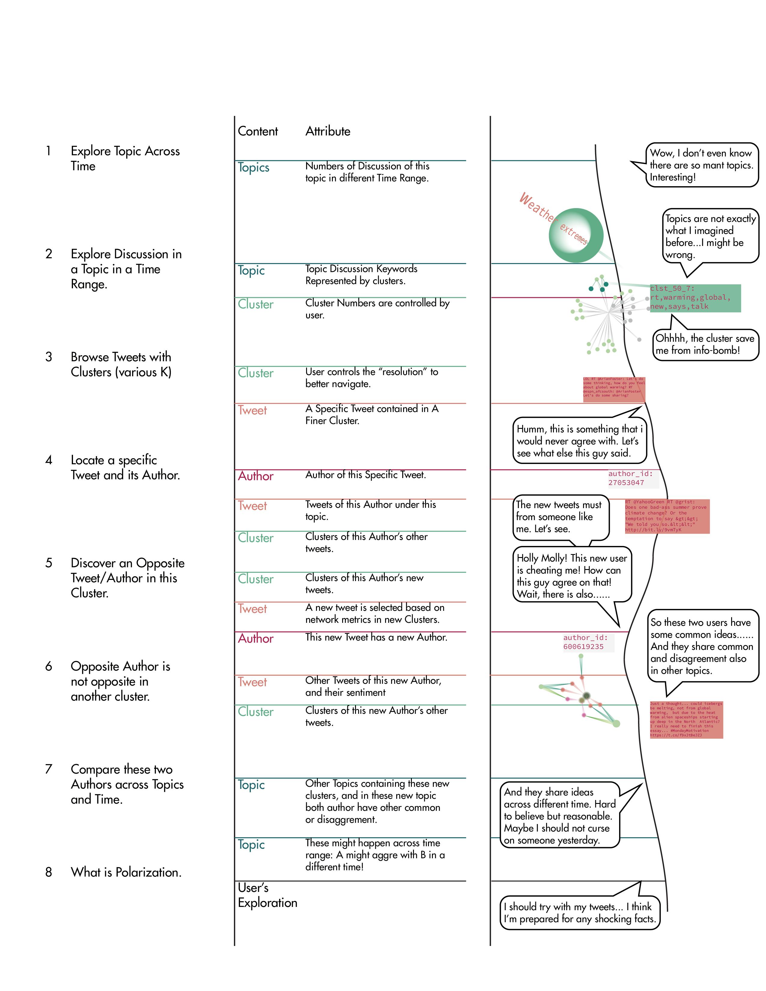
Explore Topic Across Time

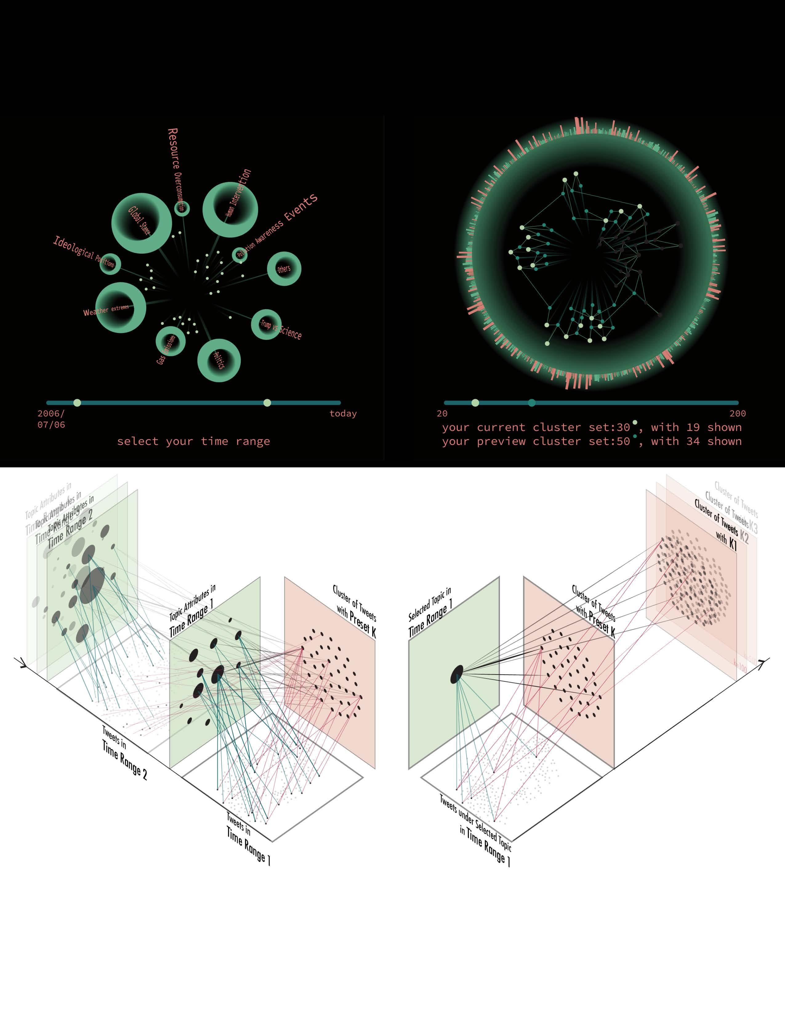
ZOOM LEVEL 2

Explore Discussion in a Topic in a Time Range.

Zoom Level: A1

Topics are evolving over time, a new topic can be popular in time range A but unfashionable in time range B. Thus, I design the first zoom level to allow user explore topic development throughout time. In the time range user selects, attributes like number of tweets under this topic, cluster detected with these tweets, are displayed in the interface.

After choosing a topic in a specific time range, user would explore the clusters to better navigate the browsing experience. Centroid point of cluster would provide keywords in a cluster. With the user continue the experiment on more finer clustering result, discussion in a cluster would have higher fidelity, providing more specific description of a content within a cluster.

ZOOM LEVEL 3

Browse Tweets with Clusters (various K)

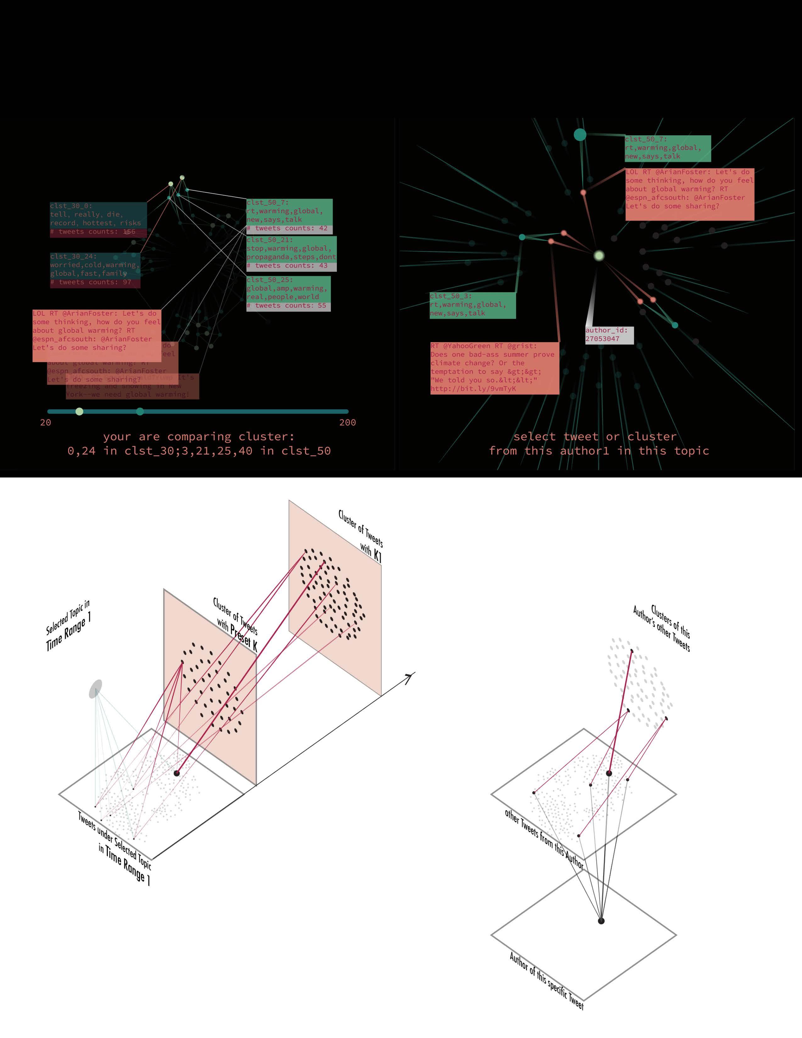
Continuing his/her exploration in the clusters, user would finally find a cluster with concrete information, and a limited number of tweets under this cluster.

ZOOM LEVEL 4

Locate a specific Tweet and its Author.

After choosing a specific tweet, more attributes of this tweet would pop up: author of this tweet, and other tweets from this author “author1” under the chosen topic in the chosen time range. And cluster (k is what the user set at last step) of the new tweets.

Zoom Level: Data Structure & Interface

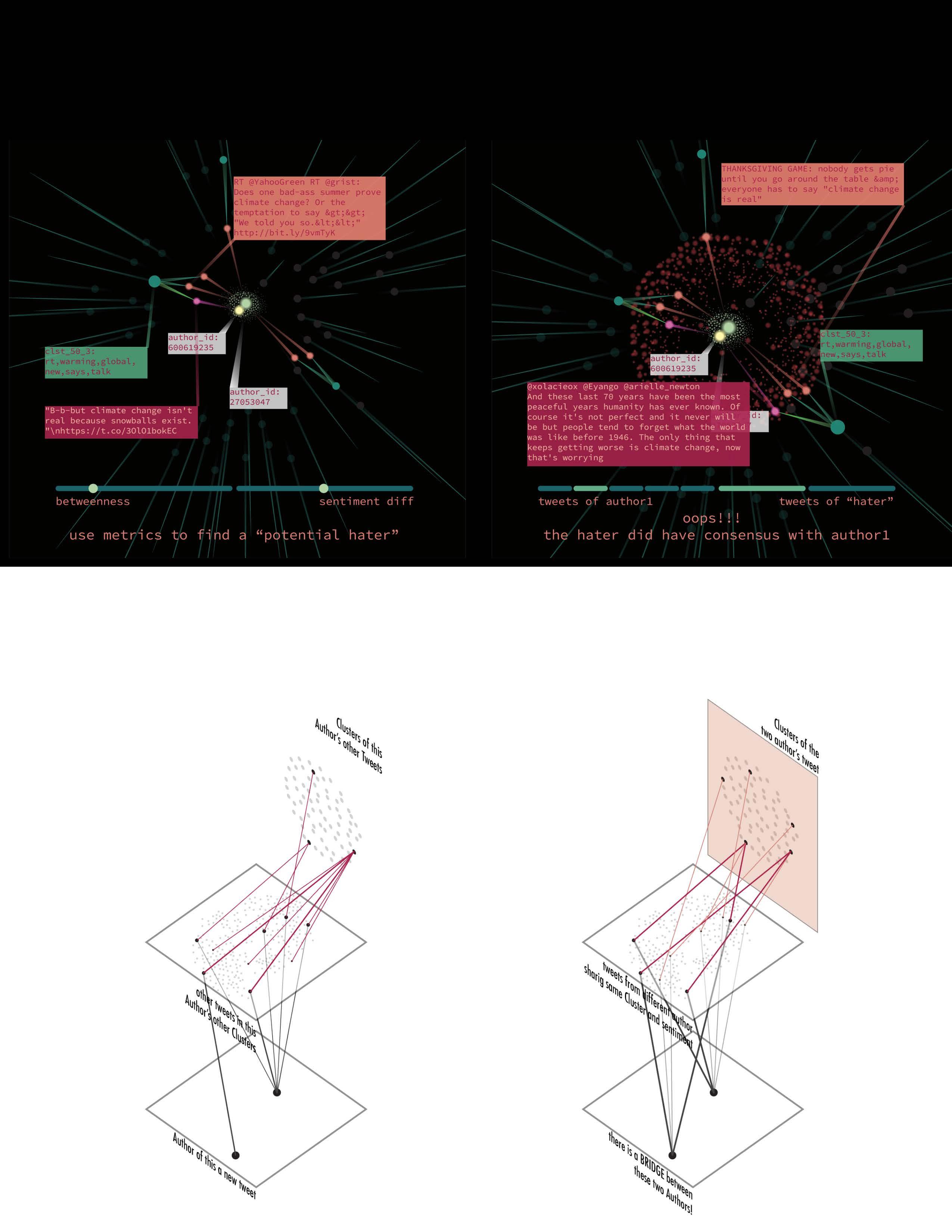
Opposite Author is not opposite in another cluster.

Under a cluster of other tweet from “author1”, another tweet is recommended by the graph, based on graph metrics like betweenness, tweet numbers, and tweets attribute sentiment. This new tweet from “potential hater” would have opposite sentiment with “author1”.

An ideal “potential hater” would have tweets with an overlap in clusters with that of “author1”, and under a same cluster tweets from both authors can be similar or opposite.

But other tweets from this “potential hater” could have similar sentiment with “author1”. Opposite authors in one cluster can have have consensus in another cluster.

Compare these two Authors across

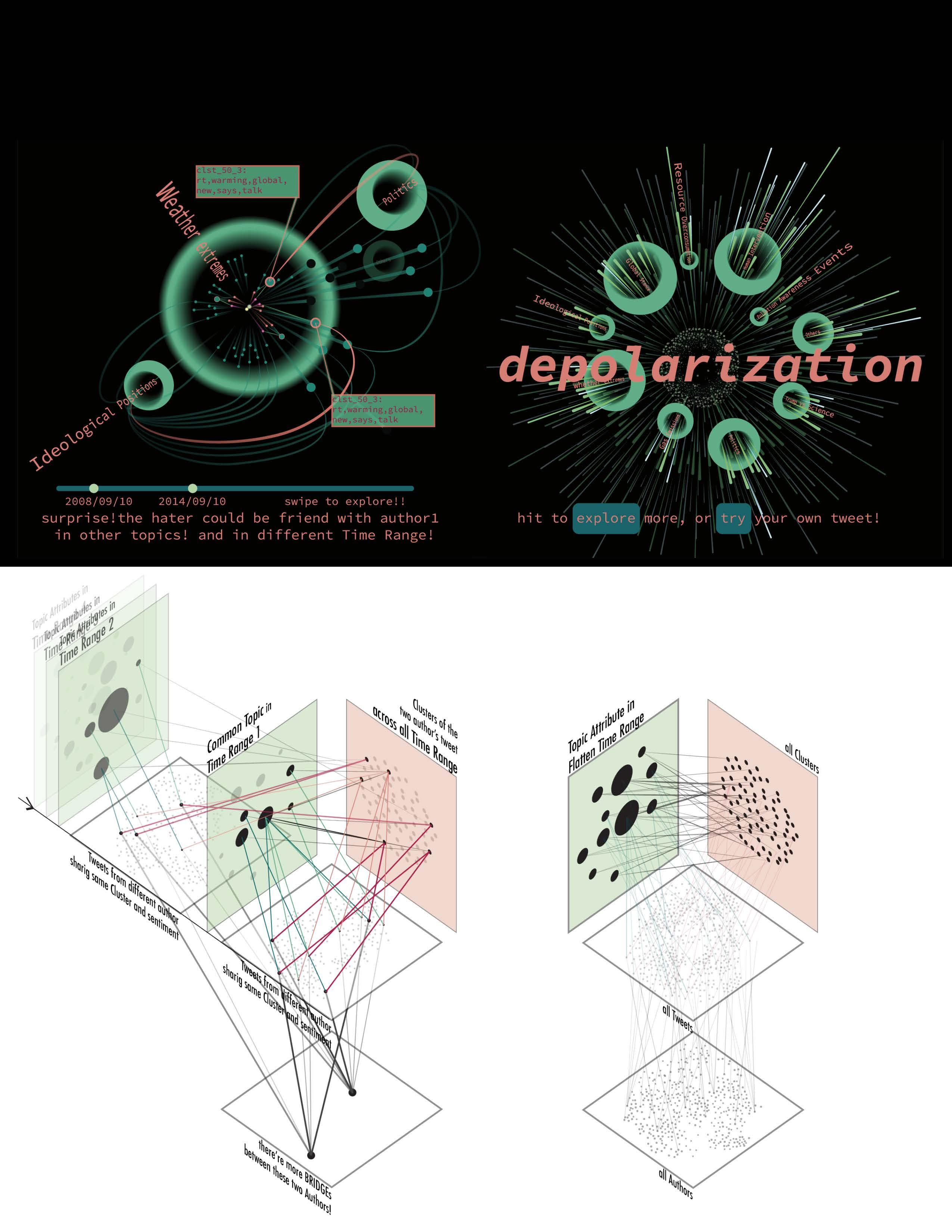
The comparation continues in more topics and more time ranges, the two authors did have more commons in other topics, some even across time range: “author1” in time range C would agree with “potential hater” in time range D.

After this initial exploration, user would have a more concrete image of polarization and echo chambers in social media. He/she is then encourage to continue the exploration with other discussion or try his/her own tweet, or bring this holistic graph browsing to other tweets he/she might be interested.

Experience: Browsing, Reflection, and Sharing

User Browsing

A New Paradigm for Social Media

1

2-3 C2:De-Polarization 5

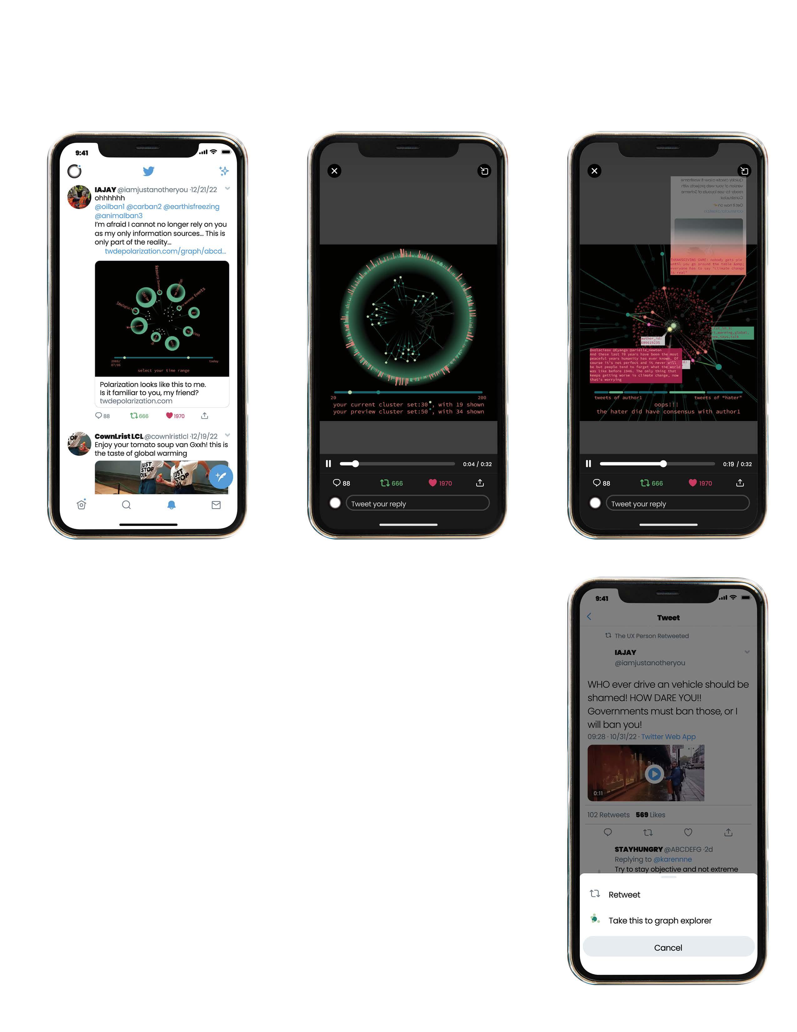
User finds someone sharing their thought with this tool in twitter and gets interested.

User see a short interactive demo of this graph, during which detailed tweet can pop up and allow user to get more concrete context. Content in this demo can be “adder to later”.

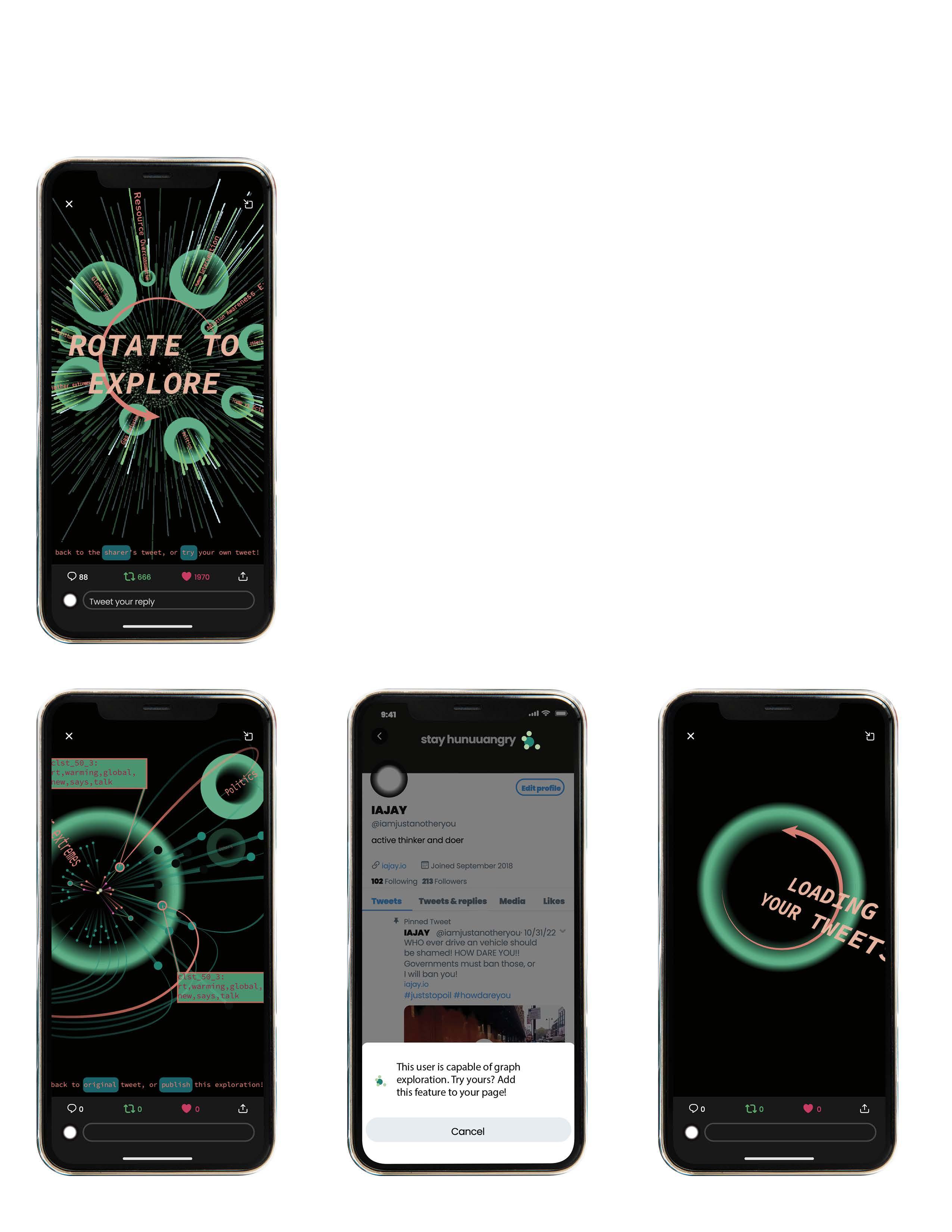
At the end of the demo, user is encouraged to continue explore the discussion, or with the user’s own tweets.

4 5

User explores content “adder to later” in more detail, here the user explore a tweet and its author’s other tweets.

User brings another tweets to the graph browsing tool, and plays with it.

7-8

User adds this function to his/her own page, starts loading his/her content in the graph, and start explores his latent datascape (or ideology).

a):

b):

c):

This graph view tool can be shared as an browsing journey that links tweets in a discussion, where other users can witness the change of stance and browse the detailed information in it a portal to explore other’s tweets in their context a introspective tool to navigate user’s own tweets and stance, throughout discussion topics and time range