Animal Farm—a complex artificial life 3D framework

Acta Univ. Sapientiae, Informatica 13, 1 (2021) 60–85

DOI: 10.2478/ausi-2021-0004

Attila KISS

J. Selye University Kom´arno, Slovakia email: kissae@ujs.sk

G´ab or PUSZTAI

ELTE E¨otv¨os Lor´and University Budapest, Hungary email: afbdpk@inf.elte.hu

Abstract. The development of computer-generated ecosystem simulations are becoming more common due to the greater computational capabilities of machines. Because natural ecosystems are very complex, simplifications are required for implementation. This simulation environment offer a global view of the system and generate a lot of data to process and analyse, which are difficult or impossible to do in nature. 3D simulations, besides of the scientific advantages in experiments, can be used for presentation, educational and entertainment purposes too. In our simulated framework (Animal Farm) we have implemented a few basic animal behaviors and mechanics to observe in 3D. All animals are controlled by an individual logic model, which determines the next action of the animal, based on their needs and surrounding environment.

1 Introduction

Within the concept of ecology, we treat an ecosystem as a small part of the whole living system. The ecosystem can scale in different sizes, from a local few species environment, to highly complex continent wide coexistence.

Computing Classification System 1998: J.4 Mathematics Sub ject Classification 2010: 68T20 Key words and phrases: artificial life, multi-agent systems, ecosystem, animal-simulation, extinction, sustainability, unity (engine), computer-generated, 3D-simulation, competingecosystem, ecosystem-model

60

Animal Farm 61

An ecosystem comprises the entirety of the living things (plants, animals) in a given territory, interacting with each other. Natural ecosystems are “balanced” structures. This means that through interactions between the individuals, ecosystems are constantly changing. With this changes, the system is constantly trying to stabilize and thus able to sustain for a long time. Every living creature has impact on the environment, like during their lifetime predators are hunting down smaller animals for food source to sustain themselves and grow their species population, while keeping prolific animal populations lower to reduce their noxiousness.

In the lifetime of an ecosystem there are many influencing factors that can change the whole image and future of the system. This factors can be abiotic (environmental impacts) like climate change, earthquakes and sea level rising; and biotic (living creatures and their interactions) like extinction of a species in the food web, new predator appearance from another neighbour ecosystem, human interference. This effects can make entire systems unstable, regardless of the complexity, size and thoroughly development by observations. Taking all aspects into account is impossible and the smallest undefined or random effects can alter the system in enormous ways.

Replicating small ecosystem environments with living beings is not an easy task. Animals’ behavior can become unpredictable in a few seconds, when they are reacting to outside effects (abiotic and biotic components as well) and every individual will react differently depending on their surrounding, characteristics and logic. This changes can force species to migrate or extinct, if their natural habitat changes rapidly and they can’t adopt fast enough.

Both fixed and random effects occur in the ecosystem. Fixed effects are well observed, monitored and known behaviors and characteristics of animals and the environment and most of the time simple to implement. Environmental effects can be remodelled in the system too, but hard to replicate realistically, because their strength and occurrence has to be set correctly, otherwise their impacts can be overwhelming. It is also hard to model animals’ logic and their behaviors (instincts) and how they react to different situations and occurring environmental and interaction effects. Their decisions is hard to determine based on purely outside effects or pure logic. Creating an ecosystem in a simulation is really difficult, because of this many unknown (indetermined or hard to monitor or remodel) factors. To imitate and simplify unknown influential factors, the most easy way to consider and determine them as random decisions and events as well. Without calculating these complex tasks and relying only on the values of the randomness, many alternatives are being created by running same simulations multiple times. While rerunning the same simula-

62 A. Kiss, G. Pusztai

tion and getting different result may sound odd, this way we can observe many alternatives of an evolvement of our ecosystem.

A 3D environment for a simulation can be useful to monitor different events and animals real time by graphical observation as well. It can show how the animals live, like when they eat or drink, and how they react to other species, like fleeing or hunting. It’s more an eye-catching experience to see the actual animals, rather than only reading the plain resulted statistics value of the populations. Also, while we can specify a lot of ways what and how to extract data form the simulations, sometimes it’s hard to determine what is important to extract from a situation. We can monitor what caused the animal’s death, say like it was killed by a predator, but this doesn’t determines if the animal wasn’t a suitable prey or just unlucky and couldn’t flee away from the predator due to a terrain (mountain or water) formation. And the opposite is true, when we say an animal died from like thirst, before it’s death, it could have been chased a long way by a predator, which would suggest to give the credit for the predator, but the system registered as a death of thirst, which in the plan statistics would imply a lack of water source on the terrain. Without a perfect register system, sometimes it is advised to check on the simulation’s 3D environment to observe interactions and events.

2 Related work

Scientists have been trying to analyse and model real ecosystems for a century. One of the earliest, and most well-known, ecological model is the predator-prey model of Alfred J. Lotka (1925) [17] and Vito Volterra (1926) [22] called “The Lotka–Volterra equations”. Volterra originally devised the model to explain fluctuations in fish and shark populations observed in the Adriatic Sea after the First World War. There are multiple alternatives to the Lotka-Volterra predator-prey model and its common prey dependent generalizations, like Richard G. Wiegert’s [23] simulation model or the Arditi-Ginzburg (ratio dependent) equations [2, 3] (it’s connection to Lotka-Volterra [21]) or a three species model, where two predator competing for the same prey by Reddy and Ramacharyulu [18].

In addition to mathematical models, there are also simulation models that can be used to model ecosystems, where the mathematical model is either too complex or impossible to compute. The difficulty of creating a model is, we need to include an enormous amount of factors and data (gathered or replicated), which could interact unpredictably with each other. In a simulated

Animal Farm 63

model, it is an always asked question, which attributes and effects should be included in the program. The best would be if we could replicate all the properties of the environment and the animals (this is what complicated mathematic models are trying to do). To reduce this complexity, simulated models typically simplify the systems they are representing, to limit the number of components. So simulation models are more widely utilized and more biologically reasonable, while analytic models are esteemed for their numerical tastefulness and elegance.

There are multiple other frameworks, which generate valuable ecosystem data, but most of them are using high abstraction in implementation (like only text-based or 2D environments and unrealistic creatures to study). In the ’90s, computer simulation programs were developed, modeled on the 1984’s programming game Core War [9], where two or more programs competed by switching turns to control virtual machines and get all the resources by terminating other programs. This kind of competition is similar to real-life ecosystems where the animals are rivals to each other. A simulation named Tierra [20] appeared to show this connection parallel, with the difference of evolvement, where the programs could alter themselves like an evolution approach to evolve. After a few years, another simulation called Avida [1] appeared with another addition, where “organisms” could have different execution speeds instead of a simple distributed turn switching. Many other improved and altered versions with modified rules appeared since then, like a modified model [4]. After this many variations appeared, the community decided to keep the basic approach, and an International Core War Society (ICWS) was established for the maintenance of Core War standards and running the tournaments.

Meanwhile, computer graphics improved and finally allowed to create graphic representations of the simulations. With graphics, we became closer to replicate and observe real ecosystem environments instead of just creating simulations with complex calculations showing numbers on the screens like mathematical ecosystem models. Some simulations take a 2D abstractions to simplify their model and save computer resources like Bubbleworld.Evo [19]. Bubbleworld.Evo is a multi-agent simulation where hundreds of prey (bubbles) are trying to avoid predators (triangles) to survive. The agents determined by size, energy, speed, and in their life cycle, when they reach a dedicated size or energy, they reproduce into multiple offsprings, starting their live cycles again from the start.

Creating simulations where the animals have complex logic has many cons and pros. If they are very complex, their behaviors will be hard to define

64 A. Kiss, G. Pusztai

and control, and also calculating this for every individual requires significant computer resources. A 3D simulation called PolyWorld [24] created trapezoid agents to search for food and mate. They needed to keep their whole population only in the hundreds to be able to run. With lower population numbers, it is hard to create any solid ecological statements.

Another 3D simulation is Framsticks [15, 10, 14, 11, 12, 13], but here, they took a very unusual approach to the animal models and evolution mechanics. The creatures contain mechanical structures (“bodies”) and control systems (“brains”), which results in very unusual appearance, like stick segments with joints. Their complicated system requires a ton of physics calculations like collisions with other creatures and the environment, gravity, and mechatronics forces (friction, elastic reaction). However, if we have enough computation power, we can run different enormous, physically accurate experiments, including evolution optimizations, co-evolution, and spontaneous evolutions from gene pools.

3 Simulation environment

While scientists like to analyse data from simulations, to catch other (like younger) audiences’ interest, the simulation has to be just as engaging as informative. We named our simulation framework to “Animal Farm” after George Orwell’s novella as an indication of the animals’ logic model, where they can behave unexpectedly (and “rebel against us” as in the novella’s story).

To make our immersive 3D graphical simulation we used Unity (engine). Unity [27] is a cross-platform game engine, developed by Unity Technologies. The editor is supported on Windows, Linux, and macOS, but the engine can build applications for more than 25 different platforms. Unity integrates multiple custom rendering options with an incredible physics engine and with Mono, the open-source implementation of Microsoft’s .NET libraries, with we can write scripts in the ob ject-oriented programming language C# to create and control the running simulation. Unity is well documented and constantly upgraded and supported with many official and unofficial tutorials on the internet.

In the past, many graphical engines were used to create 3D environments, but the most popular was the Unreal engine. After the launch of Unity in 2005, many developers and pro jects like “Search and Rescue Game Environment” [5] moved to this new platform. The editor is a well-designed environment with a lot of features and options like drag-n-drop features and built-in windows

Animal Farm 65

and also custom windows, which can be easily created by ourselves to use in our pro ject to make the work easier.

In the past, Unity had only paid options, and Unity Indie was the cheapest with limited features, but after 2009, they discontinued the Indie version and released a free Unity version with very few feature locks. Unity’s policy is that Unity (Personal) is free to creators with revenue or funding (raised or selffunded) below USD 100K in one year, meaning after 2009, a large number of students, hobbyists, and Indie developer had the opportunity the start pro jects with Unity for free. To unlock all the features and functionalities, a Plus or Pro license is required, but year after year, many paid features have been moved into the free version, which makes Unity an amazing platform to use for smaller, Indie development and for scientific demonstration purposes. You can learn more about Unity’s history in [8].

4 Our work

In our pro ject, we are using our developed multi-agent predator-prey simulation model to create an isolated 3D environment with a few example species. From the simulations, we collect data to analyse and set up certain hypotheses. Our animals are not simply separated into 2 distinct groups (predators and prey), we created a model, which supports food chain approaches too. A medium-sized animal can be the predator of a smaller animal, but an even bigger animal could consider this medium-sized animal as prey.

In our simulation, the animals can move intelligently on a terrain with Unity’s AI system, which provides a navigation mesh, by scanning the terrain and creates a walkable mesh. On this mesh, we can set a position as a destination point for the animal. The AI system will calculate the shortest path to our destination with obstacle avoidance (like hills, trees, lakes).

To provide land for our animals, we created two separate modes (called Sample and Custom scene). The Sample scene contains a premade, static terrain created with Unity’s Terrain Editor and 3 lakes, many trees, and at the edges of the map a range of mountains to keep the animals on the map. The Custom scene is for self-made maps, where we can import terrain data using heightmaps (more in the designated section) and modify it in some aspects, then start the simulation on your newly created map.

Both scenes have a ‘Console Prompt’ feature (by pressing the TAB key) where, with specific commands, we can interact with the running simulation like, spawn and reset animals, manipulate time, get statistics of the animal.

66 A. Kiss, G. Pusztai

Two camera modes are possible, the default is to fly around inside the simulation (WASD keys) to inspect the animals, and a follow mode to automatically follow an animal (by left-clicking on the animal, which you want to follow).

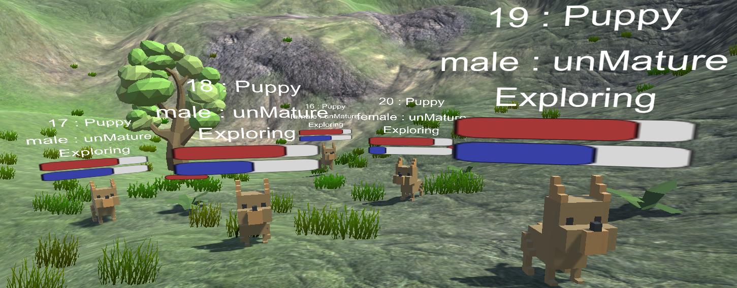
Above each animal, you can see primary information of the animal’s thirst, hunger levels, current logical and mating states, the animal’s age, age stage, and the pack’s name, which the animal belongs to.

To create some of the graphical and technical parts, we used free assets from the official Unity asset website [28]. The animal models are from 2 packages, the “Voxel Animals Pack” from “Total Game Assets” [33] and “5 animated Voxel animals” from “VoxelGuy” [29]. Our vegetation models are from the “Low Poly Nature – FREE Vegetation” from “Elcanetay” [31] and the tree models “Free Trees” from “Ada King” [30]. We have used a file browser implementation for importing heightmap images into our custom map generation “Runtime File Browser” by “S¨uleyman Yasir Kula” [32].

5 Featured mechanics and logical phases

5.1 Exploring mechanic:

This is the default phase mechanic, if no other mechanics’ criteria are fulfilled (e.g., the animal can’t see any water in view range, when thirsty), the animal will explore the area, until a needed resource or an enemy is found. If the pack mechanic is turned on, the animals will explore together, following the pack leader.

Figure 1: Exploring mechanic

Animal Farm 67

5.2 Drinking mechanic:

If the animal’s thirst level is below a set threshold and a designated water source found within view range, the animal goes to the source and starts to refill its thirst (lower, blue bar) meter.

Figure 2: Drinking mechanic

5.3 Hunting mechanic:

If the animal is a predator and the animal’s hunger level is below its threshold and a designated food source found within view range, the animal starts to hunt the prey by following it and if reaches close proximity, kills the prey. The prey’s body becomes a corpse and the predators can consume it.

Figure 3: Hunting mechanic

5.4 Eating mechanic:

If the animal is a vegetarian or the hunting mechanic is completed, the animal goes to the food source (the hunted animal or the plant) and starts consuming it. The feeding is represented by filling up the hunger (upper, red bar) meter, and the source’s meter (single, red bar) drains. Additionally, the corpse’s

68 A. Kiss, G. Pusztai

source fades overtime, representing flesh decomposition and the vegetation’s source is increases overtime as the plant’s natural regeneration ability. When the source is completely depleted, it disappears from the simulation.

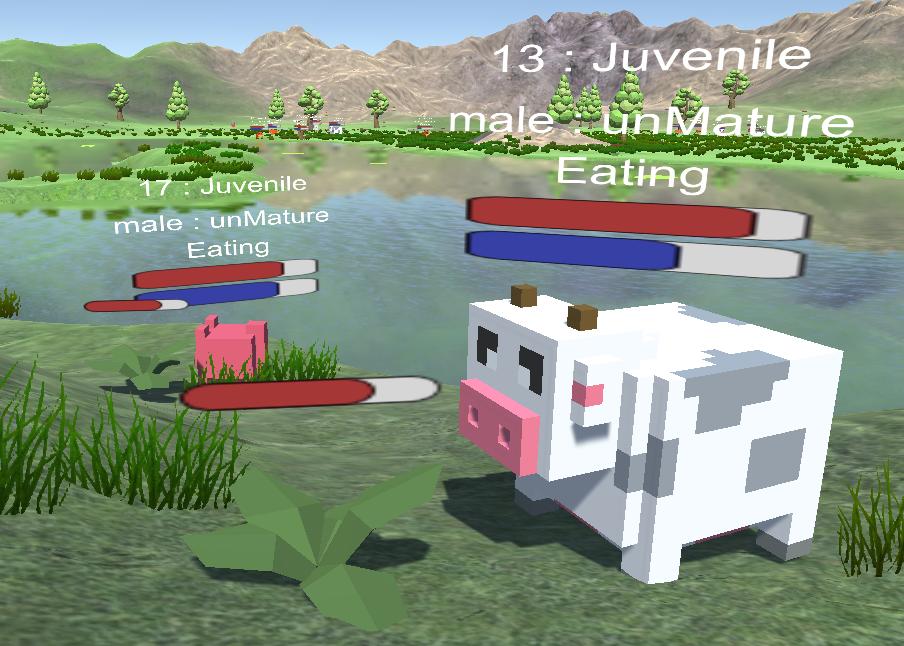
(a) Predator eating

(b) Vegetarian eating Figure 4: Eating mechanic

5.5 Fleeing mechanic:

If the animal senses a hostile animal within the view range, a fleeing movement overrides any other mechanics and the animal starts to run in the opposite direction, trying to escape from the predator. If the prey loses the predator, the natural logical cycle is restored and continued.

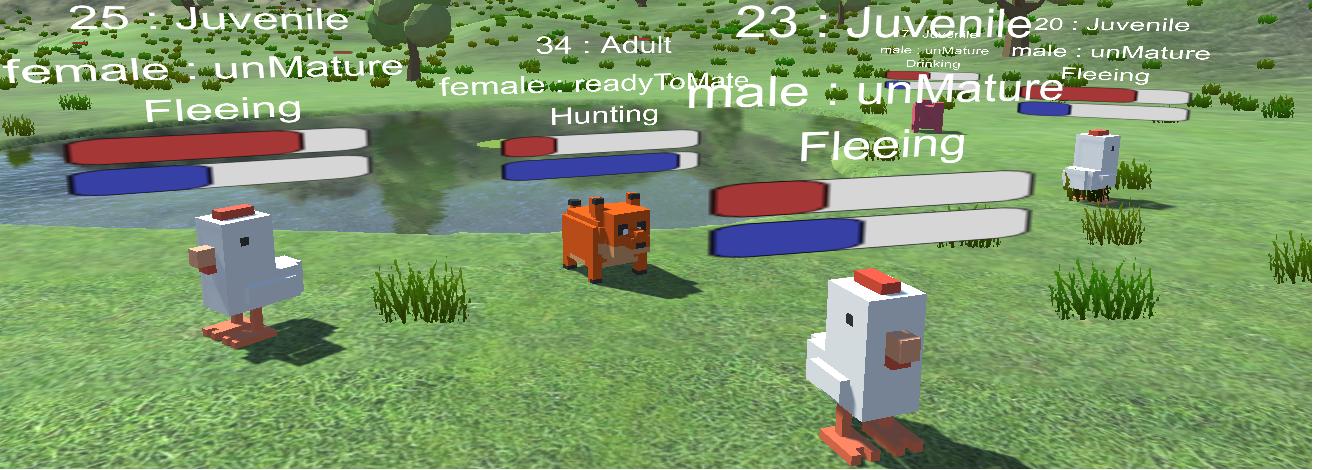
Figure 5: Fleeing mechanic

5.6 Mating mechanic:

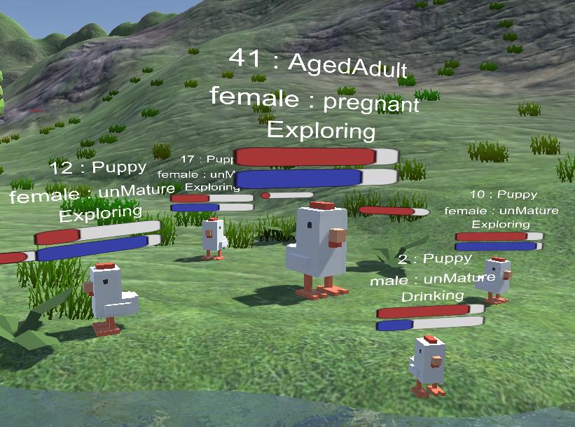
Within the view range, if the animal finds a right (gender, mating and age status requirements are fulfilled) partner, a mating request is sent by the male to the female, and if it is accepted by the female, they will start the mating

Animal Farm 69

process, which will result in the female becoming pregnant. After the pregnancy time ends, new children are born (depending on the species childbirth capability).

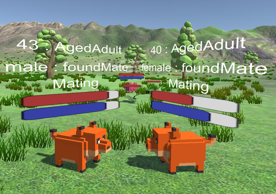
(a) Finding a partner

(b) Creating new life Figure 6: Mating mechanic

5.7 Pack mechanic:

The animals can form packs with others from their own race. During the simulation, multiple packs can be formed for each race (in this simulation animals will always try to form bigger packs until a set maximum threshold number is reached), an individual can request a join (even change, which pack they belong) to an other pack, which could be accepted or rejected. Every pack has a leader, whose movement will be considered during an individual’s exploring logic phase. This results in a group of animals, which moves and sticks together. This mechanic has many positive (e.g., easier to find mating partners) and negative (e.g., predators will find and catch preys easier) qualities. These assets have been analysed with statistics at the end of the article.

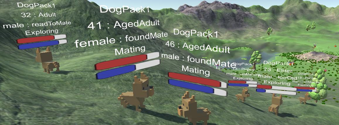
Figure 7: Pack mechanic

70 A. Kiss, G. Pusztai

6 Adjustable parameters in the simulations

To modify any animal parameters, we have to alter their species’ attributes. There are many attributes, which control the behaviors of the animals and they can be set for all species separately. First, we have to set a race type, so the animal knows, which animals are in the same race, to consider them as allies. Addition relations are the list of enemies, where the animals who belong here will trigger the fleeing mechanic, and the list of foods, which determines the animal’s feeding type and which sources (animal or vegetation) to look for to trigger the hunting and eating mechanics.

There are some parameters, which change as the animal grows. These variables can be set to animals depending on their age stages. Animals are categorised into age stages based on their current age. Our pre-determined age stages are Puppy, Juvenile, Young, Adult, Aged, and Elder. Inside every age stage, there are 4 primary variables: view distance, walking speed, hunger modifier, thirst modifier. View distance means, how far the animal can see, and from this information, the animals will determine what to do. The walking speed means how fast the animal can move on the terrain. The hunger and thirst modifiers alter the basic life requirements (metabolism), where the animals always lose hunger and thirst, while the time passes. With this, we can determine characteristics for different ages, like older animals’ metabolism slows down, so their hunger and thirst bars will decrease slower than an Adult’s from the same species, but their view distance and walking speed decrease as well.

The mating mechanics is determined by age stages too, where the Puppy and Elder can’t reproduce, meaning they will be in a not sexually active status, but other stages can. Males and females have unique attributes here, females have pregnancy duration and max childbirth capacity, and males have spermatogenesis duration, which means the length of a state, when the male sexually inactive.

With the pack forming ability, we can set which species use this mechanics. If they are capable to form packs, the species will start to create groups and move together, if not, every animal stay an individual from others (except in the mating mechanic) and explore the map separately.

7 Custom map generation

In this simulation environment, we can choose between 2 maps to run our simulation. The first is a sample static map, which was created by hand to test the

Animal Farm 71

animals and illustrate a beautiful landscape, while our simulation is running, but due to its static nature of the map rerunning with the same properties multiple times, will end in slightly similar results, because of the landscape’s image (lakes’ and hills’ position). According to solve this problem, we created a tool to import custom maps into the simulations, using heightmaps. A heightmap [6] is a black-white image file containing data from a landscape, where the pixel positions are representing the 2D surface coordinates and the pixel’s grey shade will represent the height in a 0-1 scale. This allows us to convert an image file into a 3D mesh surface (terrain map), which our animals can walk on. Heightmaps include water on their representation (usually the darkest areas) but we can’t be sure if that area is water or land with sea level 0, or even below sea level. In our generator section, we provided some tools to scale, increase, set a maximum height and set water level after the image is imported to modify the terrain as we wish, and see the modifications in real-time inside the environment. After we are satisfied with the map, pressing the start button will calculate any furthermore necessary technical details, and start the simulation like the sample scene, except this time with our custom-made map.

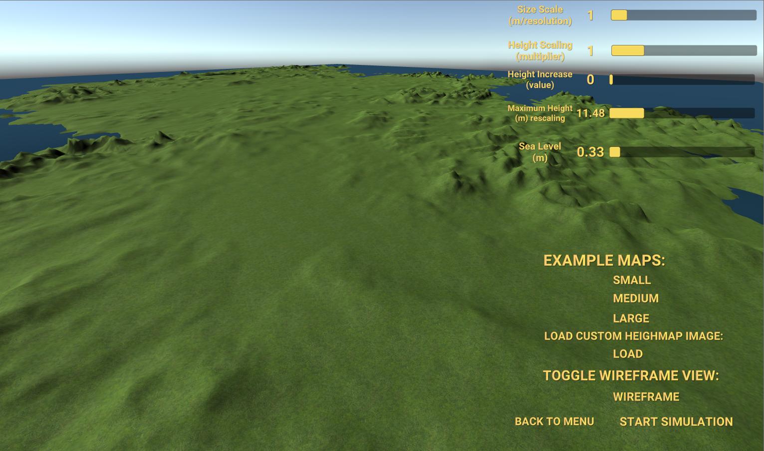
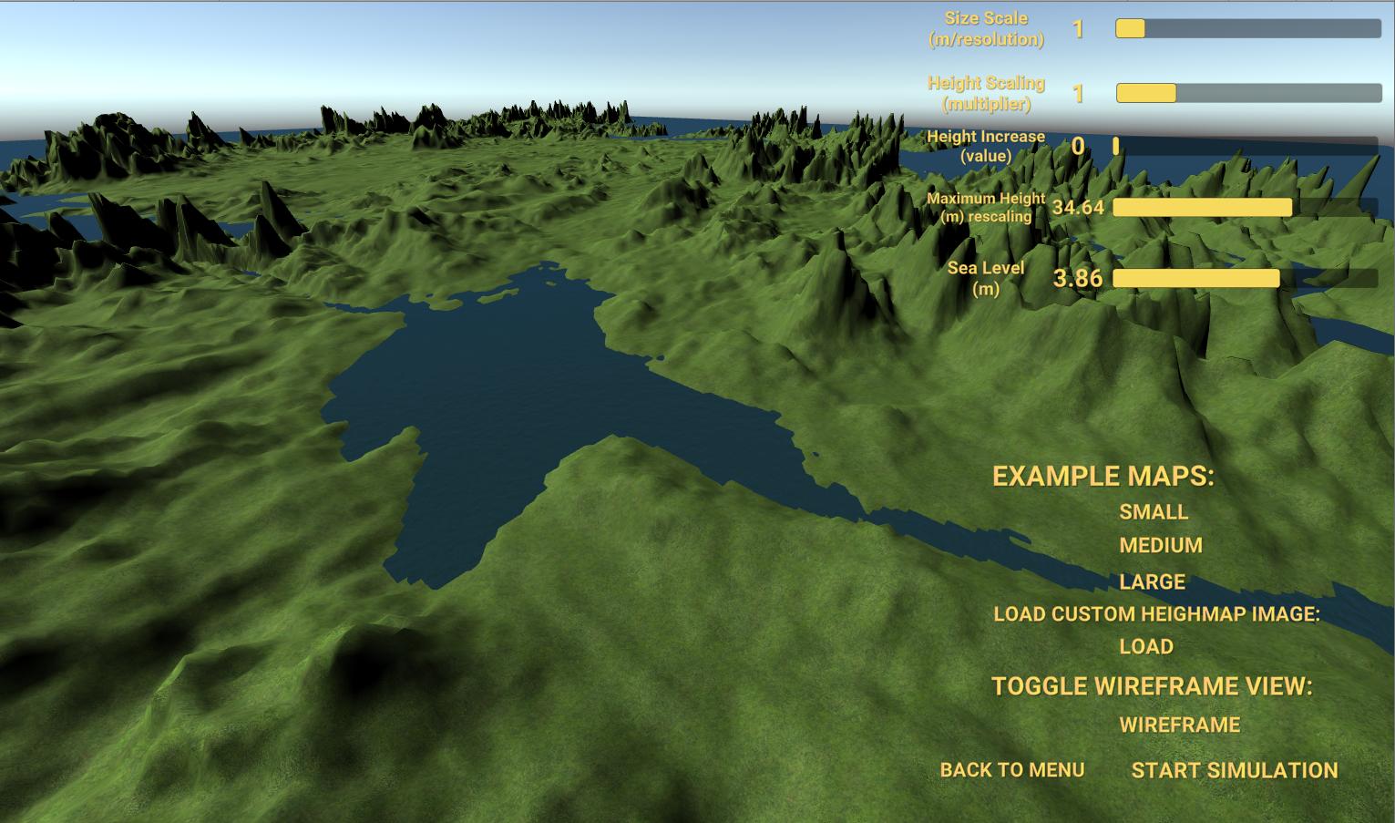
(a) Plain terrain with low sea level (b) High mountains with higher sea level

Figure 8: One of the 3 example maps provided inside the program, the same heightmap was used in both pictures, only the maximum height and the sea level was modified at runtime with the right-upper modifier sliders.

8 Heightmaps

As described in the previous section, we need an image to start a custom simulation. There are various different methods to acquire images like searching online, using any search engine, which is a great way to gather varied types and shapes to run an experiment. If we want a specific location’s

72 A. Kiss, G. Pusztai

heightmap on Earth we can search for it by name or we can use “https: //terrain.party/” website to create our own snapshot of a part of the Earth. Or, if we would like to run our simulation on many different (unreal) terrains we can use a noise heightmap generater like “http://kitfox.com/projects/ perlinNoiseMaker/” to generate a random terrain to import into our environment.

Inside the map generator, we can modify a heightmap image with 5 different attributes. The “Size scale” will scale the whole image to a bigger terrain. “Height scaling” multiplies every positive height value. “Height increase” adds this fix value to every positive height value. “Maximum height” sets and translates the original heightmap’s 0-1 value into the simulation’s value system, meaning if a point is 1 (the most white color) on the heightmap, inside the simulation, it will be 11.48 (example value from [Figure 9b]) units tall. And the final attribute sets the “Sea level” to a designated value.

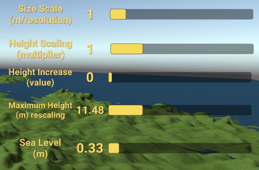
(a) Heightmap of the example [Figure 8] (b) Changeable heightmap variables

Figure 9: Heightmaps

9 Demonstration of the platform

For demonstration purposes, we have created 6 prototype animals with different properties and 1 plant with a fixed 9-second reproduction rate and random spawn positions. The animals’ names are only for demonstration purposes, we named them randomly (considering some attributes as animal characteristics to strive for realistic representations of the real world animals). We named our only plant type “Grain”. We planned to create multiple types of vegetation, but decided to keep only one for this demonstration, because there are only 3 vegetarian types, and we didn’t want to complicate the experiments and decided to set them as to eat the same type of vegetation.

Animal Farm 73

Parameters Chicken Pig Cow Dog Fox Lion Avarage lifetime 375 700 800 650 550 700 Most childbirth 3 3 1 1 2 1 Pregnancy dur. 55 70 80 65 65 70 Spermatogenesis 50 30 30 30 30 30 Food Grain Grain Grain Chicken Chicken,Pig All Enemy Dog,Fox,Lion Dog,Fox,Lion Dog,Fox,Lion Lion Lion,Dog None

Viewrange Chicken Pig Cow Dog Fox Lion Puppy 20 22 22 23 26 23 Juvenile 22 24 24 25 28 25 Young 23 24 26 27 30 27 Adult 25 25 28 29 32 29 Aged 22 24 24 25 28 25 Elder 18 22 21 21 24 21 Walkingspeed Chicken Pig Cow Dog Fox Lion Puppy 3.3 3.2 3.2 3.55 3.65 3.5 Juvenile 3.6 3.6 3.4 3.85 3.85 3.65 Young 4.1 3.9 3.6 4.05 4.15 3.85 Adult 4.3 4.1 4 4.2 4.25 4.1 Aged 3.7 3.6 3.4 3.7 3.85 3.55 Elder 3.2 3.1 2.9 3.2 3.35 3.3

Thirst/Hunger Chicken Pig Cow Dog Fox Lion Puppy 1.3 1.1 1 1.1 15 1.1 Juvenile 1.55 1.35 1.35 1.3 1.35 1.22 Young 1.65 1.5 1.5 1.4 1.45 1.3 Adult 1.55 1.4 1.35 1.3 1.35 1.2 Aged 1.25 1.3 1.1 1.1 1.15 1.1 Elder 1 0.9 0.8 0.7 0.7 0.7 AgeStage bound. Chicken Pig Cow Dog Fox Lion Puppy 37.5 105 120 97.5 82.5 105 Juvenile 75 154 176 143 121 154 Young 112.5 231 264 214.5 181.5 231 Adult 187.5 350 400 325 275 350 Aged 281.25 525 600 487.5 412.5 525 Elder 375 700 800 650 550 700

9.1 Sample results

We ran simulations with the same parameters and heightmap multiple times, and from the generated data we created summary graphs for each simulation. Here, we represent 5 unique situations to analyse, which were different form the ma jor of the results.

For these simulations, we created a custom made map with balanced landwater ratio and distribution in our opinion. We placed 9 circle shaped lakes on a big square land, where the animals had plenty of space to go around and between the lakes. This way the combined water surface area was around 35-40% of the map. The water itself shaped multiple natural obstacles for the animals, so we didn’t add any mountains to this terrain, to give the preys plenty of opportunities to flee in multiple directions without trapping themselves.

Our simulations start with spawning the designated number of animals (24 chicken, 24 cow, 24 pig, 18 dog, 18 fox and 12 lion) on the map with random positions. The spawned animals start as newborns on random positions, with their properties reduced to their current age stage of their species’ characteristics. Because, the predators are already capable of hunting when they young, sometimes they spawn close to the preys and start to chase them in everywhere on the land, which creates a chaotic start of every simulation. From

74 A. Kiss, G. Pusztai

this chaos, unfortunately only a few species come out alive, usually 1-2 vegetarian and a predator type. Later the survived animals’ numbers normalize and they start to create different symbiosis variations for a short time. Also, because the terrain is an isolated land from other ecosystems, there are no outside effects to our ecosystem, and if a species extinct there will be no more of them to observe in the simulation. We tried to balance the species capabilities (demonstration attributes), but this only resulted in a random selection of which animals survive the start chaos.

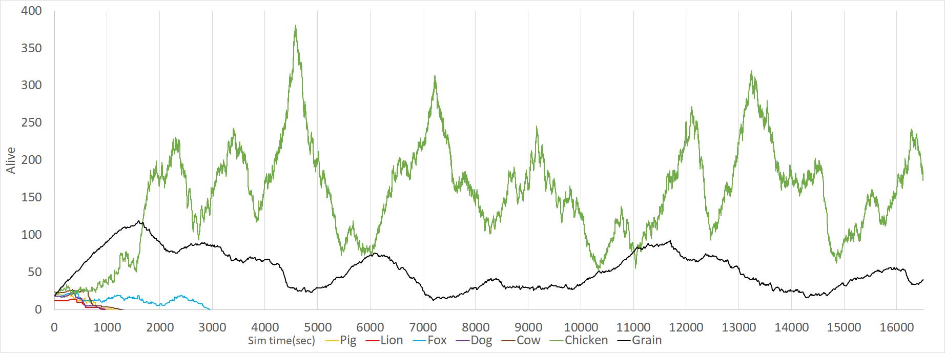
Figure 10: Symbiosis between vegetarian animals and the vegetation

[Figure 10] shows a unique case where only 1 vegetarian animal (chicken) survived in the long run of the simulation. We can observe a very balanced symbiosis between our chicken and grain species with a natural both-sided waving population increase and decrease. The chicken fluctuates in waves with the vegetation due to their rapid reproduction rate, when their numbers reach a high value they start to eat more vegetation than the vegetation’s reproduction rate and the vegetation starts to decrease, which results a low food supply for the high number of chickens and they start to starve to death, lowering the chicken’s number, letting the vegetation to replenish and at a point, it will be able to sustain the lower chicken population again. Without any predator the chickens’ only danger is their own gluttony, meaning if the vegetation hits a very low value, maybe there won’t be enough time for the vegetation to recover before the whole chicken population starve to death.

Animal Farm 75

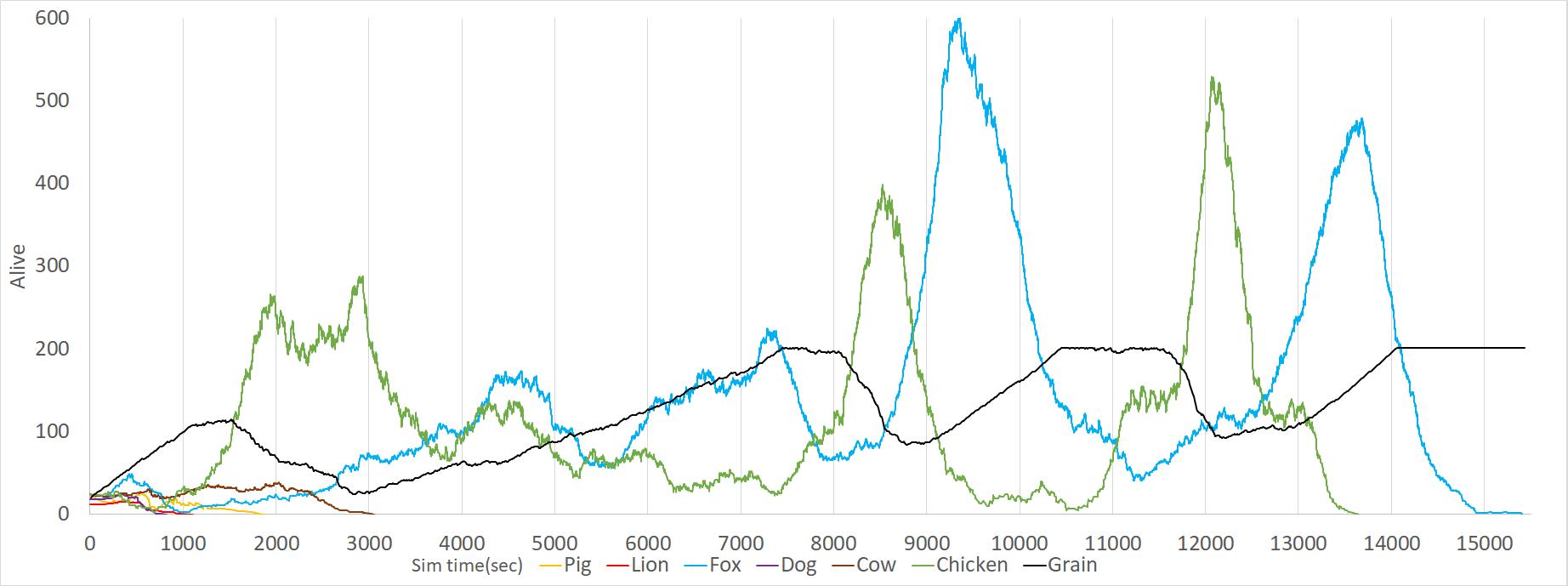
Figure 11: Symbiosis between 3 species

In this simulation [Figure 11] we can observe a more complex symbiosis between the chicken, fox, and grain. Chickens multiply rapidly, capable of a fast recovery in numbers, resulting in a grain decrease first and a fox increase secondly. The foxes overcome of the chickens’ number and will decrease them significantly. If the low chicken population can survive for a brief time, the foxes number will decrease due to the food shortage, resulting in a fox population shrink and the cycle can restart. Unfortunately, this simulation ended, because after the second huge fox population wave, the chickens couldn’t sustain themselves against the foxes and died out.

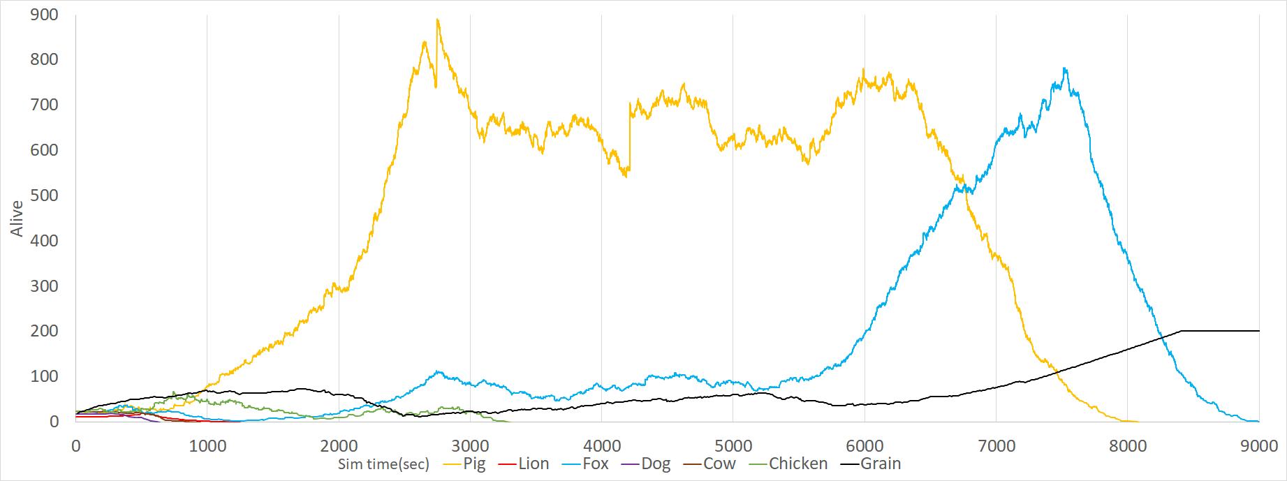
Figure 12: Pigs have eaten all the food from the chickens

Here [Figure 12] pigs overpopulated the map. Pigs have a slower reproduction rate, but because of the early low population of the foxes and the other predators’ extinctions, pigs by chance could overcome of the chicken popula-

76 A. Kiss, G. Pusztai

tion, which extincted because of the food shortage and their low population number soon reached zero. The chickens couldn’t reproduce enough, because the pregnancy and childbirth infer an extra hunger modifier, which if not enough food is available, could be fatal for the population. Foxes could barely survive, but at the early stages, pigs and chickens provided enough to reach a safe number, and after the chicken’s extinction the foxes started to eat the pigs and their population started to grow rapidly since they didn’t have any enemy. When the foxes population grow higher, the pigs couldn’t keep up with the hunt and their numbers started to go down, which resulted in their and after a short time the foxes extinction.

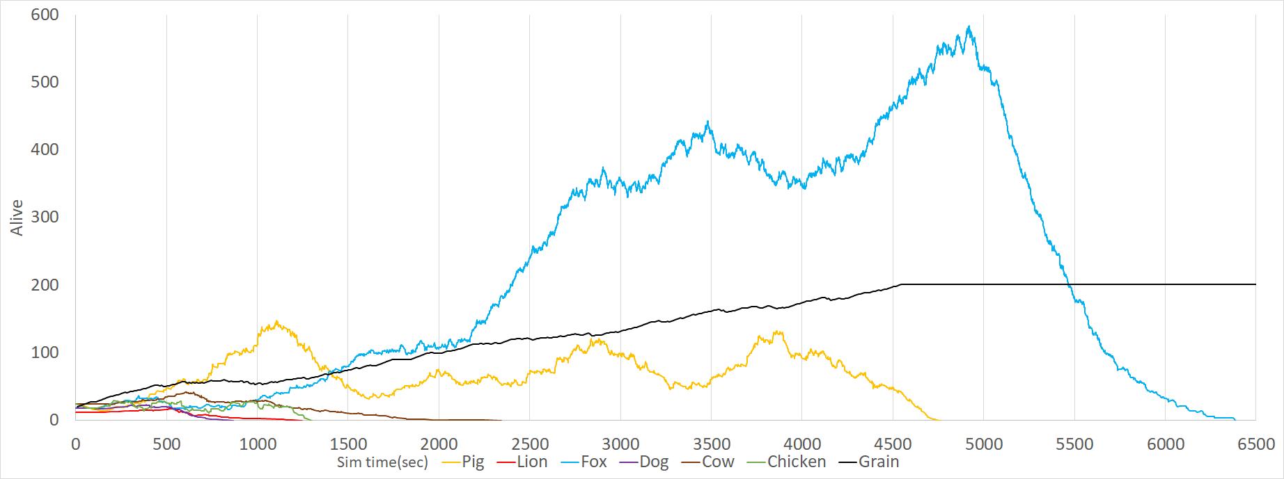
Figure 13: Unsustainable symbiosis

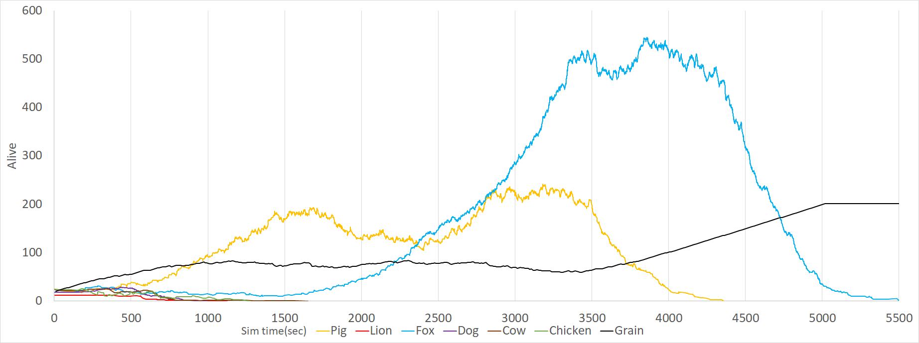
Figure 14: Unsustainable symbiosis 2

[Figure 13] and [Figure 14] is a more common result, rather than [Figure 12], because the pigs are not as prolific as the chickens and with an even slower

Animal Farm 77

start as before, they extincted even faster, because the foxes hunted them at the same rate, but due to the low population, the same scenario happened, just earlier. This means, that the chickens and foxes could perform better in a predator-prey symbiosis, rather than the pigs and foxes. Pigs have an advantage against the chickens with a longer lifetime attribute, but have the disadvantage in their pregnancy duration. If the predators are hunting the preys rapidly and the prey dies before reaching an older age, the extended lifetime has no real advantage, but the faster reproduction rate could mean the survival of the prey population, which the preys in the real world also use for survival.

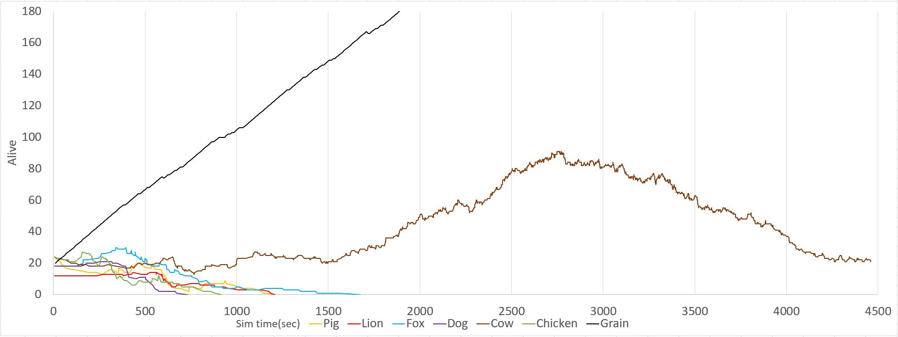
Figure 15: Bigger size is not always an advantage

In our last demonstration, the cows survived the chaos alone, like in our first demonstration [Figure 10] with the chickens and the vegetation. In the cows’ characteristics we have given them a much lower reproduction and movement skills on purpose. Their only two advantage is in their size (out of our predators, only the lions can harm the cows) and their expanded lifetime. As the only survivors, without any enemy and plenty of food, they managed to survive, but unlike the chickens their numbers didn’t fluctuate as much, keeping a low population despite the food abundance, due to their low reproduction rate their population kept a low value. Without predators or environmental effect this can be an acceptable solution, but if the lions were present or any catastrophe (e.g., environmental event or biological disease) occurs, while they keep a low population, they wouldn’t survive for long and extinct.

78 A. Kiss, G. Pusztai

9.2 The pack forming ability and the advantages of the mechanic

To demonstrate the pack forming ability usefulness, we ran multiple simulations with the same animals (types and properties, same animal starting numbers), on the same terrain with random starting points, the only thing we changed is the pack forming ability for all or none of the animals. Without a cohesion force, the animals make their decisions fully separately from each other (ignoring each other, except in the mating process) and with the packing mechanism the pack’s members always try to stay and move together.

We observed our prey animals (Chicken, Cow, Pig) more closely, because they had a more a more notable change in their populations than the preys’ .

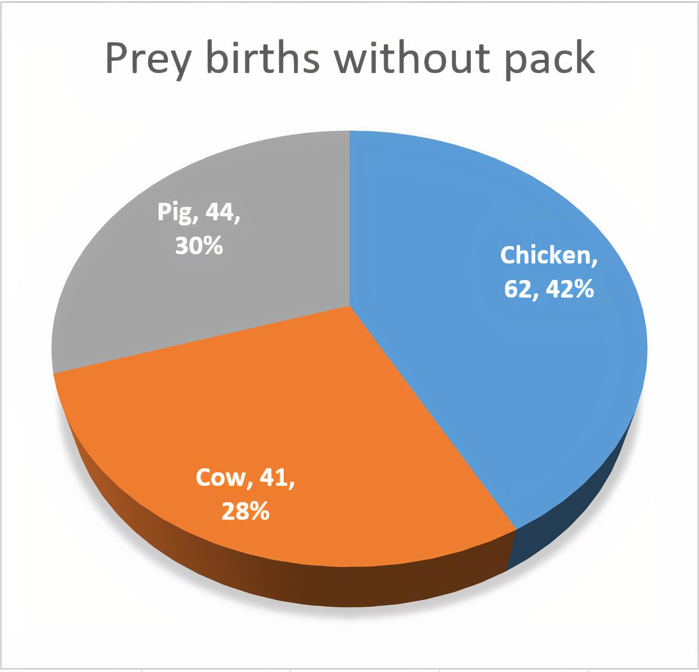
Hypothesis 1 (H1): Forming a pack could benefit in the mating process, because the animals are close together and they don’t need to search long for a mate to reproduce which wil l greatly increase the population.

The simulations support this assumption. The prey animals have a default faster reproduction rate than the predators, furthermore the mating process is accelerated rapidly due to the close distance between the species, because the animal doesn’t have to spend a lot of time to find a suitable mate.

(a) Without pack

(b) With pack Figure 16: Prey animals’ birth numbers.

The difference between these 3 animals is we have given them different maximal child births at labor (pig 4, chicken 3, cow 1).

Hypothesis 2 (H2): Forming a pack also could improve their lifetime or help in their species survival.

The simulations support this assumption as well,

Animal Farm 79

1. With the growing population (shown in Hypothesis 1) the predators have a lot more food source to ease their hunger, which extends the predator’s lifetime.

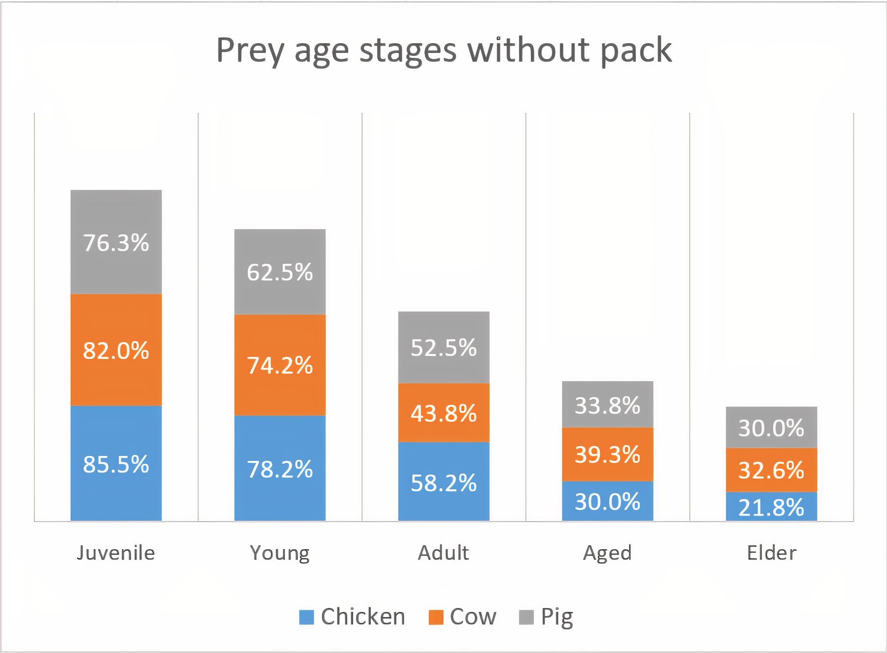
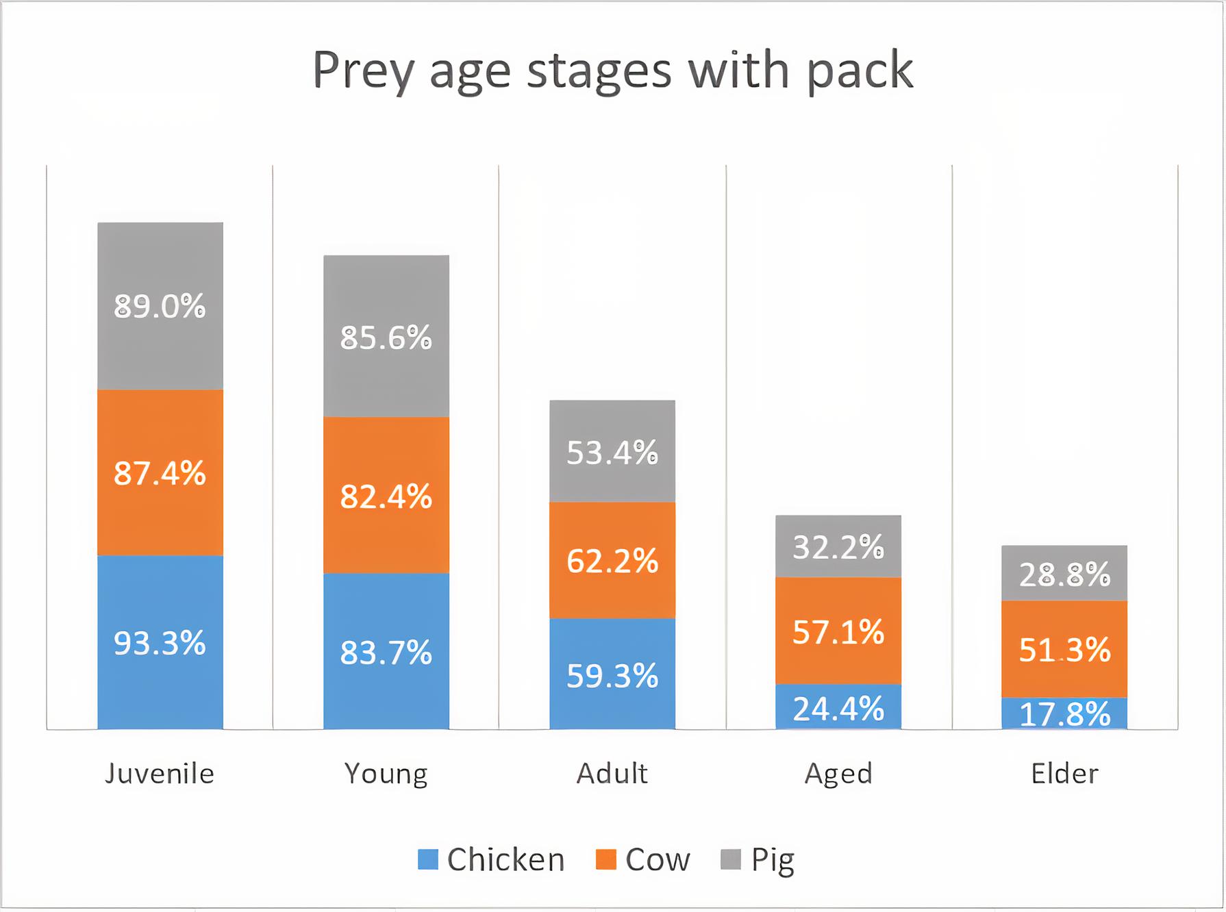
2. In a pack, animals with different ages are staying close together. When a predator attacks, it will choose the closest prey to catch. The younger ones, because they have more speed, they can flee more quicker than the older members of the pack. The predator will likely change it’s hunting target to them, because they are easier to catch. After the successful hunt (and the tragical death of an elder) the predator becomes satiated by consuming it’s prey and leaves the pack alone for a while. With the survival of the younger animals, the pack has more repopulation ability, which extends the pack’s and also their species’ survival.

(a) Without pack

(b) With pack Figure 17: Prey animals’ reached age stages

Here we can see the dispersion of the reached age groups. This means, if an animal dies in it’s current (e.g., Adult stage), it will be counted in the previous (Juvenile, Young) and current (Adult) groups, but not in the following (Aged and Elder). The percentages show how much of the population has reached that designated group, for example in [Figure 17a], 85.5% at the Juvenile column’s Chicken section means that 14.5% died early at the age of Puppy. The pack mechanic had a greater impact on the younger groups, but all groups had an increase in their combined (value of considering the 3 animals together) number.

Hypothesis 3 (H3): Sticking together has it’s danger, when predators attack they can surround more prey at once or in a shorter time.

In our simulation, every animal was set as scavengers carnivores, whom consume corpses. With this presumption this hypothesis considered as false.

80 A. Kiss, G. Pusztai

1. If the predators attack in a large group, they can surround an area, but they will likely target one or few of the prey at once (shown in

Hypothesis 2) and most likely catch older preys, additionally, when a predator catches a prey, other predators, if they are close, they can leave their hunting target to escape and join in the corpse consumption, this way no leftover from the corpse will go to waste (predators hunger will be more efficiently satisfies) and the hunt for the pack’s other members will only continue if the predators are still hungry.

2. If a member of the pack dies in natural causes, like due to thirst, hunger or age, the predators who followed the pack, but didn’t attack yet, can find the recently deceased animal’s corpse easier and consume it, if they are scavenger carnivores. Without the pack function, the deceased animal can die in an abandoned section of the terrain, without ever been found and consumed by a predator, leading to more hungry predators, whom will try to catch alive members of the pack, decreasing their population.

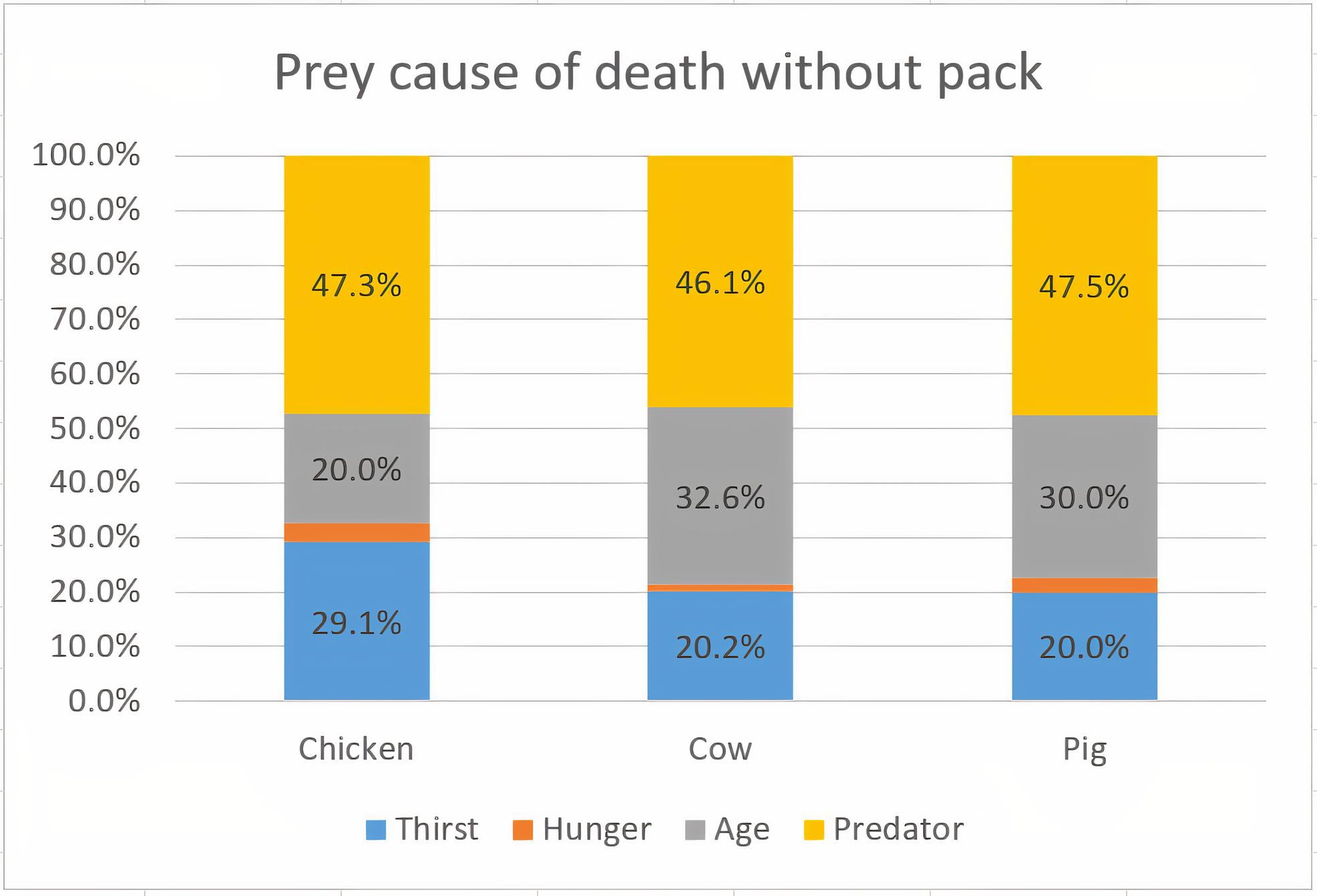
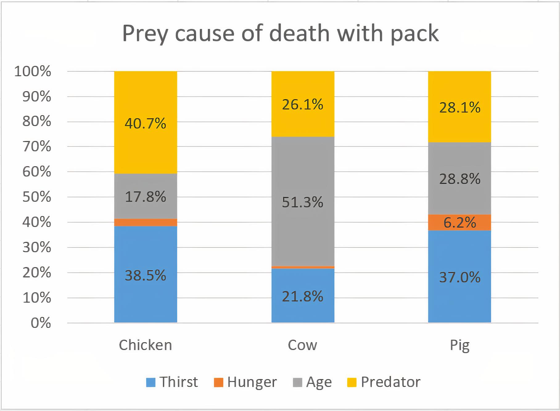
(a) Without pack

(b) With pack Figure 18: Vegetarian cause of death

As we can see in the above figure, the dispersion of predator death cases were drastically decreased.

Hypothesis 4 (H4): The food can decrease drastical ly near the pack’s area because of the many hungry mouth.

1. Considering the predator animals, this could depend on the hunting instinct. If a predator pack’s consumption is greater than a prey pack’s reproduction rate or multiple predator packs hunt the same prey pack it could be a disadvantage. Other than this situation, the pack’s survival rate is increased (shown in Hypothesis 2 and Hypothesis 3).

Animal Farm 81

2. Considering the prey animals, this hugely depends on the landscape’s layout and size. If the vegetation runs out in an area the pack will wander to a different area. This option is only available if the map’s size is big enough with few natural huge obstacle formations like oceans, mountains.

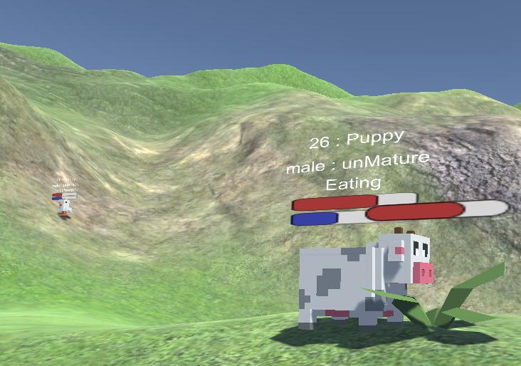
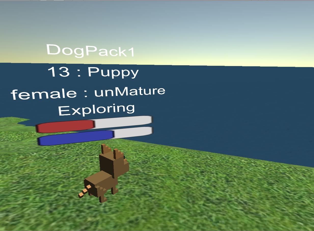
(a) High mountains

(b) Huge oceans Figure 19: Limitations of the land

10 Conclusion and future works

With the “Animal Farm” Framework, we created a simulation platform for everyone to run personal ecosystem simulations, with customizable animals in a simplified behavior and logic system. Running and observing this simulations, not only aesthetically beautiful, but generates ecosystem data in a large quantity. Using this data helps analyse and predict animal behaviours, extinction processes and any kind of change in the system on a wide variety (real and imaginary landscapes using heightmap data) of terrains. These kind of predictions can be very useful, when we run simulations of a real landscape terrain, with the replications of the animals living in that specific area, to observe and have a slight insight into the future of the real world’s ecosystem.

In the Framework, we are working on the implementation of more mechanics in animals’ behaviors, functionalities of the framework and monitoring, exporting and analysing more data for different experiments. The plan is to first upgrade and optimize some of the already implemented mechanics like a more complex calculation of the escape direction vector, where the animal takes into account all the enemies and their distances and calculates the appropriate summary vector instead of the closest enemy and reworking the animal’s view mechanic to a more optimized approach.

82 A. Kiss, G. Pusztai

We are also want to implement multiple new different mechanics, like a gene mechanic, which will influence the mating procedure, what kind of attractive attributes are the females and the males are looking for and whether they accept other ones approach or refuse them. Offsprings inherit different combinations of parental genes, also they can mutate a little the inherited gene pool at birth, taking evolutionary steps. We consider developing a role mechanic, which would mean, within the packs there could be different roles (such as hunter, explorer etc.) based on the animal’s outstanding abilities (using the gene system) to split jobs within packs. A hiding ability, smaller animals will be able to hide in specific locations (like bushes, nests) to escape from predators. New day-night cycles and sleeping mechanics. A family mechanic which represents a strong cohesion, like a pack, but this will be a closer bond, for example if a family member is in trouble, they will help immediately, the young ones may offer or share the food to the elder ones if they dangerously hungry. A basic form of communication (information transfer) between family, pack, race, to share location information like food and water location, dangerous areas and basic planned hunting process like attacking and surrounding the prey together. And an advanced fighting mechanic which replaces the current instant killing hunting mechanic of the predators. Introducing a new vitality meter (alongside the hunger and thirst) which shows, if the animal is full with energy (like not thirsty or hungry and not wounded) or lowered, because some causes, this will determine the damage they take and make to others. If taking damage or having a lower energy level, they start to suffer a penalty in attributes, like they will be reduced (e.g., the speed attribute will be lowered) until the energy reaches an optimal level and if the animal can keep it above this level the attribute will be slowly restored to the original value. With this new fighting mechanic, new battle types can be developed like intra-species struggles for food or females or during a hunt, a duel can take place where the prey can attacks back instead of just fleeing (creating a damage system, that takes down life force from both participants), where if one of the animal has a low life level he can decide to run away. Fellow animals nearby can help in the fight, if they decide to. This way not always the predators will win a fight if multiple preys unite to fight back and they kill or chase away a single predator.

Multiple functions are under consideration of adding, like an animal customization interface to create new animals and set the properties inside of the program. This custom created animals can be saved and spawned in simulations just like our 6 basic provided animals. New random/procedurally generated maps, using noises (Perlin [16] and other noise types merged) instead

Animal Farm 83

of using only heightmaps. For only entertainment we considered to implement one of the Unity’s VR (virtual reality) [7] functions into our simulation, to walk alongside of our animals and observe their behaviour closely, instead of just flying above them. If this implementation is successful and popular, we are considering adding additional functionalities like interacting with animals (human interference), where we could chase away predators or feed gentle animals and create farms with animals to experiment with the gene system or just testing our custom created animals.

We ran a large number of simulations, but the data gathering in the current framework wasn’t nearly complete. Only the ma jor statistics were monitored like number changes (every time something happened, the program logged the current statistic numbers) in the living (distributed by age stages) and the dead (distributed by death types) and the overall animal numbers in the whole simulations. We are planning to log and analyse more information like vegetation dispersion and monitoring vegetarian feeding habits, pack wondering patterns, influence of terrain formations (like hills and lakes) on the animals’ habits.

The “Animal Farm” Framework can be accessed on Github [25]. The system can freely be downloaded, extended and modified as a Unity pro ject for personal use. To try out and use a live version of the program without any installation, visit the browser version [26].

Acknowledgements

The pro ject has been supported by the European Union, co-financed by the European Social Fund (EFOP-3.6.3-VEKOP-16-2017-00002).

References

[1] C. Adami, C.T. Brown, Evolutionary learning in the 2D artificial life system

“Avida”, arXiv preprint adap-org/9405003, (1994). ⇒ 63 [2] H.R. Akcakaya, R. Arditi, L.R. Ginzburg, Ratio-dependent predation: an abstraction that works, Ecology, 76, 3 (1995) 995–1004. ⇒ 62 [3] A.A. Berryman, A.P. Gutierrez, R. Arditi, Credible, parsimonious and useful predator-prey models: a reply to Abrams, Gleeson, and Sarnelle, Ecology, 76, 6 (1995) 1980–1985. ⇒ 62 [4] F. Corno, E. Sanchez, G. Squillero, Exploiting co-evolution and a modified island model to climb the core war hill, The 2003 Congress on Evolutionary Computation, 2003. CEC’03, IEEE, 3, (2003) 2217–2221. ⇒ 63

84 A. Kiss, G. Pusztai

[5] J. Craighead, J. Burke, R. Murphy, Using the unity game engine to develop

SARGE: A case study, Computer, 4552 (2007). ⇒ 64 [6] C. Dachsbacher, M. Stamminger, Rendering procedural terrain by geometry image warping, Eurographics Symposium on Rendering (2004) 103–110. ⇒ 71 [7] J. Glover, Jesse J. Linowes, Complete Virtual Reality and Augmented Reality Development with Unity: Leverage the power of Unity and become a pro at creating mixed reality applications, Packt Publishing Ltd, 2019. ⇒ 83 [8] J.K. Haas, A history of the unity game engine, Worcester Polytechnic Institute, 2014. ⇒ 65 [9] D.G.Jones, A.K. Dewdney, Core war guidelines, Department of Computer Science, the University of Western Ontario, 1992. ⇒ 63 [10] M. Komosinski, The world of framsticks: Simulation, evolution, interaction, International Conference on Virtual Worlds, Springer, 2000, pp. 214–224. ⇒ 64 [11] M. Komosinski, Framsticks: A platform for modeling, simulating, and evolving 3D creatures, Artificial Life Models in Software, Springer, 2005. 37–66. ⇒ 64 [12] M. Komosinski, Sz. Ulatowski, Framsticks, Artificial Life Models in Software, 2007. ⇒ 64 [13] M. Komosinski, Framsticks, Artificial Life Models in Software, Springer, 2009. pp. 107–148. ⇒ 64 [14] M. Komosinski, et al., The Framsticks system: versatile simulator of 3D agents and their evolution, Kybernetes, MCB UP Ltd, 2003. ⇒ 64 [15] M. Komosinski, Sz. Ulatowski, Framsticks: Towards a simulation of a nature-like world, creatures and evolution, European Conference on Artificial Life, Springer, 1999. pp. 261–265. ⇒ 64 [16] H. Li, X. Tuo, Y. Liu, X, Jiang, A parallel algorithm using Perlin noise superposition method for terrain generation based on CUDA architecture, International

Conference on Materials Engineering and Information Technology Applications (MEITA 2015), Atlantis Press, 2015. ⇒ 82 [17] A. J. Lotka, Elements of Physical Biology, Williams and Wilkins Company, 1925. ⇒ 62 [18] K. Reddy, N. Ramacharyulu, A three species ecosystem comprising of two predators competing for a prey, International Conference on Simulation of Adaptive

Behavior, Springer, 2011. pp. 208–218. ⇒ 62 [19] T. Schmickl, K. Crailsheim, Bubbleworld. Evo: Artificial evolution of behavioral decisions in a simulated predator-prey ecosystem, Advances in Applied Science

Research, 2 (2006) 594–605. ⇒ 63 [20] S. Tom, Ray, An approach to the synthesis of life, Physica D, 1992. ⇒ 63 [21] Y.V. Tyutyunov, L.I. Titova, From Lotka–Volterra to Arditi–Ginzburg: 90 years of evolving trophic functions, Biology Bul letin Reviews, Springer, 10 (2020) 167–185. ⇒ 62 [22] V. Volterra, Leconssen la theorie mathematique de la leitte pou lavie, 1931. ⇒ 62 [23] R. Wiegert, G. Richard, Simulation Models of Ecosystems, Annual Review of

Ecology and Systematics, 1, 6 (1975) 311–338. ⇒ 62

Animal Farm 85

[24] L.Yaeger, Computational genetics, physiology, metabolism, neural systems, learning, vision, and behavior or Poly World: Life in a new context, Santa Fe

Institute Studies in the Sciences of Complexity, Addison-Wesley Publishing Co. 17 (1994). ⇒ 64 [25] ∗ ∗ ∗ Github pro ject repository, (2020), https://github.com/Wornox/AnimalFarmFramework. ⇒ 83 [26] ∗ ∗ ∗ Github runnable browser version of the program, (2020), https://wornox.github.io/AnimalFarmWebGL. ⇒ 83 [27] ∗ ∗ ∗ Unity (game engine), (2020), http://www.unity3d.com/. ⇒ 64 [28] ∗ ∗ ∗ Unity asset store, (2020), https://assetstore.unity.com/. ⇒ 66 [29] ∗ ∗ ∗ Unity asset: 5 animated Voxel animals by “VoxelGuy”, (2020), https://assetstore.unity.com/packages/3d/characters/animals/5-animatedvoxel-animals-145754. ⇒ 66 [30] ∗ ∗ ∗ Unity asset: Free Trees by ”AdaKing”, (2020), https://assetstore.unity.com/packages/3d/vegetation/trees/free-trees-103208. ⇒ 66 [31] ∗ ∗ ∗ Unity asset: Low Poly Nature - FREE Vegetation by ”Elcanetay”, (2020), https://assetstore.unity.com/packages/3d/vegetation/low-poly-nature-freevegetation-134006. ⇒ 66 [32] ∗ ∗ ∗ Unity asset: Runtime File Browser by ”yasirkulaa”, (2020), https://assetstore.unity.com/packages/tools/gui/runtime-file-browser-113006. ⇒ 66 [33] ∗ ∗ ∗ Unity asset: Voxel Animals Pack by ”VoxelGuy”, (2020), https://assetstore.unity.com/packages/3d/characters/animals/voxel-animalspack-133366. ⇒ 66

Received: January 8, 2021 • Revised: April 23, 2021