Breck School Advanced Science Research Journal


The Breck Advanced Science Research Program is the capstone course of the Breck science curriculum. This program gives students who are passionate about science and engineering the opportunity for an authentic, high-level summer research experience in collaboration with research professionals in universities, colleges or businesses.
Following the summer research component of the program, students participate in a year-long science research seminar class where they write and submit formal research papers and project presentations to the Twin Cities Regional Science Fair, Regional Junior Sciences and Humanities Symposium and the Minnesota State Science and Engineering Fair, with some students continuing on to the National Junior Sciences and Humanities Symposium or the International Science and Engineering Fair. In addition, Advanced Science Research students participate in a formal seminar at Breck where they present their work to family members, research advisors, and peers.
More information about the Breck School Advanced Science Research Program is available on our website: breckschool.org/asr
Dr. Kati Kragtorp, Director Advanced Science Research Program
Music and the Mind (Year Two)
the Intersection of Musical Proficiency and Reading Readiness
Noah DeMichaelis
Find Your Way
Design and construction of a multiple T-maze to assess spatial memory
Abigail Endres and Vivian Kinney
Problematic Packaging
Optimizing a method for dissolving alginate sheaths from cell fibers for 3D bioprinting
Anna Iordanoglou
Collision-Free Commutes
Designing a Blind Spot Detection System for Cyclists Using an Ultrasonic Sensor and Computer Vision
Noah Getnick and Evan Johnstone
Catching the Culprit
Western Blot Analysis of the Relationship Between Alzheimer’s Related Proteins
Aβ*56 and ΔTau303 in APP Transgenic Mice
Matthew Manacek and Samantha Dvorak
Deciphering DUX4
Is transient expression of the DUX4 gene sufficient to cause muscular dystrophy?
Corinne Moran
Refining the Ring Engineering nanobodies for a faster path to CSAN cancer immunotherapy
Charlotte Vasicek and Michael Setterberg
The Microplastic Butterfly Effect
Effects of dietary microplastic on survival and fitness of Cabbage White Butterflies (Pieris rapae)
Elin Wellmann
Use your mobile phone to scan the QR code included in each article to watch videos of our students’ presentations.
Noah DeMichaelis
Introduction
Reading is an essential skill for a successful future, and falling behind is catastrophic. The social ills of illiteracy emerge in a variety of ways, some seemingly unintuitive For instance, crime is significantly associated with illiteracy: 85 percent of juvenile delinquents are functionally illiterate (The Economic & Social Cost of Illiteracy, 2018). Additionally, illiteracy can impact health, since illiteracy limits a person’s ability to understand health information and increases the likelihood of high-risk sexual behaviors (The Economic & Social Cost of Illiteracy, 2018) Furthermore, the negative consequences of illiteracy are not strictly personal but can have large cumulative effects on society According to a 2018 report from The World Literacy Foundation Illiteracy costs the global economy 800 billion pounds (965 billion dollars) a year (The Economic & Social Cost of Illiteracy, 2018).
Research indicates a powerful association between rhythmic skills and pre-literacy in young children. In one study, preschoolers who were capable of mimicking a presented beat also exhibited greater proficiency in various preliteracy skills. These ‘synchronizers’, had greater phonological awareness (the ability to perceive and utilize spoken language), auditory short-term memory, and were quicker at naming presented colors or objects (Bonacina et al., 2018) These are all vital pre-literacy characteristics, and this data points towards an association between rhythmic ability and literacy skills The ability to keep a beat has also been shown to predict neural speech encoding in preschoolers. Beat synchronization reflects greater neural precision to temporal cues in speech (Woodruff Carr et al., 2014), which is associated with language acquisition and early

literacy Both adults and children who struggle to synchronize have deficits in neural encoding of sound and consequently reading ability (Kraus & Chandrasekaran, 2010)
Akin to the relationship between synchronization and reading, some research has also established a relationship between pitch and similar reading skills However, there is generally less research into this relationship, and often the research that exists presents a nuanced relationship Within the same study, among the two groups measured (third graders and daycare participants), pitch perception only correlated with phonemic awareness in the younger group, while rhythmic skills remained the strongest predictor of phonological and phonemic awareness (the ability to use and manipulate sounds in spoken language) among both groups (Steinbrink et al , 2019) Another study observed that children with learning disabilities (third through fifth graders) had poor pitch and rhythm proficiency as compared to children without learning disabilities (Lu et al , 2020) Indeed, many studies have seen a relationship between pitch-related musical skills and reading performance in children with dyslexia in particular (Fernández-Prieto et al., 2016; Foxton et al , 2003; Lu et al , 2020; Santos et al , 2007) It is likely that associations, if present, might only emerge in certain age ranges. Most studies demonstrating an association between pitch skills and reading skills tend to focus on younger children (Galicia Moyeda, 2017; Lamb & Gregory, 1993) However, Foxton et al (2003), observed a similar relationship between specific pitch-related skills and reading performance among an older age range (19-24 years old)
Whether or not pitch is a factor, research suggests that musical training could improve reading performance, while musical education
represents a potential remedy (Bonacina et al., 2021) Contrary to popular conception, musicality is not immutable Synchronization ability is shown to improve with practice. Musical training enhances auditory-motor development and is associated with superior reading ability (Steinbrink et al., 2019). Similarly, in one study, training in tonal-based musical training improved reading performance (Galicia Moyeda, 2017).
Rock ‘n’ Read is a Minnesota-based nonprofit founded to use music as a tool to strengthen reading. On the understanding that musical ability can be taught and that it presents benefits in other academic areas, Rock ‘n’ Read retrofitted city buses to include computers with ‘Tune Into Reading’ (a music-based educational software) to teach children to read through musical intervention. Through working with the program, participants saw significant gains in reading ability (Rock “ n ” Read Project, n d ) Motivated by such notable results, the organization decided to take their work even further and launched the “Zap the Gap'' campaign. Through their campaign, the Rock ‘n’ Read is emphasizing musical ability at very young ages (prenatal to 5 years old), arguing that addressing current shortfalls in reading ability through musical training can prevent deficits from becoming more pronounced over time To aid in this effort, Rock 'n’ Read produced a free musical fitness assessment (Musical Fitness Assessment, n d ) The musical fitness assessment measures proficiency in beat synchronization, and singing in tune, among other musical skills This assessment provides a simple, consistent measure of musical ability to help identify musical deficits in young children.
In the first year of this study (2022), I analyzed three sets of data collected from first-grade participants at Breck School, a suburban, independent school near Minneapolis, Minnesota: a parent/guardian survey on each participant’s past musical training, an assessment of their musical skills, and their most recent phonemic ability scores. Phonemic ability was determined through the Heggerty Guide-
lines for Scoring the 1st Grade Baseline Phonemic Awareness Assessment (The National Reading Panel Report, 2000) This phonemic awareness assessment tests rhyme production, onset fluency, blending phonemes, isolating final sounds, segmenting words into phonemes, isolating medial sounds, adding additional phonemes, deleting additional phonemes, and substituting initial phonemes The Musical Fitness Assessment covered skills including synchronization to a beat, syllable perception with a song, and singing in tune I found that pitch perception, along with syllable perception, had the highest correlation with phonemic awareness Early exposure to music education was linked with improved musical fitness, however, this was due to the association between increased early musical education and synchronization, while no such association was seen with pitch-related skills This was likely why there was no association between musical exposure and phonemic awareness. Exposure to music education was only linked with synchronization, not pitch, while only pitch, and not synchronization, was linked with phonemic awareness
These results were intriguing, but they also posed some new questions. The associations I noted between student scores on the Heggerty Phonemic Awareness Assessment and their pitch skills might have been an artifact of the specific type of reading-readiness assessment I looked at and not representative of a broader association between reading and pitch skills. The Heggerty Phonemic awareness assessment explicitly focuses on speech sounds, as opposed to written text, which may lead to it developing a stronger relationship with pitch, where no such relationship exists with reading as a whole It was also possible that the results observed in the 2022/2023 study may be a product of a small sample size (29) Given a larger sample size, previous trends could disappear, or new trends could develop.
In this second year of research, I investigated whether the Musical Fitness Assessment data collected in 2022 (year 1 of this study) correlates
with other reading-related measurements. Specifically, I investigated whether musical proficiency correlates with other reading metrics Additionally, I looked at what aspects of musical proficiency (pitch skills, rhythm skills, musical experience) drove this correlation and if this correlation was different than the relationship previously observed with the Heggerty Phonemic Awareness Assessment I repeated the assessment with a second cohort of first-grade participants to determine whether the relationship between pitch-related skills and reading proficiency remained consistent. I also developed and included additional measures of pitch-related skills in the Musical Fitness Assessment to determine whether these also correlated with reading readiness measures
2022/2023
In the spring of 2023, I obtained additional reading-related data from the children who participated in the first year of this study. An additional consent form was sent out to each parent or guardian of a first-grade student who had participated in the initial study. In total, 25 parents permitted us to access their children’s additional testing data A reading specialist collected data using four different assessments from the Formative Assessment System for Teachers (FAST): sight words, nonsense words, word segmentation, and Curriculum-Based Measurement (CBM). The sight word assessment tests the ability of first graders to read the 150 most prominent English words. The word segmenting portion of the test asks participants to separate spoken words into individual sounds In the nonsense word test, participants are asked to read as many phonetically regular nonsense words as possible in one minute The CBM asks participants to read as many words as possible from three texts without pictures in one minute. Sight words, nonsense words, and word segmentation were measured in the fall of 2023, while all four scores were collected in the spring of 2023
Using the online software, DataClassroom (Temple & Reedy, Aaron, n d ), I used linear regression to compare each new reading assessment score (sight words, word segmenting, nonsense words, and CBM) with last year’s data on the level of musical exposure and musical fitness assessment scores. I used the Mann-Whitney U Test to compare individual musical fitness skills with the new reading assessment scores.
The research participants in the 2023/2024 cohort were first-grade participants (ages 6-7) from Breck School in Golden Valley, MN Breck School is a suburban, independent, pre-K through grade 12 college preparatory school. This study represents an age, gender, and racial/ethnic composition representative of the first-grade student body at this institution. This study did not include any otherwise listed vulnerable populations An introductory email containing a link to an online Google Form survey was sent to all parents/guardians of 2023/24 first-grade participants at Breck School in the fall of 2023, inviting them to participate in the study Parents were recruited using printed flyers, email invitations, and tabling at school events. Consent and assent were collected through a Google form sent to the parents and guardians of the 2023 first-grade class
A link to an online Google Form survey was sent to all parents/guardians of incoming 2023/24 first-grade participants at Breck School in Golden Valley, MN Beginning with the consent and assent forms, the survey asked for information about their child, including years at Breck School, current age, amount, and type(s) of musical education before and after kindergarten. After parents/guardians concluded the survey, the data was anonymized by my mentor before being provided to me
Each participant was administered the Rock ‘n’ Read Basic Musical Fitness Assessment (Musical Fitness Assessment, n d ) with additional tone-discrimination questions. Participants were tested individually at their school during scheduled music class time or during scheduled morning meeting time by a member of the school faculty The musical assessment asked children to perform specific tasks including synchronization to a metronome, patting syllables of words with a song, vocally matching pitch, and singing in tune For the rhythm portion of the assessment, participants patted any relevant beats on their lap to provide more tactile stimuli statistically shown to improve rhythmic ability in children (Kuhlman & Schweinhart, 1999)
For this second year of data collection, I designed a tone-discrimination task, based on a previously published tone-discrimination task (Lu et al , 2020) and the Primary Measure of Music Audiation by Edwin E. Gordon (Primary Measures of Music Audiation, n.d.). Participants listened to a series of tone pairs and were asked to determine whether the pitch increased, decreased, or remained the same. The tone discrimination portion of the assessment had three sections that progressed in difficulty. Each section featured a question where the pitch increases, one question where the pitch decreases, and one question where the pitch remains the same. Pitches in the first section began on a middle C and increased or decreased by two whole steps. Pitches in the second section began with an E and only increased and decreased by one step Pitches in the third section began on a G and changed by only a half step. To protect anonymity, scores were de-identified before being provided to me
In the fall of 2024, the Breck school reading specialist collected reading assessment scores from the first-grade class. These reading scores included some of the same reading metrics collected in the 2022/2023 first-grade class: word segmenting, sight words, and nonsense
words. Notably, the Curriculum-Based Measurement (CBM) and the Heggerty Phonemic Awareness assessments were not administered in the fall of 2023.
Using the online software, DataClassroom, I assessed the relationship between the level of musical exposure, reading performance, and musical proficiency of the 2023/2024 first-grade class. I used linear regression to compare each new reading assessment score (sight words, word segmenting, and nonsense words) with scores and combinations of scores from the Musical Fitness Assessment These included Musical Fitness Assessment total, Pitch, Pitch + Syllables, and Synchronization + Syllables. I used the Mann-Whitney U Test to compare individual musical fitness categories with new reading assessment scores.
Additional fall testing data - 2022/2023 (Year I) cohort
In the additional testing data collected in the Fall of 2022, syllable scores had a significant, positive correlation with nonsense words score (p < 0.05; Table 1), but no other significant correlations were observed between fall FAST scores and musical fitness assessment scores Total Heggerty score had a significant positive correlation with nonsense words scores (p < 0 05; Table 1) but did not correlate with the other two reading assessments.
Additional spring testing data - 2022/2023 (Year I) cohort
In the additional testing data collected in the Spring of 2023, Musical Fitness Assessment total score did have a significant positive correlation with each FAST metric collected in 2023 (p < 0.05). Similarly, combined pitch matching and syllable scores had a significant correlation with Total Heggerty Score There was a significant positive correlation between Musical Fitness Assessment total score and all FAST assessment scores (p < 0 05; Table 2)
Table 1. Summary of Mann-Whitney, or (*) linear regression statistical analysis, of additional FAST fall testing data from 2022/2023 (Year I) cohort. Relationships with p < 0.05 are highlighted in yellow.
Table 2. Summary of Mann-Whitney, or (*) linear regression statistical analysis, of additional FAST spring testing data from 2022/2023 (Year 1) cohort. Relationships with p < 0.05 are highlighted in yellow.
Combined pitch score was significantly, positively related to the score on the sight words assessment (p < 0 05; Table 2) This was the only type of reading-related score collected in the spring of 2023 with a significant positive correlation with pitch performance in isolation (p < 0.05; Table 2). Similarly, beat- keeping scores in isolation only had a significant positive correlation with word segmenting
Sight word scores collected in the Fall of 2022 correlated significantly with sight word scores collected that Spring in 2023 (p < 0 01) Similarly, nonsense word scores collected in the Fall of 2022 correlated significantly with nonsense words collected in the Spring of 2023 However, word segmenting scores collected in the Fall of 2022 did not correlate significantly with word segmenting scores (p = 0 98)
2023/2024 (Year II) cohort comparison to 2022/2023 (Year 1) cohort
Compared to year one of this study, the number of participants in year two increased from 29 to 34 (Table 3) The percentage of students who received in-school pre-K musical education was 72% in year one compared to 38% in year two
This difference was statistically significant (p < 0.001). Similarly, the average level of musical exposure was 1 6 in year one (2022/2023) and 1.2 in year two (2023/2024); a statistically significant difference (p < 0.04; Table 3). There were no significant correlations between performance in any musical skill metric or level of musical exposure with scores on assessments of sight words, word segmenting, or nonsense words in the fall data from the 2022/2023 (Year I) cohort (data not shown).
Performance on the tone discrimination task ranged from a minimum of 11 to a maxi- mum of 18 out of 18 total possible points, with 47% of students earning full points on the task (Table 4). There was a significant correlation between performance on the second-tone-high question of the tone discrimination assessment and total musical fitness assessment score (p < 0.01). However, this significance was due to an individual participant who did not correctly identify any of the second-tone-same questions. When this outlier was removed, the relationship was no longer significant.
Additionally, there was a significant correlation between total musical fitness assessment score and performance on the one-step change portion of the tone discrimination activity (p < 0.03). However, this significance was due to the same individual outlier When the outlier was removed, the relationship was no longer significant There were no other significant correlations between performance on the tone discrimination task and any section of the musical fitness assessment There was no significant relationship between the tone discrimination task score and any of the FAST scores
Table 4. Summary of Performance on Tone Discrimination Activity
Mean Score +/- s.d (max score) % of subjects answering correctly
Total 15 9 +/- 2 7 (18) 47
Second tone Low 5.1 +/- 1.3 (6) 53
Second tone High 5.1 +/- 1.4 (6) 58
Second tone Same 5.6 +/- 1.2 (6) 88
Two-step change 5.5 +/- 0.9 (6) 74
One-step change 5.3 +/- 1.0 (6) 56
Half-step change 5.1 +/- 1.3 (6) 62
In the first year of this study, I found a significant, positive correlation between musical fitness and performance on the Heggerty Phonemic Awareness Assessment, with a highly significant positive correlation between combined scores for pitch perception and syllable awareness and the Heggerty score In this second year, I obtained and analyzed additional data from this cohort, which revealed that sight words, word segmenting, and nonsense
Noah DeMichaelis
word scores collected in the fall from this cohort did not significantly correlate with musical fitness assessment scores (except for syllable perception) or level of musical exposure. In addition, sight words, word segmenting, and nonsense word scores collected in the fall of 2022 did not correlate with Heggerty Phonemic Awareness scores collected in the fall However, FAST scores collected in the spring of 2023 had a significant, positive correlation with musical fitness scores, fall Hegg erty scores, and level of musical exposure Of the specific skills assessed in the musical fitness assessment, combined pitch and syllable scores had the strongest relationship with each aforementioned reading metric. Similar to the results for FAST reading scores collected in the fall semester for the year one cohort, in the year two cohort there was no association between musical proficiency and any of the fall FAST scores For the year two first-grade cohort, the Heggerty Phonemic Awareness assessment had been phased out by first-grade faculty in favor of the FAST assessment For this reason, it was not possible to compare the year one and year two cohorts regarding this metric This leaves a piece of potential data missing for this year’s study Similarly, it is too early to collect spring scores using the FAST assessment for the year two (2023/2024) cohort So, it remains to be seen whether the relationship observed between fall musical fitness assessment scores and spring FAST scores in the year one cohort repeats with the year two cohort.
This difference in the relationship between musical fitness assessment scores and FAST scores collected in the fall versus the spring semesters may stem from insufficient differentiation of FAST scores collected in the fall. Students learn to read at different rates, so over the school year, a greater range of FAST scores will develop The relationship between musical proficiency and reading readiness may develop over a school year because children themselves are developing
Performance on the new pitch discrimination questions was very high for the year two
(2023/2024) cohort, indicating the task itself was likely too easy for first-grade students This led to insufficient differentiation between first-grade participants to yield statistically significant results when compared with FAST assessment scores, or the musical fitness assessment scores, once a single outlier was removed. For this reason, in future assessments, it would be necessary to increase the challenge of this activity to gather more highly differentiated data.
In future investigations, it will be especially interesting to investigate how associations with different musical areas (pitch versus synchronization) and reading proficiency evolve as our tested population matures or as new participants are added. It may also be worthwhile to investigate whether musical intervention could improve reading proficiency, especially among the participants with the lowest scores on the FAST reading assessments. This investigation provides deeper insights into the dynamic between music and reading which may be useful in informing educational practices to help students best develop reading skills
Bonacina, S , Krizman, J , White-Schwoch, T , & Kraus, N (2018) Clapping in time parallels literacy and calls upon overlapping neural mechanisms in early readers: Clapping in time parallels literacy Annals of the New York Academy of Sciences, 1423(1), 338–348 https://doi org/10 1111/nyas 13704
Bonacina, S , Krizman, J , White-Schwoch, T , Nicol, T , & Kraus, N (2021) Clapping in Time With Feedback Relates Pervasively With Other Rhythmic Skills of Adolescents and Young Adults Perceptual and Motor Skills, 128(3), 952–968. https://doi org/10 1177/00315125211000867
Fernández-Prieto, I , Caprile, C , Tinoco-González, D , Ristol-Orriols, B , López-Sala, A , Póo-Argüelles, P , Pons, F , & Navarra, J (2016) Pitch perception deficits in nonverbal learning disability Research in Developmental Disabilities, 59, 378–386 https://doi org/10 1016/j ridd 2016 09 011
Foxton, J. M., Talcott, J. B., Witton, C., Brace, H., McIntyre, F., & Griffiths, T D (2003) Reading skills are related to global, but not local, acoustic pattern perception Nature Neuroscience, 6(4), 343–344 https://doi org/10 1038/nn1035
Galicia Moyeda, I X (2017) Influencia de un entrenamiento en discriminación de estímulos tonales en la conciencia fonológica de niños preescolares Estudio piloto / Influence of tonal stimuli discrimination in the phonologic awareness of preschool children. Pilot study RIDE Revista Iberoamericana Para La Investigación y El Desarrollo Educativo, 8(15), 529–547 https://doi org/10 23913/ride v8i15 309
Kraus, N , & Chandrasekaran, B (2010) Music training for the development of auditory skills. Nature Reviews Neuroscience, 11(8), 599–605 https://doi org/10 1038/nrn2882
Kuhlman, K , & Schweinhart, L J (1999) Timing in Child Development High/Scope Educational Research Foundation
Lamb, S J , & Gregory, A H (1993) The Relationship between Music and Reading in Beginning Readers Educational Psychology, 13(1), 19–27 https://doi.org/10.1080/0144341930130103
Lu, H , Zhang, K , & Liu, Q (2020) Reading fluency and pitch discrimination abilities in children with learning disabilities Technology and Health Care, 28, 361–370 https://doi org/10 3233/THC-209037
Musical Fitness Assessment (n d ) Rock “n” Read Project Retrieved May 27, 2022, from https://www rocknreadproject org/musical-fitness-assessment
Primary Measures of Music Audiation (n d ) https://www giamusic com/store/resource/primary-measures-of-mu sic-audiation-kgrade-3-complete-kit-pmma-instrumentaccessory-g 2242k
Rock “n” Read Project (n d ) Rock “n” Read Project https://www.rocknreadproject.org/new-programs
Santos, A , Joly-Pottuz, B , Moreno, S , Habib, M , & Besson, M (2007) Behavioural and event-related potentials evidence for pitch discrimination deficits in dyslexic children: Improvement after intensive phonic intervention Neuropsychologia, 45(5), 1080–1090 https://doi org/10 1016/j neuropsychologia 2006 09 010
Steinbrink, C , Knigge, J , Mannhaupt, G , Sallat, S , & Werkle, A (2019) Are Temporal and Tonal Musical Skills Related to Phonological Awareness and Literacy Skills? – Evidence From Two Cross-Sectional Studies With Children From Different Age Groups Frontiers in Psychology, 10, 805 https://doi org/10 3389/fpsyg 2019 00805
Temple, D , & Reedy, Aaron (n d ) DataClassroom DataClassroom. Retrieved November 20, 2023, from https://about dataclassroom com
The Economic & Social Cost of Illiteracy (2018) World Literacy Foundation https://worldliteracyfoundation org/wp-content/uploads/2021/07/T heEconomicSocialCostofIlliteracy-2 pdf
The National Reading Panel Report. (2000). https://heggerty org/Phonemic-awareness-research/
Woodruff Carr, K , White-Schwoch, T , Tierney, A T , Strait, D L , & Kraus, N (2014) Beat synchronization predicts neural speech encoding and reading readiness in preschoolers Proceedings of the National Academy of Sciences, 111(40), 14559–14564 https://doi org/10 1073/pnas 1406219111
Endres and Vivian Kinney
Abigail Endres and Vivian Kinney
Introduction
Spatial memory refers to the ability to store and manipulate spatial information and it allows one to create a mental representation of one’s surroundings (Johnson & Redish, 2007; Morellini, 2013) This representation of space is what allows individuals to navigate through space. Spatial memory is used for everyday tasks such as navigating home through a familiar city Spatial memory is also impacted by neurodegenerative diseases, like Alzheimer’s disease (AD) The initial stages of AD include many spatial memory deficits, such as spatial disorientation. In fact, over 60% of AD patients suffer from spatial memory deficits (Silva & Martínez, 2023). Understanding spatial memory is integral to comprehending the fundamental mechanisms underlying human cognition
Much research has been conducted on the role of the hippocampus in spatial memory in binding together distributed sites in the neocortex to represent a whole memory (Eichenbaum et al , 1999). It is understood that the sequential firing of the hippocampus plays an important role in encoding spatial information Place cells, located within the hippocampus, associate a landmark or location with a cell to create a representation of space (Silva & Martínez, 2023) Still, there is much that is not known about how different brain regions interact and coordinate their activity during the process of spatial memory, due to the sheer complexity of the brain (Robin et al , 2015)
One way that researchers study spatial memory in mice is through a behavioral paradigm called the T-maze The T-maze requires the mouse to navigate its surroundings, testing the mouse’s ability to retain spatial information (Deacon & Rawlins, 2006) A basic T-maze consists of a

stem that guides the mouse forward to the decision point where the mouse is forced to choose between a left or right turn The mice are trained to learn that one choice is programmed with a reward After a sufficient amount of training, the mice are then given full, free choice between the two sides. The choice the mice make is then recorded In each trial, the mouse loops through the T-maze multiple times so that an adequate amount of data is collected. However, since this maze is not continuous, the mouse has to be physically removed from the maze, which causes the mouse to become stressed The single decision point in a standard T-maze limits the complexity of the maze and fails to properly challenge the mouse.
Most work in understanding brain region connectivity is limited to head-fixed mice, which does not adequately model what is happening in the brain of a mouse freely moving around in its environment A recent advancement in brain imaging technology is the development of cortical-wide imaging devices for mice, called the “Mini-MScope” (Donaldson et al , 2022; Rynes et al., 2021). These devices are miniaturized head-mounted imaging microscopes that allow for the recording of cortical-wide activity in freely behaving mice that have been genetically modified to possess the Thy1-GCaMP6f gene (GCaMP) The GCaMP gene activates a green fluorescent light when neurons fire, allowing for the recording of neural activity
We developed a modified T-maze to analyze cortical-wide activity, using Mini-MScope technology, as mice completed a task that challenged their spatial memory. We included two T decision points in our maze to observe differences in brain activity and connectivity during spatial memory tasks. The maze was
made to be continuous to allow for multiple, sequential trials This maze can be used as a tool to gain a deeper understanding of spatial working memory.
Materials and Methods
Maze design and prototyping
The initial maze design was developed using the Solidworks (Dassault Systemes) computer-aided design (CAD) The first three prototypes were constructed with cardboard and duct tape. 12 in. by 24 in. acrylic sheets were cut using a laser cutter to construct the maze and a hand file was used to file down any sharp edges. To create longer pieces, holes were drilled into the acrylic sheets and 3D-printed pieces were used to bolt sheets of acrylic together to create the desired length. Other 3D-printed pieces were created to act as the joints in the maze The doors were designed on Solidworks and were then 3D-printed. Servo motors were mounted on the walls of the maze using 3D-printed mounts 3D-printed doors were then attached to the servo motors. Infrared beam break sensors were also used in the construction of the final maze A combination of a syringe, tubing, and a DC motor were used to create a water dispenser. The motors and infrared beam break sensors were connected, controlled, and powered by an Arduino Due and an Arduino Mega system. The maze’s electronic system was created through the use of soldering equipment to connect the electronic components to power.
Mouse husbandry and handling
All mice used in this study we re housed in and handled by the Biosensing Biorobotics Lab in the University of Minnesota’s Mechanical Engineering Program according to an approved IACUC procedure. The authors were not in direct contact with the mice at any time Five male, Thy1-GCaMP6f, mice were used for their genetically modified calcium indicators that are expressed in layers 2, 3, and 5 of the cortex The mice had been fitted with a clear ‘cap’ (the e-SeeShell) that allowed for the observation of brain activity using the Mini-MScope Mice
were surgerized for previous research that had since finished and were not prepared specifically for our research
To increase motivation during the behavioral task, the mice were water-restricted using a procedure already in place for other research being performed in the lab. All water restrictions performed complied with IACUC guidelines. Mice were housed in a 14-hour light /10-hour dark cycle. For this project, the effects of water restriction on a navigation task were studied in mice by looking at brain activity and animal behavior. RAR staff were notified of mice under water restriction and daily body weight was taken for each mouse under water restriction protocols. Trained researchers closely monitored water restriction effects, which was conducted over a 10-day period, by examining mouse locomotion and posture during daily interaction sessions.
The dimensions of maze design I were 40 in. by 34 in and consisted of two basic T decision points that led to an outer path that contained a reward on the lateral sides (Figure 1). A door was placed on the left side of the first T to force a right turn The initial plan was to have cues to signal what direction the mice should turn at the second T The second T held the central choice zone, which was the point where the mice made the turn that would lead them to the reward. Doors at either end of the secon d T would close after the mice had made their final choice When the mice move along the outer path, they would be led back to the starting point and continue to cycle through the maze
Abigail Endres and Vivian Kinney
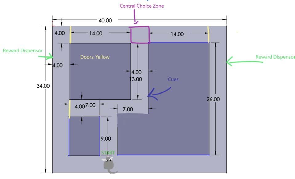
Figure 1. Annotated image of design I. The Solidworks design of the initial prototype, including annotations of electronic elements of the maze. Figure by authors.
A prototype of the first maze design was constructed out of cardboard (Figure 2) After consultation with researchers, it appeared that the maze was too short. An increase in the length of the maze was recommended because if the mice exert more energy completing the trials, they are more likely to pause at the central choice zone
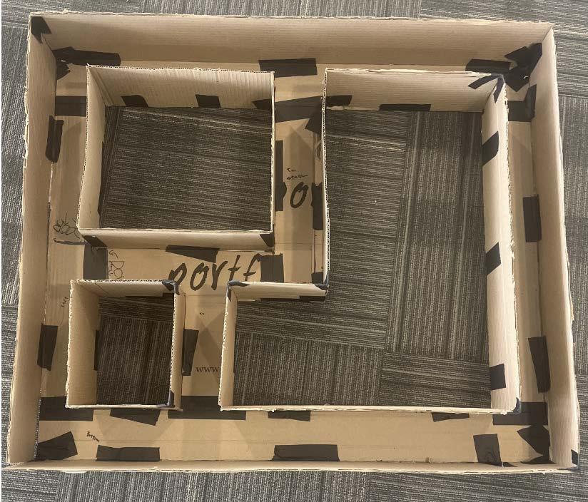
2. Cardboard prototype of maze design I. An image of the maze prototype I which was constructed out of cardboard. Figure by authors.
The dimensions of maze design II were 36 in. by 36 in and consisted of two basic T decision points that led to a winding outer path that
contained a reward on the lateral sides (Figure 3) The door by the first T decision point in maze design I was replaced by a wall After consultation with researchers, it appeared that this maze design was too complex The winding outer path would lead the mice to become disoriented and unable to complete the maze.
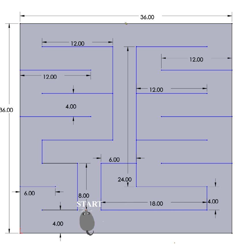
Figure 3. Annotated image of maze design II. The Solidworks design of the second prototype, including annotations regarding the start point Figure by authors
The dimensions of maze design III were 72 in by 72 in and consisted of two basic T decision points that led to a curved outer path that extended through the length of the entire maze and contained a reward on the lateral sides (Figure 4). After consultation with researchers, it was concluded that this maze design would likely work My partner and I then determined that we should first scale the maze down before prototyping to be mindful of the space and material that would be used
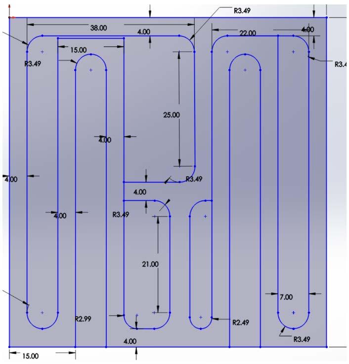
Figure 4. Image of maze design III. The Solidworks design of the third prototype. Figure by authors.
Maze Design IV
The dimensions of design IV were 48 in. by 48 in and consisted of two basic T decision points that led to an outer path that extended through the length of the entire maze and contained a reward on the lateral sides (Figure 5)
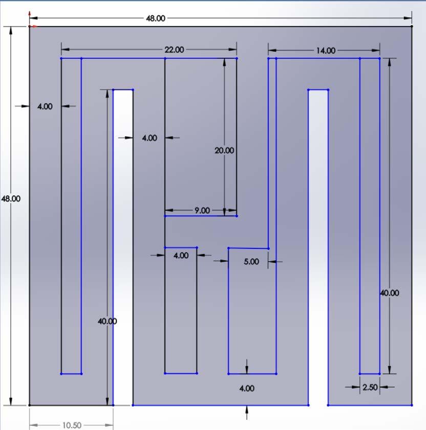
Figure 5. Image of maze design IV. The Solidworks design of the fourth prototype Figure by authors
Maze Prototype IV
A prototype using the dimensions of the fourth maze design and the curved element of the third maze design was constructed out of cardboard (Figure 6). After consultation with researchers, it was recommended that we increase the length of the first T’s choice paths to ensure that the mice would be sufficiently challenged at that decision point
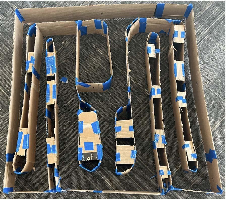
Figure 6. Cardboard prototype of maze design IV. An image of the maze prototype IV which was constructed out of cardboard Figure by authors
Maze Design V
The dimensions of maze design V were 48 in by 60 in. and consisted of two basic T decision points that led to a winding outer path that contained a reward on the lateral sides (Figure 7). After consultation with researchers, it was recommended that we make the maze more symmetrical to ensure that the distance traveled wouldn’t influence the direction the mice would choose
Abigail Endres and Vivian Kinney

Figure 7. Image of maze design V. The Solidworks design of the fifth prototype. Figure by authors.
Maze Design VI
The dimensions of maze design VI were 48 in. by 60 in and consisted of two basic T decision points, with a sharp turn in between, that led to a winding outer path that contained a reward on the lateral sides (Figure 8)

Figure 8. Image of maze design VI. The Solidworks design of the sixth prototype Figure by authors
Maze Prototype VI
A prototype of the sixth maze design was constructed out of cardboard (Figure 9). Researchers directed untrained and unmotivated mice through the cardboard maze and determined that the maze was effective. It was recommended that unnecessary gaps in the maze be removed to limit the material used in the final design.

Figure 9. Cardboard prototype of maze design VI. An image of the maze prototype six which was constructed out of cardboard. Figure by authors.
Final Maze Construction
The final maze was constructed using ¼ inch white acrylic The maze dimensions were 39 in by 56 5 in and the walls were 6 in high (Figure 10). The acrylic pieces were connected with 3D-printed joints and some boards were elongated with the use of 3D-printed pieces and bolts. The maze contained five servo motor-controlled doors that were activated through the use of infrared (IR) beam break sensors, and one water-reward station.
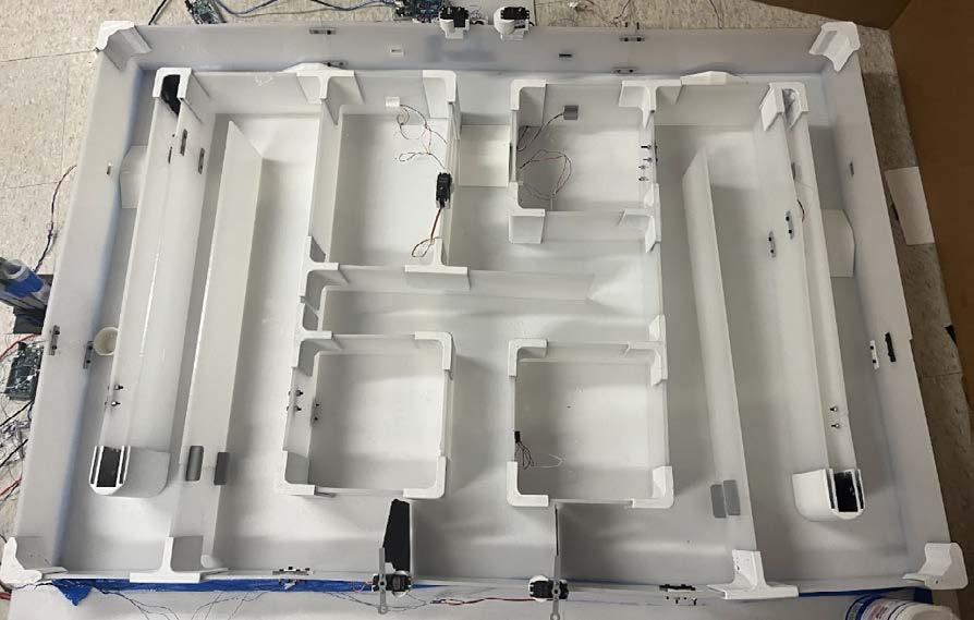
Figure 10. Final maze. An image of the final maze Figure by authors
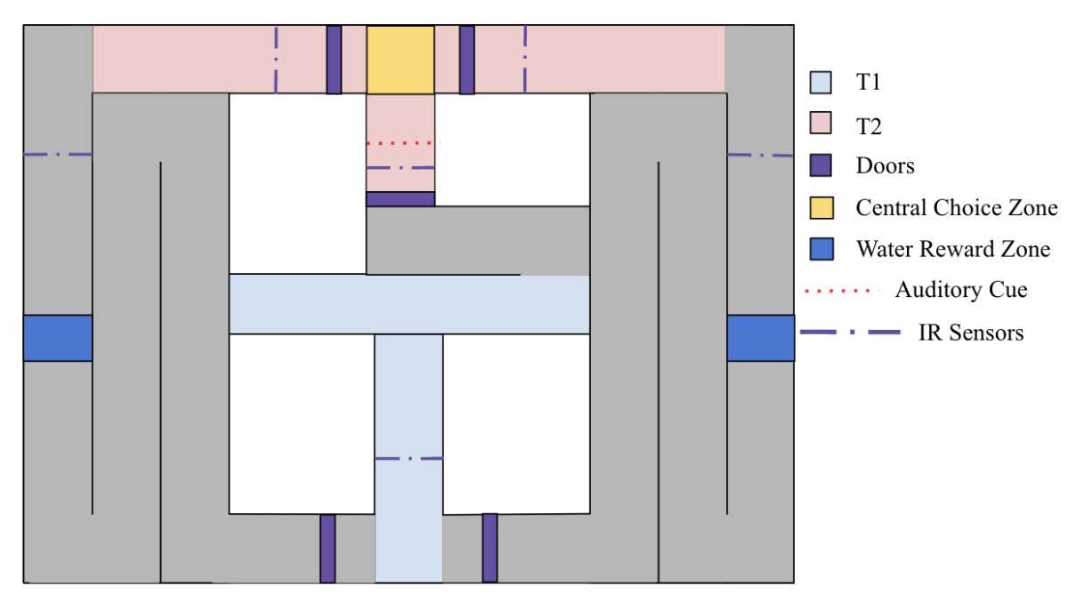
Maze Route
At the start of each trial, a mouse was placed at the first T and then directed to complete the maze (Figure 11) The first T decision point the mice encountered required them to make a right turn to continue through the maze. Once the mice had made the right turn, they entered the stem of the second T At the second T, the mice
reached the central choice zone where they were required to make a left or right turn To ensure brain data could be measured as the mice made that choice, the IR beam break sensors closed servo motor-controlled doors This enclosed the mice in the central choice zone to force a pause During that pause, an auditory cue was played to inform the mouse whether to turn left or right After a delay, the doors opened and the mouse was free to move forward. Once the mice had made a choice, t he door would close behind them to help direct them If the mice made the correct choice, they received a water reward from a dispenser Once the mouse had completed their trial, they were returned to their cage.
After an initial behavioral trial, a few issues were identified. First, the mice were not tall enough to trigger the sensors so ramps were 3D-printed. The addition of these ramps led to the placement of the doors to shift to ensure that the doors would not trigger the sensors. To minimize the risk of our electronics burning out, an additional Arduino system was added. To close the doors near the starting point sooner, another sensor was added through the use of a drill and double-sided tape. The auditory cue was removed from the maze due to the observations of researchers who were currently
attempting a similar training process on a different project. Instead, the mice were trained to associate one side of the maze with the water reward The mice were then tested on their ability to identify which turn would lead to a reward
Five transgenic mice were used during an eight-day training and experimentation period. For the first five days, the mice were introduced to half of the maze This time was to help the mice acclimate to the maze and have them associate the right-hand turn with the water reward On days 6 and 7, the mice were introduced to the other half of the maze. The mice were forced to do alternating left and right turns while getting rewarded with water on the right side only. After only a few laps, the mice stopped checking for water on the left side of the maze On the final day, the mice were given full free choice to go left or right. Data was collected regarding whether the mice correctly identified which direction they should turn, as well as the time stamp. On average, the mice made both correct choices 71% of the time, which is close to the ~75% accuracy previously reported for mice running a simple T-maze (Pioli et al., 2014). Overall, this data demonstrates that the maze performed as expected
Abigail Endres and Vivian Kinney
Table 1. Percentage and number of correct decisions made by mice during final trials.
Mouse % of correct choices on T1 (# correct/total trials) % of correct choices on T2 (# correct/total trials) % of both correct
1 86% (6/7) 83% (5/6) 83% (5/6)
2 83% (10/12) 75% (9/12) 67% (8/12)
3 100% (7/7) 86% (6/7) 86% (6/7)
4 86% (6/7) 86% (6/7) 86% (6/7)
5 56% (5/9) 78% (7/9) 33% (3/9)
Limitations and Future Work
The number of mice that participated in the experiment was quite small. A larger sample would allow for more confidence in the results of the experiment Despite rounding the 3D-printed joints, the wires attached to the Mini-MScope still often got caught on the joints In the future, the creation of a joint design that is more flush with the maze could help prevent this problem In addition to the behavioral data collected, the Mini-MScope technology allowed for the collection of brain imaging data. This data is still in the process of being analyzed, but we hope that it will provide significant insight into brain activity. Further iterations of this maze will allow for a better understanding of spatial memory and could eventually lead to earlier diagnosis, disease prevention, and even treatments for memory-altering diseases
We would like to thank Dr Kati Kragtorp for her support throughout the project. We would also like to thank Dr Suhasa Kodandaramaiah, from the Biosensing and Biorobtics Lab at the University of Minnesota, for granting us the opportunity to perform this research Finally, we
would like to thank Daniel Surinach for overseeing us and helping us out throughout our research.
Deacon, R , & Rawlins, J (2006) T-maze alternation in the rodent Nature Protocols, 1, 7–12 https://doi org/10 1038/nprot 2006 2
Donaldson, P D , Navabi, Z S , Carter, R E , Fausner, S M L , Ghanbari, L., Ebner, T. J., Swisher, S. L., & Kodandaramaiah, S. B. (2022) Polymer Skulls With Integrated Transparent Electrode Arrays for Cortex‐ Wide Opto‐ Electrophysiological Recordings Advanced Healthcare Materials, 11(18), 2200626
https://doi org/10 1002/adhm 202200626
Eichenbaum, H , Dudchenko, P , Wood, E , Shapiro, M , & Tanila, H (1999) The Hippocampus, Memory, and Place Cells: Is It Spatial Memory or a Memory Space? Neuron, 23(2), 209–226. https://doi org/10 1016/S0896-6273(00)80773-4
Johnson, A , & Redish, A D (2007) Neural Ensembles in CA3 Transiently Encode Paths Forward of the Animal at a Decision Point Journal of Neuroscience, 27(45), 12176–12189 https://doi org/10 1523/JNEUROSCI 3761-07 2007
Morellini, F. (2013). Spatial memory tasks in rodents: What do they model? Cell and Tissue Research, 354(1), 273–286 https://doi org/10 1007/s00441-013-1668-9
Pioli, E Y , Gaskill, B N , Gilmour, G , Tricklebank, M D , Dix, S L , Bannerman, D , & Garner, J P (2014) An automated maze task for assessing hippocampus-sensitive memory in mice Behavioural Brain Research, 261, 249–257 https://doi.org/10.1016/j.bbr.2013.12.009
Robin, J , Hirshhorn, M , Rosenbaum, R S , Winocur, G , Moscovitch, M , & Grady, C L (2015) Functional connectivity of hippocampal and prefrontal networks during episodic and spatial memory based on real-world environments: HPC and PFC Connectivity During Episodic and Spatial Memory Hippocampus, 25(1), 81–93 https://doi org/10 1002/hipo 22352
Rynes, M. L., Surinach, D., Linn, S., Laroque, M., Rajendran, V., Dominguez, J , Hadjistamolou, O , Navabi, Z S , Ghanbari, L , Johnson, G W , Nazari, M , Mohajerani, M , & Kodandaramaiah, S B (2021) Miniaturized head-mounted microscope for whole cortex mesoscale imaging in freely behaving mice Nature Methods, 18(4), 417–425 https://doi org/10 1038/s41592-021-01104-8
Silva, A., & Martínez, M. C. (2023). Spatial memory deficits in Alzheimer’s disease and their connection to cognitive maps’ formation by place cells and grid cells Frontiers in Behavioral Neuroscience, 16, 1082158 https://doi org/10 3389/fnbeh 2022 1082158
Optimizing a method for dissolving alginate sheaths from cell fibers for
Anna Iordanoglou
Introduction
As many as 17 people die per day in the US while waiting for an organ transplant (6 Quick Facts About Organ Donation, n.d.). A lack of donors is only part of the issue. Organs for a transplant must be removed from a recently deceased person and given to the patient awaiting a donor within a certain increment of time 36 hours is the longest the kidney can be preserved before being transplanted, and a heart can only remain outside a human body for around 6 hours (Learn How Organ Allocation Works - OPTN, n.d.). A further issue is that the organs must be undamaged for them to work. Compatibility is another issue, as only one specific tissue type or blood type will work for a given person. If humans could print organs for patients using their tissue, many lives would be saved.
3D bioprinting is a way to artificially create tissue from living cells that can function as natural tissues (Pushparaj et al , 2023) Eventually, these tissues could be used to create organs for transplants In standard 3D printing, layers of filament are stacked on top of each other to create a three-dimensional object. 3D bioprinting works similarly, except it utilizes ‘bioink’ to create the designs and models Bioink is made up of living cells within a matrix of synthetic or natural biomaterials, or a combination of the two (Gungor-Ozkerim et al , 2018). Theoretically, bioink should be able to exactly replicate human tissue (Pushparaj et al , 2023) A 3D bioprinter then uses software to follow a predetermined design, like regular 3D printers, and extrudes the bioink in a pattern that will emulate the structure and function of tissue
Anna Iordanoglou

The 3D Bioprinting Facility at the University of Minnesota is currently developing a protocol to print the Gastroesophageal Junction (Gej). The Gej is the valve between the stomach and esophagus, made up of smooth muscle cells Its role is to stop acid from the stomach from entering the esophagus. If not functioning properly, it can result in inflammation, known as Gastroesophageal Reflux Disease (GERD; Kahrilas, 1997). In severe cases, GERD also progresses to esophageal cancer (Vogt & Panoskaltsis-Mortari, 2020). While there are treatments for the symptoms that stem from acid reflux, there is no way to actively repair a damaged Gej and address the root of the problem.
3D bioprinting a Gej is challenging due to the different directionality of the muscle cells in the Gej tissue. There are two main components to the Gej: the muscles that make up the esophagus and the muscles that make up the stomach. These two muscle types in the Gej, also referred to as the lower esophageal sphincter (LES), allow it to serve as a guard ring of muscle, protecting the lower opening of the esophagus (Vogt & Panoskaltsis-Mortari, 2020) Both the lower esophagus and the stomach are made up of smooth muscle cells (Hafen & Burns, 2023; Mittal, 2011) If these smooth muscle cells are not aligned properly, they are unable to create force.
The Panoskaltsis-Mortari lab is developing an aligned smooth muscle cell fiber (ASMSF) that could allow 3D bioprinting of Gej smooth muscle tissue (Panoskaltsis-Mortari, unpublished data) The fiber keeps smooth muscle cells aligned inside of the bioink. The ASMCF is made out of three parts: a sheath of calcium
chloride, a shell of alginate (a polysaccharide derived from brown algae), and a core consisting of collagen and smooth muscle cells (Figure 1) The alginate surrounding the core protects the collagen and cells from shear stress forces while the fiber is being made However, the alginate must be dissolved away from the ASMCF before being put into bioink, as it is not a natural component of human organs The gel around the fiber also needs to be dissolved as quickly as possible, because cells would be harmed in prolonged exposure to non-sterile environments
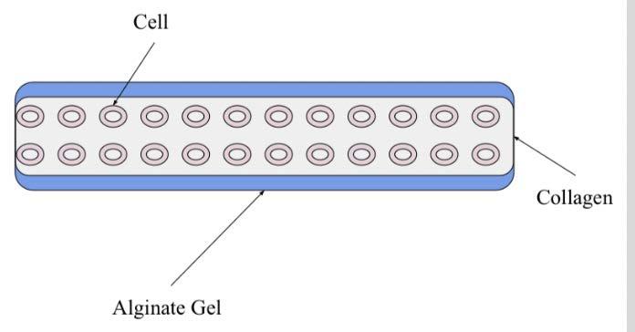
Figure 1. ASMCF diagram depicting the smooth muscle cells embedded in collagen and surrounded by the alginate gel. Figure by author.
Alginate is a polysaccharide extracted from brown algae. Sodium alginate in particular is made up of two acids, d-mannuronic (M units) and l-guluronic (G units), and it has a linear structure. One of the useful properties of alginate is its ability to interact with cations, mainly calcium, to form a strong gel (Abka-khajouei et al., 2022). This gel can be reverted to a liquid by two methods. One method involves using a calcium chelator a chemical that binds to the calcium in the gel to pull out calcium from the alginate’s structure (New Technique Turns Alginate Solution Into Micron-Scale Gel Patterns Using Light, n.d.). The second method involves an enzyme that degrades alginate by cleaving the glycosidic bonds and produces oligosaccharides (Zhu & Yin, 2015).
The procedure currently used by the Panoskaltsis-Mortari lab to dissolve the alginate in an ASMCF entails exposing the fiber to a 0.4 μg/ml alginate lyase enzyme solution However, full dissolution of the alginate takes an hour,
which is not fast enough to maintain cell viability Alginate lyase degrades alginate by cleaving glycosidic bonds via a beta elimination mechanism (Zhu & Yin, 2015), breaking the alginate down into oligosaccharides Ethylenediaminetetraacetic acid (EDTA) is a chemical that can also be used to dissolve alginate, because it pulls out the calcium that is used to crosslink alginate and turn it into a gel (Kiviranta et al., 1980). Like alginate lyase, EDTA is nontoxic to cells, and, thus, could be potentially useful in this application (Schubert et al., 2020).
My engineering goal was to determine the most efficient way to dissolve alginate from the ASMCF fiber without harming the cells. I tested the speed and effectiveness of alginate lyase, EDTA, and the combination of the two, in various concentrations, on the dissolution of alginate. Fluorescent dye was incorporated into crosslinked alginate beads to measure the diameter of the beads as the dissolution experiments were in progress. Once the most efficient method of dissolving alginate was determined, a replica of the fiber containing just the alginate on the outside and collagen in the core without cells present was used to gauge a more accurate time frame of when this method would dissolve the actual fiber. Although 0.1 M EDTA was the most efficient way to dissolve the alginate around the mock aligned fiber, EDTA in higher molar concentrations degraded the collagen inside the fiber Encouragingly, even this high level of EDTA was not toxic to the cells. Thus, the combination of alginate lyase and EDTA in a smaller concentration is a superior option.
Initial preparation of alginate beads
A concentration of 1 5% sodium alginate was used for creating the beads. This solution was created by dissolving 15 mg/ml of sodium alginate powder (Sigma Aldrich) into a sterile saline solution (11.237g of NaCl per liter of DI H2O). To ensure the alginate powder was equally distributed among the saline, it was put into a
Initial EDTA and Alginate lyase comparison tests
Alginate lyase was dissolved in Dulbecco's phosphate-buffered saline (DPBS) to create a stock solution of 100x alginate lyase. To ensure a homogenous mixture of DBPS and alginate lyase, the mixture was placed in a centrifuge This solution’s 100x concentration was 0.04 mg/ml of alginate lyase, and it was further diluted in DPBS to make 1x, 2x, and 5x solutions.
EDTA solutions were created at concentrations of 0 1 M, 0 15 M, and 0 2 M This was done by dissolving EDTA (Sigma Aldrich) into saline solution and heating slightly in a glass beaker with a stir bar functioning at medium speed until the EDTA was fully dissolved and the solution appeared clear. EDTA solutions were titrated using 10 M sodium hydroxide (NaOH) and 1 M hydrochloric acid (HCl) to achieve a pH range of 7.2-7.4, using a digital pH meter.
combination of alginate lyase and EDTA, also own as Emboclear, was created using blished procedures (Barnett & Gailloud, 11). 5 mg/ml of EDTA in saline was titrated ing sodium hydroxide 10 M (NaOH) and drochloric acid 10M (HCL) to a pH of 7 24. Then, alginate lyase powder was added to e solution at a concentration of 2 mg/ml
r the dissolution tests, 2-3 alginate beads were ded to each well of a 12-well plate, and melapse images were captured of each bead set ery five minutes for two hours for alginate ase tests and Emboclear tests, every two nutes for EDTA tests, until the beads were ssolved This imaging was done using the API setting of the EVOS-fl-auto-2 microscope. e Image stitching setting on the VOS-fl-auto-2 microscope was used in order to t the full view of each individual 12-well ate.
fining the imaging scan/bead preparation system was designed and assembled to create iform alginate beads small enough for microscopic analysis First, a 3D-printed structure was designed to hold a 5 ml syringe in place at an angle of exactly 55 degrees This angle was determined by taking a photo of the original bead-making process and using the ruler function on the iPhone photo software to determine the angle at which the ruler was being held to create beads with the smallest diameter possible
Solidworks was used to configure the design of the structure Slic3r was the software used to convert the design to instructions for the 3D printer to make the print The instructions were put into the Ultimaker 2 extended plus and the structure was printed.
A syringe pump was set to a rate of 1 5 ml/min, and a 32 gauge tip was attached to tubing between the opening of the syringe and the tip Once the syringe was placed inside the syringe pump, the tubing in between the syringe and the 32 gauge tip was woven through the structure 3D printed, in order to achieve the optimum droplet-making angle at 55 degrees. The syringe
pump was turned on and allowed to run for a time window of 3 to 5 minutes A 50 ml beaker of calcium chloride solution was placed under the syringe tip so the alginate would fall in and become crosslinked by the calcium
20 μl of 0 1 μm fluorescent microbeads (FluoSpheres™ Size Kit #2, Carboxylate- modified Microspheres, yellow-green fluorescent [505/515], 2% solids, Thermo Fisher Scientific) was added per one ml of 1.5% sodium alginate solution to facilitate measurement of the diameter of the alginate beads Beads were covered to reduce light exposure after being added to the alginate in a biosafety cabinet. The solution was vortexed after the microbead addition to ensure even dispersion of the microbeads.
Agarose gel molds were created to hold beads in place for the imaging scan, to ensure maximum accuracy of diameter measurements postimaging Using the software Solidworks, stamps in the shape of a circle with a diameter of 1 cm, with nine 3 mm deep rectangles that were 1.5 mm wide and 2 mm long protruding from the circular base, were created using a resin 3D printer. Once the design was configured on Solidworks, it was transferred to the software called Slic3r and converted to a stereolithography (STL) file and sent to the resin printer Once the design was printed, the stamps were cleaned with isopropyl alcohol (IPA) and then allowed to cure for an hour (Figure 3).
To create the agarose gel for the bead holders, saline (11 237g/L of NaCl/50ml) was placed into a 100ml beaker and set to warm up on a hot plate. Once the saline was warmed up, 2 g of agarose was added in slowly The heat was turned to a higher setting and the mixture was left on the hot plate until the particles of agarose dissolved Once the liquid was clear, the heat and stir settings were turned off, and 1 ml of agarose so lution was added to each well in a 12-well plate The stamps were placed into the warm agarose mixture and the well plate was placed at 23 ℃ until the agarose solidified into a gel The stamps were removed once the agarose was solid
Bead imaging procedure
Beads were imaged using an EVOS-fl-auto-2 microscope (ThermoFisher Scientific) Imaging areas were created for the scan procedure using the EVOS software. This was done by turning on the grid function and moving the position of t he microscope so that one of the wells created by the agarose mold was fully visible in the imaging window screen Then, aided by the grid function, the center of the imaging window screen was selected Once this center was selected, the button marked select image location was pressed to save that location. This was done for the top three of the nine well plates in each of the bigger twelve well plates The scan procedure was saved automatically before each experiment The GFP fe ature of the microscope was turned on during testing to visualize the fluorescence of the microbeads.
To calculate the rate of dissolution of alginate, the images of the beads were uploaded to Image J, and the straight line feature was used to measure the diameter of each bead for every time window when pictures were taken
EDTA and Alginate lyase refined comparison test
For the dissolution tests, three alginate beads were placed into every well of a 12-well plate with the bead holders. Timelapse images were captured of each bead set every five minutes for two hours for alginate lyase tests, and every two
minutes for EDTA tests, until the beads were dissolved The EDTA and alginate lyase combination was not used during this round of testing. GFP lighting in combination with DAPI lighting was used to capture the best possible images of the beads
Fiber tests were conducted using 0.1 M, 0.05 M, and 0 025 M EDTA alone Initial testing was done on the fibers surrounded in alginate, with no cells inside. The spun fibers were cut with a razor blade into 2 mm sections The fibers were placed into a 96-well plate, with no more than 12 fiber pieces in each of the well plates in order to not overcrowd the imaging scan Images were captured until the fibers had appeared to dissolve The Image stitching setting on the EVOS-fl-auto-2 microscope was used in order to get the full view of each individual 96 well plate.
The alginate lyase test ran for 121 5 minutes Data on the diameter could not be reported after 101.5 minutes because the beads were starting to dissolve, and the diameters could no longer be measured The diameter of the control, with saline, slightly increased over the course of the experiment, likely due to saline intake (Figure 4)
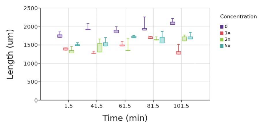
Figure 4. Diameter of beads at 20-minute increments in the presence of 0, 1x, 2x, and 5x the standard concentration of alginate lyase. Box and whiskers plot shows the median value (line), interquartile range (box), and the extent of the data (whiskers above and below at min/max data points) for three replicants at each concentration Image by author.
All beads exposed to 1x, 2x, and 5x alginate lyase were measured to have a slightly increasing diameter as well, with 1x alginate lyase increasing the least. Again, the increase was also likely due to saline intake After an hour, the beads in every solution looked relatively the same (Figure 5).
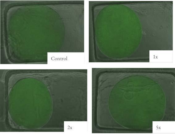
Figure 5. Images of beads under EVOS-Auto-fl-2 microscope imaging screen with GFP detection Top left: alginate bead exposed to 1x alginate lyase; top right: alginate bead exposed to 2x alginate lyase; bottom left: alginate bead exposed to 5x alginate lyase; bottom right alginate bead exposed to the control, saline. All images taken 61.5 minutes after the addition of the solution Image by author
The EDTA test ran for 17.5 minutes. Data on the diameter could no longer be measured after 17.5 minutes because the beads were fully dissolved, with no masses of microbeads seen in the images. The diameter of the control with saline remained relatively constant, only fluctuating slightly, likely due to saline intake (Figure 6). All beads exposed to 0.1 M, 0.15 M, and 0.2 M EDTA were fully dissolved by 17 5 minutes, with only a diffuse spread of microbeads remaining where the alginate beads were originally placed Beads exposed to 0 2 M had the smallest area of bright green, which is where the highest concentration of microbeads was. 0.1 M had the largest area of bright green for all of the microbeads pictured (Figure 7).
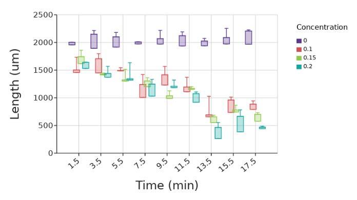
Figure 6. Diameter of beads at 2-minute intervals in the presence of 0 1, 0 15, and 0 2 M concentrations of EDTA The box and whiskers plot shows the median value (line), interquartile range (box), and the extent of the data (whiskers above and below at min/max data points) for three replicants at each concentration. Image by author.
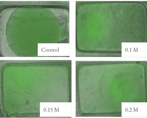
Figure 7. Images of beads under EVOS-Auto-fl-2 microscope imaging screen with GFP detection Top left: alginate bead exposed to 0 2 M EDTA; top right: alginate bead exposed to 0.15 M EDTA; bottom left: alginate bead exposed to 0.1 M EDTA; bottom right: alginate bead exposed to the control, saline All images were taken 17 5 minutes after the addition of the solution Image by author
The Emboclear (a combination of alginate lyase and EDTA) test ran for 46 5 minutes Data on the diameter could no longer be measured after 31 5 minutes because the beads were fully dissolved (Figure 8) The images of the Emboclear test were taken under the DAPI setting of the EVOS-fl-auto-2 Since no microbeads were present and the GFP setting was not used.
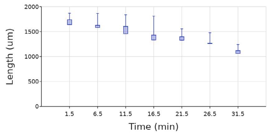
Figure 8. Diameter of beads at 5-minute intervals in the presence of Emboclear created using published procedures (Barnett & Gailloud, 2011). The box and whiskers plot show the median value (line), interquartile range (box), and the extent of the data (whiskers above and below at min/max data points) for three replicants at each concentration Image by author
The cell-free fiber test was performed using 0.1 M, 0 05 M, and 0 025 M EDTA The fibers were placed into a 96-well plate and imaged under the DAPI setting of the EVOS-fl-auto-2. All fibers exposed to 0 1 M were no longer visible within 1.5 minutes of the test initiation, which was before the first imaging scan had time to capture images Fiber exposed to 0 05 M EDTA and 0.025 M EDTA were no longer visible within 3.5 minutes of the test initiation (Figure 9).
The goal of this project was to determine the most effective way to dissolve alginate from around ASMCFs. Varying concentrations of alginate lyase and EDTA, both individually and in combination (Emboclear), were tested on alginate gel beads to determine which would dissolve the alginate the fastest without damaging the cells. EDTA at all concentrations tested was faster at dissolving alginate than the currently used concentration of alginate lyase 1x, 2x, and 5x the standard alginate lyase concentration used in the current ASMCF synthesis protocol had not fully dissolved the beads of alginate after 80 minutes, whereas 0.1 M EDTA fully dissolved the beads after five minutes
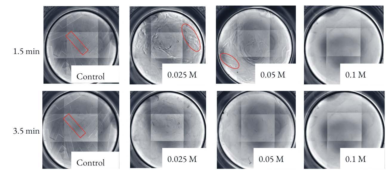
Figure 9. Images of beads under EVOS-Auto-fl-2 microscope imaging screen under the DAPI setting The top row depicts 12-well plates containing fibers exposed to (from left to right) 0 1 M, 0 05 M, 0 025 M, and the control, saline, at 1 5 minutes The bottom row depicts the same well plates at 3 5 minutes Image by author
More testing was done on fibers without cells using 0 1 M, 0 05 M, and 0 025 M EDTA The testing confirmed that EDTA dissolved the ASMCF faster than alginate lyase, with the 0.1 M concentration dissolving the fiber before 1 5 minutes, and the 0 05 M and 0 025 M dissolving the fiber in under 3.5 minutes. Based on the data reported here, a trial was run by another researcher on an ASMCF with live cells While the cells within the ASMCF remained alive when placed in EDTA at 0 05 M, the collagen inside the fiber was degraded, rendering this option unacceptable.
Emboclear, a commercial product that includes 0 5% w/v EDTA, and 0 2% w/v alginate lyase has been shown to work to dissolve alginate gel (Barnett & Gailloud, 2011). Emboclear is FDA-approved under a different name called “liquid embolic systems”. This is suitable for direct application to the human body and aids in the embolization of aneurysms If Emboclear is able to be used in the human body without harming it, this combination of EDTA and alginate lyase should likely be a safe option for the cells inside an environment created to emulate human muscle tissue, which is what the ASMCF does Concentrations of less than 1% w/v EDTA have been used in other situations
and shown to not degrade collagen (Gandolfi et al , 2018), so it is reasonable to expect that it would not dissolve the collagen inside the ASMCF. When Emboclear was recreated for these alginate bead experiments, it took 31 5 minutes for the beads to fully dissolve This was still faster than any level of alginate lyase tested on its own The next steps will be to test alginate lyase and EDTA on the fiber, and then try using it during the 3D printing process. These experiments will be pursued in the future
Determining the fastest method of dissolving the alginate while also keeping the smooth muscle cells inside the fiber alive is imperative to making sure the fiber works as well as possible while it is being used in 3D printers to make human tissue. This research represents an important step toward turning the possibility of 3D printing human organs into a reality.
This research project would not have been possible without the help of Dr Angela Panoskaltsis-Mortari, a Professor of Pediatrics at the University of Minnesota, and Kyleigh Pacello and Joe Broomhead, who are researchers at the 3D Bioprinting Facility at the University of Minnesota I am thankful for the help they
provided me in developing this project and carrying out experiments occurring in their facility With their assistance, I have learned skills in the realm of 3D bioprinting and biomedical engineering Also, I would like to thank Dr Kati Kragtorp for her support throughout my research, and for allowing me the opportunity to conduct laboratory research through Breck’s Advanced Science Research Program.
6 Quick Facts About Organ Donation (n d )
Abka-khajouei, R , Tounsi, L , Shahabi, N , Patel, A K , Abdelkafi, S , & Michaud, P (2022) Structures, Properties and Applications of Alginates Marine Drugs, 20(6), 364 https://doi.org/10.3390/md20060364
Barnett, B P , & Gailloud, P (2011) Assessment of EmboGel A Selectively Dissolvable Radiopaque Hydrogel for Embolic Applications Journal of Vascular and Interventional Radiology, 22(2), 203–211 https://doi org/10 1016/j jvir 2010 10 010
Gandolfi, M , Taddei, P , Pondrelli, A , Zamparini, F , Prati, C , & Spagnuolo, G. (2018). Demineralization, Collagen Modification and Remineralization Degree of Human Dentin after EDTA and Citric Acid Treatments Materials, 12(1), 25 https://doi org/10 3390/ma12010025
Gungor-Ozkerim, P S , Inci, I , Zhang, Y S , Khademhosseini, A , & Dokmeci, M R (2018) Bioinks for 3D bioprinting: An overview Biomaterials Science, 6(5), 915–946 https://doi org/10 1039/C7BM00765E
Hafen, B B , & Burns, B (2023) Physiology, Smooth Muscle In StatPearls StatPearls Publishing http://www ncbi nlm nih gov/books/NBK526125/
Kahrilas, P J (1997) ANATOMY AND PHYSIOLOGY OF THE GASTROESOPHAGEAL JUNCTION Gastroenterology Clinics of North America, 26(3), 467–486 https://doi.org/10.1016/S0889-8553(05)70307-1
Learn how organ allocation works OPTN (n d ) Retrieved December 22, 2023, from https://optn transplant hrsa gov/patients/about-transplantation/howorgan-allocation-works/
Mittal, R K (2011) Neuromuscular Anatomy of Esophagus and Lower Esophageal Sphincter In Motor Function of the Pharynx, Esophagus, and its Sphincters. Morgan & Claypool Life Sciences. https://www ncbi nlm nih gov/books/NBK54272/
New Technique Turns Alginate Solution Into Micron-Scale Gel Patterns Using Light (n d ) Retrieved January 11, 2024, from https://chbe umd edu/news/story/new-technique-turns-alginate-solu tion-into-micronscale-gel-patterns-using-light
Pushparaj, K., Balasubramanian, B., Pappuswamy, M., Anand Arumugam, V , Durairaj, K , Liu, W -C , Meyyazhagan, A , & Park, S (2023) Out of Box Thinking to Tangible Science: A Benchmark History of 3D Bio-Printing in Regenerative Medicine
and Tissues Engineering Life, 13(4), 954 https://doi.org/10.3390/life13040954
Schubert, J , Khosrawipour, T , Pigazzi, A , Kulas, J , Bania, J , Migdal, P , Arafkas, M , & Khosrawipour, V (2020) Evaluation of Cell-detaching Effect of EDTA in Combination with Oxaliplatin for a Possible Application in HIPEC After Cytoreductive Surgery: A Preliminary in-vitro Study Current Pharmaceutical Design, 25(45), 4813–4819 https://doi.org/10.2174/1381612825666191106153623
Vogt, C D , & Panoskaltsis-Mortari, A (2020) Tissue Engineering of the Gastroesophageal Junction Journal of Tissue Engineering and Regenerative Medicine, 14(6), 855–868 https://doi org/10 1002/term 3045
Zhu, B , & Yin, H (2015) Alginate lyase: Review of major sources and classification, properties, structure-function analysis and applications. Bioengineered, 6(3), 125–131. https://doi org/10 1080/21655979 2015 1030543
Noah Getnick and Evan Johnstone
Noah Getnick and Evan Johnstone
Introduction
Riding a bike is both a carbon-efficient mode of transportation and a great way to maintain fitness (Eisenman et al., 2010). However, the inherent difference in speed and size between cars and bikes makes it dangerous for cyclists to share the roads with cars, discouraging people from engaging in this beneficial activity (Reynolds et al , 2009) In the United States, there are approximately 49,000 automobilecyclist collisions a year, over 700 of which are fatal Riding a bike along busy streets can be an extremely difficult task. Cyclists must maintain visual awareness along the path of travel, while simultaneously glancing backwards at potential threats from the rear. Unsurprisingly, about 40% of car-bicycle collisions involve crashes where the car approaches the cyclist from the rear (Woongsun Jeon & Rajamani, 2016).
Technology dedicated to warning cyclists of approaching cars is still in its infancy The most common method of detection is through small radar systems attached to the rear of a bicycle. These systems include the Garmin Varia (Garmin, n d ), the Bryton Gardia (Bryton Gardia R300L, n.d.), and the Magene L508 (L508 Radar Tail Light, n d ) These systems have detection ranges of over 100 meters (Garmin, n.d.). However, in urban environments and crowded spaces, they often give false warnings, as the radar has no way to determine if a target is a motor vehicle or a harmless object (Garmin Varia Bike Radar - Worth It?, n d ) This shortcoming significantly limits the efficacy of these systems, since after several false alarms, cyclists may simply ignore subsequent warnings
Experimental solutions to warn bikers of approaching cars have been proposed using various sensing technologies Woongsun Jeon &

Rajamani designed a custom built sonar sensor system with a unique one-transmitter/tworeceiver design, paired with a single beam laser sensor for detection behind the bicycle. This system is effective at detecting vehicle position and orientation, but due to its single-beam sensor design, it has no way of visually confirming the identity of the detected object (Woongsun Jeon & Rajamani, 2016) Smaldone et al created an attached camera system to track oncoming vehicles This system uses a simple camera with a computer vision system to paint a “danger zone” within the camera frame, warning the cyclist when a car is detected in the zone However, the use of camera tracking puts a heavy workload on the processor, requiring an expensive PC mounted to the bike (Smaldone et al , 2011) Furthermore, neither of these examples are currently commercially available.
We designed a system that will detect a dangerous approach by an automobile from the rear and left side of a bicycle and provide an early warning to the cyclist. We used a sensor fusion system, consisting of a distance sensor coupled with a camera that uses computer vision to track oncoming vehicles. A TFLite object detection model (TensorFlow Lite, n d ) was trained and used to detect cars with the camera. The whole system was programmed with the Raspberry Pi 4 Model B single board computer (Raspberry Pi, n.d.-b, p. 4). The system is mounted on a rear bike rack.
The central unit and processor for our system is a Raspberry Pi 4B (2GB of RAM; Raspberry Pi, n d -c), a small computer designed for a variety of applications. We installed the Raspberry Pi
into a commercially available case (Raspberry Pi, n d -a) The Raspberry Pi has 40 GPIO (General Purpose Input/Output) pins for powering and communicating with sensors, servos, and lights, as well as a ribbon cable port for a camera
To program the Raspberry Pi, we plugged the computer into a monitor, mouse, and keyboard, allowing us to use the Raspbian operating system to run multiple applications. The Raspberry Pi is powered by a UPSPack power supply (Raspberry Pi UPSPack, n d ), which converts 3.7V from a 10000 mAh battery to 5V. The battery can supply power to the Raspberry Pi for at least two hours During preliminary testing, the Raspberry Pi ’s central processing unit (CPU) overheated frequently, causing temporary shutdowns, so we installed a Raspberry Pi case fan (Raspberry Pi, n.d.-d), designed to fit into the case. We used the Raspberry Pi configuration menu to run the fan automatically when the central processing unit temperature reached 60°C.
A Raspberry Pi Camera Model 2 (Raspberry Pi, n.d.-c) was used to capture video to be analyzed by an object detection model It attaches to the Raspberry Pi with a proprietary ribbon cable.
We used a distance sensor to detect nearby objects to complement the camera. Initially, we used a TFMini-S Micro LiDAR sensor (TFMini-S, n d ), which communicated with the Raspberry Pi through the UART serial port. However, this range decreased in outdoor conditions, since the sunlight interfered with the infrared waves it was transmitting. As a result, we switched to an ultrasonic sensor, which is unaffected by lighting conditions, since it uses sound waves to determine its distance from an object. We used a MaxBotix MB1010 sensor (MB1010 LV-MaxSonar-EZ1, n d ) It sends out sound waves to determine the range of an object by recording the time it takes for the wave to return to the receiver The sensor then sends out a digital pulse to the Raspberry Pi. Using code
from a Github repository (LV-EZ1 for Raspberry Pi, n d ), we wrote a script to convert the length of the pulse to distance measurements
To create a mount for the sensors, a 0.5 inch thick piece of Delrin plastic was cut, using a vertical bandsaw, to create a 3in x 3.5in rectangle with a rectangular (0.5in x 0.5in) cutout on the bottom right corner, to leave room for other components. The cut piece was secured to a servo motor (SunFounder Digital Servo, n d ) using the motor’s included plastic rotor mounts and bolts. Both sensors were mounted using 4-40 bolts
Initially, both sensors were mounted on the same face and plane, but to improve sensor accuracy, the ultrasonic sensor was later mounted at an angle This made it easier for the bicycle to detect cars passing to the side of the bicycle. A vertical bandsaw was used to cut a corner of the Delrin block to create a 45 degree slanted mount surface for the ultrasonic sensor.
To track cars with the camera, we developed an AI machine learning model using the TensorFlow Lite framework (TensorFlow Lite, n d ) It analyzes individual frames of a continuous stream of video to identify which objects in the frame are “cars'' and what their relative position is by drawing bounding boxes around them. We used a mobilenet-SSD model that we created using a publicly available Google Colab Notebook (Juras, n d ) To create the training data, we wrote a short script instructing the camera on the Raspberry Pi to take pictures every three seconds We then took pictures with the camera around a large parking lot, along a suburban county road, and in a business district We prioritized taking pictures of as many different types of cars as possible at varying angles, distances, and lighting. We took 928 photos in total After this, we labeled the images using LabelImg (Lin, n.d.; Figure 1). The LabelImg software created an XML file for each photo, representing the position of the cars
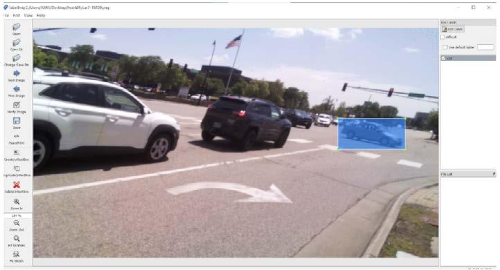
Figure 1. Representative image from LabelImg software. The blue highlighted box is the manually created bounding box for the car in frame. The data from each frame is converted into its own XML file. Figure by authors.
We used the Colab notebook to train our machine learning model with 80% of the images in our dataset. The model was verified on a separate 10% of our dataset to determine the accuracy of the model. We then quantized the model to allow it to run more efficiently on the Raspberry Pi, converting the 32 bit floating point values into 8 bit integer values. Quantizing the model, by definition, reduced the accuracy of the model, due to the 32 bit floating point values the model used being turned into 8 bit integer values. However, it also reduced the model to around a fourth of its original size and granted much lower strain on the CPU of the Raspberry Pi. The new model was deployed to the Raspberry Pi as a folder and used in place of the sample model.
Using the OpenCV Library, we wrote code to create a digital zone in each individual frame recorded by the camera This zone was rectangular, took up the entire left third of the screen, and was designated the “Danger Zone” (Figure 2) Using OpenCV, we tracked the center of each detected object and determined whether it lay within the Danger Zone We also filtered each object detected to make sure it was actually a car, by excluding objects that were wider than 800 pixels or taller than 600 pixels (the resolution of the camera images was 1280x720) This reduced incidents of the model incorrectly identifying entire swaths of the road as cars
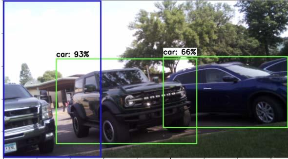
Figure 2. Danger Zone display. The purple rectangle defines the “Danger Zone,” which is displayed on the Raspberry Pi desktop Each detected car has the model ’s confidence level that the detected object is a car displayed above the green bounding boxes Figure by authors
When running the new model, the Raspberry Pi had a relatively low frame refresh rate of 1-2 frames per second To address this, we installed a Google Coral USB Accelerator (Coral, n.d.) to improve the performance of our model when running This device plugged into the Raspberry Pi through a USB connection and served as an additional processor for sensor data. The TFLite model is designed to be used with the Coral, so, other than a single command in the terminal, no additional code is needed.
Warning System
We initially modeled the warning system’s case in Fusion 360. Our design was a hollow case (Figure 3), made up of separate top and bottom pieces for easy access to wires. The case is in the shape of a box and is 2.5in x 5.5in and 1.5in tall. We added holes into the top to store three LED lights (red, orange, and green) and a slot on the side to access wires. We used a CNC router to cut the part out of a 2in x 4in piece of wood We used epoxy to secure the lights in the top of the case and soldered wires to them. The wires then connected to WAGO lever-nut connectors (Wire/Splicing Connectors, n.d.), which allowed for the easy securing and removal of wires that connect to the Raspberry Pi
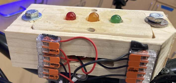
Figure 3. Warning system. Orange pieces are WAGO lever-nut connectors which are used to organize wiring for the LEDs. All electronics are contained within a wooden case. Figure by authors.
We used a commercially available rear bike rack (Lixada Rear Bike Rack, n d ) to serve as the main mount for our electronics. The rack attaches to the bicycle using a clamp-style mount (Figure 4) We used VHB tape (3M VHB Tape, n.d.) to secure the Raspberry Pi and the Google Coral to the rack. To mount the battery and power supply, we created a 3in x 5in x 1.25in “shelf” out of a polycarbonate sheet, which allows us to stack the two items securely (Figure 4) We also used VHB tape to secure this mount. We mounted the servo to the plate by cutting a hole at the back of the rack with a manual mill and bolting a servo mount bracket to the rack. The bike rack with electronics attached is mounted to the bike through a clamp that came with the bike rack
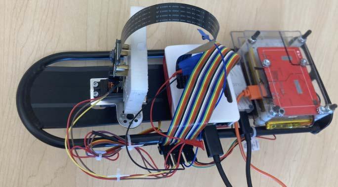
Programming
We used the Python programming language to program our system The Python Multiprocessing library (Multiprocessing, n d ) was far more efficient than this approach. The
multiprocess library creates separate processes that can be run at the same time within a file We implemented this to consolidate our distance sensor, computer vision, servo, and warning system code into one large Python file This also allowed us to use sensor values to control the servo and warning system.
We tested our system by mounting the rear bike rack and warning system to an adult-sized bicycle. We ran preliminary testing along the side of a minor, arterial, two-lane suburban county road in a residential area. We held the bike stationary in the bike lane while cars went by, simulating cycling in the bike lane We largely used this form of testing to verify the functionality of the object detection model and the ultrasonic sensor, so no data is included from these tests.
We turned on the orange light when the camera detected a car in the danger zone The red light was turned on when the ultrasonic sensor detected a target within five meters, for several consecutive measurements Initially, we set the system to turn on the red light if five readings under five meters are received in a row. During preliminary testing, the ultrasonic sensor consistently failed to detect cars for five consecutive readings. To amend this, we changed this ‘consecutive threshold’ to two consecutive readings required for the red light to turn on.
We ran moving tests (Mobile Testing) in an empty parking lot Either our research mentor or a team member would drive a car at approximately 10-15 miles per hour, while a member rode the bicycle at around 5 miles per hour. The car would slowly overtake the bicycle while it was in motion, testing what happens when the bicycle and car are both moving We kept the direction of testing the same between each trial During each round of testing, we checked for false positives by biking around the empty parking lot without the testing car present
Initial mobile camera testing was run in an open parking lot For this set of tests, the original camera mount was used, which kept the camera and ultrasonic sensor at the same angle. The sensors were angled slightly to the left of the bike since bikes typically are ridden on the right side of the road in the US. We tested with two different cars: a light gray Chevrolet Bolt and a dark gray Volkswagen Tiguan.
Out of a total of 30 trials, the camera detected the car 27 times (Table 1) The camera only missed detecting the car three times, likely due to the car being out of the camera’s frame. As long as the front of the car was in view of the camera, it accurately detected the two cars Moreover, the warnings were given extremely early, with the car being detected by the system well before it could be heard by the cyclist, even in an empty parking lot. When we biked around the parking lot without the testing car, the camera did not return any false positive warnings of the empty parking lot.
Table 1. Mobile Testing 1. Warning LED results from mobile testing of sensors. Green (No warning), Orange (camera warning), Red (ultrasonic warning).
We focused the second round of mobile tests on getting consistent ultrasonic sensor warnings We did not use the camera for these tests We used the updated sensor mount for this test, which angled the ultrasonic sensor 45 degrees to the left of the bike, to increase the likelihood of detecting passing cars. We also reduced the consecutive threshold to two consecutive measurements of five meters or less Since the ultrasonic sensor only detects distance, we only tested with a Volkswagen Tiguan
We organized the sensor readings into four groups: Off (no warnings), intermittent flashing (a few short flashes by the light), constant flashing (either a few long flashes or many short flashes), and on (a significant period of the light being on with no flashing). With the increased angle and reduced threshold for warning, the ultrasonic sensor returned some form of warning in every test. Although it never was consistently on, the warning system flashed intermittently 4 times and flashed continuously 11 times, out of 15 total trials. The warning light began flashing when the car was about a car’s length behind the bike, and ended just as the car was passing the bicycle. This gave the testing biker a significant period of time to notice the passing car before it went by. As in the camera tests, there were no false positives from the ultrasonic sensor warning when the bike was ridden in the parking lot without the testing car.
The primary issue with the camera was that the orange light would occasionally freeze for 10-15 seconds, remaining illuminated even when the camera was blocked, making it impossible for any cars to be detected. This indicated that the object detection process was overloaded with data
In addition, the ultrasonic sensor failed to detect the car in all trials. Although the ultrasonic sensor can detect objects slightly to the side, passing cars were too far to the side to be in the detection cone. In addition, the consecutive threshold of five probably reduced the likelihood of receiving a warning
To perform the combined sensor tests, we used the modified sensor mount, which angled the ultrasonic sensor approximately 45 degrees to the left of the camera We recorded LED warnings given by the system for each trial. The consecutive threshold for the ultrasonic sensor remained at two consecutive frames We tested with a dark gray Volkswagen Tiguan.
In all 15 trials, the ultrasonic sensor successfully detected the car at a range of around 1 meter Out of the 15 trials, the camera gave a warning 14 times, with only one test returning no camera warning when the car was behind the bike
No false positives occurred when biking in the empty parking lot Code freezing occurred three times during the entire testing period when the camera would record a warning, but the warning would not turn off for 15-30 seconds, even when a hand was placed to block the camera
Inconsistent lighting was also an issue for our system. The testing was conducted about an hour before sunset, during autumn in Minnesota, and the sun would often point directly into the camera during testing. When returning from the finish point of each trial to the start point, the camera failed to detect the car from other angles. This was likely due to the lack of lighting contrast in low light In contrast, when the camera was pointed in the general direction of the sun it interfered with the object detection algorithm, causing the camera to be effectively blinded and unable to show any frames with usable data (eg. cars) to the machine learning system Despite these inaccuracies, the overall success of these tests demonstrated a proof of concept for our system. When all sensors were put together, our system provided an accurate and timely warning to cyclists of approaching cars under daytime conditions about 93.3% of the time
The current code running on the system is fully contained within one file The system is set up by running several commands to initiate the object detection model and servo before running the main file The Python script continuously runs until a user interrupts.
During normal operations, when no warnings are detected, the warning system returns a green light When the camera detects a car in the danger zone, an orange light is returned. When the ultrasonic sensor detects an object within five meters for two consecutive frames, a red light is returned. This serves as a last-minute warning, giving the cyclist an alert a few seconds before the car passes Typically, the camera detects the car within a distance of 75 meters from the bicycle, sending an orange warning, but as the car gets to within 5 meters, the camera
loses detection because the car becomes too large within the camera’s frame At this point, the ultrasonic sensor sends a red warning, indicating that the car is about to pass the bicycle These warnings combine to produce a two-level system that alerts bikers when a car is approaching and passing the bike.
When the system is running, the battery can power the Raspberry Pi for 1-2 hours During testing, detection accuracy remained stable for periods of about an hour, but decreased after longer periods of time
The total cost of the current system is estimated at $240 more expensive than the $150 cost of the radar-only model of the Garmin Varia (Garmin, n.d.). The primary component in this price is the use of the object detection system, since it requires the use of the camera and Google Coral. However, the total cost of the system was inflated by retail prices, which are much higher than would be expected if the system was to be manufactured, like the Garmin Varia
During testing, the Raspberry Pi would occasionally freeze, preventing warning lights from changing state. It would unfreeze after a period of about 30 seconds to a minute. This error was likely due to the limitations of the Raspberry Pi ’s processing power or to overheating slowing processing speeds. When the camera moved around or turned rapidly, the rapidly changing images exceeded the Raspberry Pi's processing power. This caused the system code to run slowly or even freeze, affecting when and how the warning lights came on or off. In addition, when pointed into the sun, it was nearly impossible for the camera to detect cars After the completion of this prototype, the Raspberry Pi 5 was released, with significant improvements to performance and random access memory (RAM). Using this model would allow the Raspberry Pi to smoothly process images, even when faced with bright or rapidly changing lighting conditions (Raspberry Pi,
n.d.-e, p. 5). The Raspberry Pi 5 (4GB RAM version) is more expensive, at $60, compared to $45 for the Raspberry Pi 4B (2GB RAM version) we used, but the improvement in performance would far outweigh the increase in cost
Another possible modification to broaden the capabilities of this system would be to install a longer range distance sensor Although the camera could detect cars accurately from up to around 76 meters away, it could not determine the distance to the car, so the ultrasonic sensor was the only way to quantify how far away the car was. The MB1010 ultrasonic sensor we used has a range of about 6 5 meters, which allowed us to effectively give a warning when the car was about to pass the bicycle. A longer range LiDAR, RADAR, or ultrasonic sensor would allow us to calculate the relative velocity of the car. With a longer range, calculations for relative velocity would become more reliable, as there would be more total measurements. In this way, ultrasonic sensor warnings could be given based on the estimated time for the car to pass the cyclist, meaning that timely warnings could be delivered for both slow and fast moving cars. However, this change in distance sensors would come with a significant increase in cost, as there are few commercially available long range distance sensors
The system was not trained to be used at night, sundown, or sunup, so retraining the model with additional photos of cars at night, and during sunset and sunrise, would allow for the system to be used in more situations. Additional improvements to the object detection would be training the system on more training steps with a larger and more diverse dataset, such as motorcycles, trucks, and buses It would also help to train the object detection model with additional photos, especially in different weather and lighting conditions In particular, adding training data to detect vehicles at dusk and at night would be helpful, especially since car headlights provide a clear marker to detect These modifications would improve not only
accuracy, but the circumstances in which our system is useful
Another improvement would be to enhance the warning system for the cyclist. The current system of a wood case with LED lights was a temporary design to allow for the easy transmission of warnings from the Raspberry Pi. By connecting via Bluetooth between a Raspberry Pi and a cell phone, an app on the phone could be used as a warning system. Using a phone would allow for adjustments in brightness at night and during the day, so warnings would be easier to see. Commercially available phone mounts would also be more secure than the current 3D printed clips During testing, warnings sometimes flashed on and off frequently, especially with the ultrasonic sensor, so code could also be added to “smooth” out the warnings by keeping the warning lights on for 0.25 seconds after a warning was received.
Ultimately, an important next step in prototype development will be to provide weather and shock protection for the system. Adding a protective cover over the top and front of the mount would protect the electronics from any precipitation, without occluding the camera and ultrasonic sensor The best way to protect the sensor system would be to construct a purpose-built electronics case that would securely store electronics inside a 3D-printed box. Sensors could be protected by still placing them into the case, but fitting the camera lens and ultrasonic sensor transmitter/ receiver into small holes in the case.
Our system can significantly improve bicycle safety by delivering accurate warnings to bikers, allowing them to avoid cars. The long range of the camera detection algorithm is especially useful on major roads, where it can accurately detect fast moving cars well in advance of the car passing the bike In busy, urban environments, the camera can distinguish between random objects and cars, a major improvement over current bike detection systems When available publicly, this system
will make biking a safer experience, encouraging more people to try this healthy and environmentally friendly activity
We would like to express our profound gratitude to Dr Kati Kragtorp for her constant guidance throughout our project Her support was critical in helping us to refine our ideas, plan future steps, and present and write about our work Thank you to Breck School for providing project resources.
3M VHB Tape (US) (n d ) Retrieved August 22, 2023, from https://www 3m com/3M/en US/vhb-tapes-us/
Bryton Gardia R300L (n d ) Bryton USA Online Shop Retrieved September 14, 2023, from https://us eshop brytonsport com/products/gardia-r300l
Coral (n d ) Coral Retrieved September 8, 2023, from https://coral ai/
Eisenman, S B , Miluzzo, E , Lane, N D , Peterson, R A , Ahn, G -S , & Campbell, A T (2010) BikeNet: A mobile sensing system for cyclist experience mapping ACM Transactions on Sensor Networks, 6(1), 6:1-6:39 https://doi.org/10.1145/1653760.1653766
Garmin (n d ) Garmin VariaTM RTL515 | Bike Radar and Tail Light Garmin Retrieved August 4, 2023, from https://www garmin com/en-US/p/698001
Garmin Varia bike radar (n d ) Retrieved August 4, 2023, from https://www youtube com/watch?v=STPw1QPLn2s
GPIO Ribbon Extension Cable. (n.d.). Micro Center. Retrieved August 30, 2023, from https://www microcenter com/product/450152/qvs-8-gpio-ribbon-e xtension-cable-for-raspberry-pi-a-b-(26-pins)
Juras, E (n d ) TensorFlow Lite Object Detection API in Colab Retrieved August 30, 2023, from https://colab research google com/github/EdjeElectronics/TensorFl ow-Lite-Object-Detection-on-Android-and-Raspberry-Pi/blob/mast er/Train TFLite2 Object Detction Model ipynb
L508 Radar Tail Light (n d ) Retrieved September 14, 2023, from https://www magene com/product l508 html
Lin, T (n d ) labelImg: LabelImg is a graphical image annotation tool and label object bounding boxes in images [Python] Retrieved September 8, 2023, from https://github com/tzutalin/labelImg
Lixada Rear Bike Rack (n d ) Retrieved June 23, 2023, from https://www amazon com/Lixada-Bicycle-Retractable-Aluminum-I nstall/dp/B07TYVV531/ref=sr 1 3?crid=789E15VTD186
LV-EZ1 for Raspberry Pi (n d ) Retrieved August 22, 2023, from https://github com/hatobus/LV EZ1 for raspi
MB1010 LV-MaxSonar-EZ1 (n d ) MaxBotix Retrieved August 22, 2023, from https://maxbotix.com/products/mb1010
Multiprocessing (n d ) Python Documentation Retrieved September 6, 2023, from https://docs python org/3/library/multiprocessing html
Raspberry Pi (n d -a) Buy a Raspberry Pi 4 Case Raspberry Pi Retrieved August 23, 2023, from https://www raspberrypi com/products/raspberry-pi-4-case/
Raspberry Pi (n d -b) Buy a Raspberry Pi 4 Model B Raspberry Pi Retrieved August 23, 2023, from https://www raspberrypi com/products/raspberry-pi-4-model-b/
Raspberry Pi (n d -c) Buy a Raspberry Pi Camera Module 2 Raspberry Pi Retrieved May 26, 2023, from https://www raspberrypi com/products/camera-module-v2/
Raspberry Pi (n d -d) Raspberry Pi 4 Case Fan Raspberry Pi Retrieved August 23, 2023, from https://www raspberrypi com/products/raspberry-pi-4-case-fan/
Raspberry Pi (n d -e) Raspberry Pi 5 Raspberry Pi Retrieved November 1, 2023, from https://www raspberrypi com/products/raspberry-pi-5/
Raspberry Pi UPSPack. (n.d.). MakerFocus. Retrieved May 26, 2023, from https://www makerfocus com/products/raspberry-pi-expansion-boa rd-ups-pack-standard-power-supply
Reynolds, C C , Harris, M A , Teschke, K , Cripton, P A , & Winters, M (2009) The impact of transportation infrastructure on bicycling injuries and crashes: A review of the literature Environmental Health, 8(1), 47. https://doi org/10 1186/1476-069X-8-47
Smaldone, S , Tonde, C , Ananthanarayanan, V K , Elgammal, A , & Iftode, L (2011) The cyber-physical bike: A step towards safer green transportation Proceedings of the 12th Workshop on Mobile Computing Systems and Applications, 56–61 https://doi org/10 1145/2184489 2184502
SunFounder Digital Servo. (n.d.). Retrieved May 26, 2023, from https://www amazon com/SunFounder-Digital-Helicopter-Fix-Win g-Airplane/dp/B01KZKOIZC/ref=sr 1 18?crid=900RF263DSCM
TensorFlow Lite (n d ) TensorFlow Retrieved July 31, 2023, from https://www tensorflow org/lite
TFMini-S (n d ) Retrieved May 26, 2023, from https://www sparkfun com/products/16977
VNC Viewer (n d ) RealVNC® Retrieved August 23, 2023, from https://www realvnc com/en/connect/download/viewer/
Wire/Splicing Connectors (n d ) WAGO USA Retrieved August 22, 2023, from https://www wago com/us/discover-wire-and-splicing-connectors
Woongsun Jeon, & Rajamani, R. (2016). A novel collision avoidance system for bicycles 2016 American Control Conference (ACC), 3474–3479 https://doi org/10 1109/ACC 2016 7525451
Matthew Manacek and Samantha Dvorak
Matthew Manacek and Samantha Dvorak
Introduction
Alzheimer’s disease (AD) is a neurodegenerative disease that slowly destroys brain function and memory In the United States alone, Alzheimer’s affects more than six million people, a number that is expected to rise to nearly 13 million by 2050 (Alzheimer’s Disease Facts and Figures, n.d.). It is the most common form of dementia for a person to be diagnosed with, starting as mild memory loss and progressing into mood swings, forgetting loved ones, and difficulty breathing and swallowing. Individuals with Alzheimer’s eventually lose total autonomy, requiring constant care and help performing daily activities.
In 1906, Dr Alois Alzheimer noticed changes in the brain tissue of a woman who had died of an unusual mental illness. Her symptoms included memory loss, language problems, and unpredictable behavior. After she died, he examined her brain and found many abnormal clumps now called amyloid plaques and tangled bundles of fibers now called neurofibrillary, or tau, tangles (Breijyeh & Karaman, 2020) Today, amyloid plaques and neurofibrillary tangles are still considered two major pathological hallmarks of the disease, but our understanding has extended far beyond Dr Alzheimer’s initial discoveries.
Amyloid precursor protein (APP) is normally expressed in adult brain tissue While it is not fully understood, researchers speculate that it may help bind other proteins to neurons and other cells The cleavage of APP can occur at different points in the molecule by the enzymes beta-secretase, alpha-secretase, or gammasecretase, creating different forms that have

varying impacts on the brain (Asai et al , 2003; Vassar et al., 1999; Wolfe, 2008). APP is cleaved by beta-secretase and gamma-secretase to yield amyloid-beta peptide (Aβ) Excessive Aβ can assemble into fibrillar structures that form microscopically visible plaques or aggregate into soluble oligomers in the brain parenchyma (Ashe, 2020). Aβ oligomers are believed to be the most toxic as they can freely disperse throughout the brain and interfere with normal brain function (Westerman et al., 2002).
Fibrillar structures are also harmful to the brain but tend to develop only in later stages due to the massive accumulation of Aβ (Zempel et al., 2010). Before fibrillar structures have formed, Aβ oligomers have already damaged neurons Because this damage has occurred from the dispersion of Aβ, when plaques are removed from Alzheimer’s patients in the later stages of the disease, the improvement in memory and overall brain function is marginal and temporary.
Due to damage from Aβ occurring before fibrillar structures have assembled, Aβ₁ ₄₂ oligomers are currently being studied to understand their various impacts on the brain (Bernabeu-Zornoza et al., 2021). Aβ₁ ₄₂ oligomers are understood to be a key form of Aβ that induces toxic effects As Aβ oligomers disperse throughout the brain, they interact with receptors in the dendritic spines of the neurons, such as glutamate receptors N-methyl-Daspartate (NMDAR) and alpha-amino-3hydroxy-5-methyl-4-isoxazolepropionic acid (AMPAR; Zhang et al , 2022) Their interaction causes these receptors to be overstimulated, leading to NMDAR and AMPAR internalization, via an influx of calcium into the cell (Zhang et al., 2022). This calcium influx overactivates the
calmodulin-dependent protein kinase II (CAMKKII) and the adenosine monophosphateactivated protein kinase (AMPK) pathway which leads to spine loss, another synaptotoxic effect of Aβ (Mairet-Coello et al , 2013) Additionally, CAMKII overactivation decreases long-term potentiation in neurons and destabilizes AMPARs, leading to synaptic loss (Zhang et al , 2022) Furthermore, the overexpression and accumulation of Aβ can cause mitochondrial dysfunction and disrupt the axonal transport of mitochondria, leading to synapse starvation and, eventually, neurodegeneration (Zhang et al., 2022) The Aβ oligomer Aβ*56 has a particularly devastating effect on cognitive function. It appears in brain tissue before the onset of behavioral deficits (Amar et al , 2017), and, as such, is a potential key target for Alzheimer’s treatment.
In addition to Aβ, the microtubule-associated protein tau undergoes changes during Alzheimer’s disease development. Under normal physiological conditions, tau stabilizes neuronal microtubules (Avila et al , 2004) In a disease-state, however, tau becomes hyperphosphorylated, detaches from the microtubules, and eventually accumulates in the dendritic spines (Breijyeh & Karaman, 2020). Tau accumulation and hyperphosphorylation cause cognitive and synaptic deficits, leading to neurodegeneration and memory loss. Tau is hyperphosphorylated on the KXGS motifs by several kinases, specifically CAMKII, Microtubule affinity-regulating kinase (MARK), and AMPK families (Amar et al., 2017). In order for tau to induce synaptic dysfunction and memory deficits seen in Alzheimer’s, it must be phosphorylated at one of the key sites including Ser262, Thr205, Th212, Thr217, and Thr231 (Lilek et al., 2023). Tau phosphorylation at sites Ser262 and Ser356, specifically, has been shown to mediate Aβ₁ ₄₂ oligomer-induced dendritic spine loss (Iijima et al., 2010).
During AD, tau can also be cleaved by caspases (Rissman et al , 2004) Particularly, caspase-2mediated human tau cleavage at aspartate-314 produces Δtau314 and induces cognitive
impairment and hippocampal degeneration in mouse models of dementia (Zhao et al , 2016) In addition, levels of Δtau314 are elevated in individuals with AD and multiple tau-related neurodegenerative disorders (Liu et al , 2019, 2020; Ossenkoppele et al , 2019) These findings indicate a broad impact of this cognitionaffecting event on a variety of diseases Further, an association between Δtau303, the mouse equivalent of human Δtau314, and cognitive impairment is established in a transgenic AD mouse model (Kemper et al , unpublished data) This leads Δtau303 to be a species of interest.
The interaction between Aβ and tau is not fully understood and depends on the type of Aβ present (Amar et al., 2017). Current research suggests that Aβ oligomers can activate a cascade of effects that cause tau hyperphosphorylation via several kinases, including the CAMKII-AMPK pathway. Additionally, tau has been shown to mediate the synaptotoxic effects of Aβ via Src family non-receptor tyrosine kinase Fyn (Briner et al., 2020). Tau facilitates Fyn diffusion into dendritic spines, which in turn enhances the activity of NMDARs (Zhang et al., 2022). Though tau can mediate its toxicity, Aβ is ultimately upstream of tau in Alzheimer’s pathogenesis. Because the toxic effects of Aβ and tau are closely related, a deeper understanding of the connection between various forms of Aβ and tau is needed for future drug development.
The mouse model Tg2576 overexpresses human APP with the “Swedish” mutation, which results in increased levels of secreted Aβ peptides in the central nervous system This contributes to age-induced elevated levels of all types of Aβ, and ultimately, the development of Aβ plaques (Hsiao et al , 1996) Levels of insoluble Aβ aggregates increase as the mice age, impacting their spatial memory (Westerman et al., 2002).
We looked specifically at Aβ*56 and Δtau303, two cognition-affecting entities in Tg2576 mice (Hsiao et al., 1996), an AD mouse model expressing human APP with the “Swedish” mutation We used immunoprecipitation and western blotting to measure levels of both
Aβ*56 and Δtau303 in brain tissue samples from mice aged 5 to 28 months The samples differed in age and sex; tissue samples from wild-type mice were used as a control. Our results showed that levels of Aβ*56 increase with age in Tg2576 transgenic mice However, we did not find a significant correlation between levels of Aβ*56 and Δtau303
Right hemispheres of Tg2576 and nontransgenic littermates at ages ranging from 4 to 27 months were previously collected by trained researchers and stored at 80°C. A number 1 to 36 was randomly assigned to these specimens for treatment blinding. Specimens were kept on dry ice for tissue quality preservation. The right forebrain from the rest of the tissue and added to chilled 5-mL Wheaton glass tubes containing 1 mL of ice-cold Tris-buffered saline extraction buffer The tissue specimens were homogenized, then transferred into 1.5-mL microcentrifuge tubes, and centrifuged for 90 minutes at 13,000 rpm at 4°C Resulting supernatants were stored at -20°C.
The brain extracts were thawed for 30 minutes at room temperature (RT), then centrifuged at 13,000 rpm at 4°C for 90 minutes, and supernatants were transferred to 1.5-mL microcentrifuge tubes 50μL of IPDB-washed Protein G Sepharose beads were added to the brain extracts of each mouse and nutated for 1 hr at 4°C, then centrifuged for 5 minutes at 10,000 rpm at 4°C The resulting supernatants were transferred to 1.5-mL microcentrifuge tubes and 50 μL of IPDB-washed Protein G Sepharose beads were added The steps including and following nutation were repeated, and the supernatants were labeled as the final product
A bicinchoninic acid (BCA) assay kit was used to determine the protein concentrations of the brain extracts The brain extracts and BCA standards were thawed at RT and pipetted into a 96-well plate The final volume of each well was
Matthew Manacek and Samantha Dvorak
250 μL of reagent plus 2.5 μL of the extract or standard There were duplicates of each extract and standard to control for pipetting errors The BCA standards were diluted to create 11 standards ranging from 8000 ug/ml to 0 ug/ml A plastic seal was added to the top of the plate to prevent spillage. Then, the plate was placed on a Bio-Rad orbital shaker for 10-20 seconds on level 7 The plate was then placed in the 37°C incubator for one hour. Afterward, the plate was removed from the incubator and sat at RT for 5 minutes The plastic seal was carefully removed and the plate was placed in the plate reader. The program on the plate reader was used to determine protein concentrations
Immunoprecipitation:Immunocomplex formation
Each brain extract with 1.2 mg total protein was placed in 1 5-mL microcentrifuge tubes and inhibitor-containing IP Dilution Buffer was added to bring the final volume to 0.5 mL. Then, antibodies [4 µL (~10 µg) of mouse monoclonal antibody 4F3 recognizing the C-terminus of Δtau303 when probing for Δtau303, 2 7 µL (~3 µg) of rabbit monoclonal antibody D8Q7I recognizing the C-terminus of Aβ(x-40) when probing for Aβ*56, or 2 µL of rabbit polyclonal antibody K9JA recognizing human tau amino acids 243-441 when probing for full-length tau] were added to each tube, followed by 50 µL of pre-washed Dynabeads Protein G slurry Tubes were nutated at 4°C for 12-18 hours.
The tubes containing immunocomplexes were briefly centrifuged, inserted into the magnetic microcentrifuge rack, and allowed to sit at RT for 1 minute. The supernatant was discarded. The beads were washed with IPDB twice more When 1 mL of IP Dilution Buffer (without inhibitors) was added, the Dynabeads Protein G matrix was fully resuspended
The tubes were removed from the nutator and centrifuged for 5 seconds at RT. The tubes were inserted into a magnetic microcentrifuge rack and sat at RT for 1 minute Each supernatant was transferred to a new, 1.5-mL, autoclave-sterilized microcentrifuge tube and stored at -20°C We added 1 mL of ice-cold Wash Buffer A to each
tube and fully resuspended the Dynabeads Protein G matrix Then, the tubes were nutated at 4°C for 5 minutes This process was repeated, using 1mL of ice-cold Wash Buffer B. The supernatant was discarded The pellet was kept
Immunoprecipitation: Elution
The pellet was resuspended by adding 25 μL of IgG Elution Buffer to each microcentrifuge tube. Proteins were eluted off the Dynabeads Protein G matrix by placing the tube on a shaker at 22°C, 1,250 rpm for 5 minutes. The tubes were then centrifuged at RT for 5 seconds Each tube was inserted into the magnetic microcentrifuge rack, and let sit at RT for 1 minute The supernatant containing the eluted proteins from each tube was transferred to a new tube. 1.25 µL of Neutralization Solution was immediately added to the 25 µL supernatant, mixed well, and stored on ice. This process was repeated twice, resulting in three 26 25 µL solutions for each sample Eluted materials were combined, resulting in a total volume of 78.75 µL for each sample Each sample was concentrated to 15-20 µL using a speed vacuum concentrator
Western Blot: Gel electrophoresis
We added 7 μl of 4X sample loading buffer to the concentrated eluted materials The mixture was boiled at 95°C at 1000 rpm for 5 minutes using a thermoshaker and then centrifuged at RT at 9,300 g for 5 minutes
The samples were loaded into 1.0 mm-thick, 10-well, Invitrogen™ Novex™ 10-20% Tricine Mini Protein Gels, along with 3 µL of the Precision Plus Protein Dual Color Standards ladder and either 10 ng of purified recombinant Δtau303 or 1 ng of Aβ1-40 Gels were run in 1X NOVEX Tricine SDS Running Buffer using an XCell SureLock Mini-Cell driven by a PowerPac™ HC Power Supply, at RT, under a constant voltage of 125 V for 90 minutes.
Western Blot: Protein transfer
To transfer the proteins, a 0 22-μm nitrocellulose membrane was cut into 9 cm by 7.5 cm sections. The filter paper and the pads were placed on either side of the membrane, with two pads on
the bottom and one in between gels. This gel-membrane assembly was placed into an XCell II™ Blot Module Then, the XCell Blot Module was placed into an XCell SureLock Mini-Cell and filled with 1X NuPAGE® Transfer Buffer, and the rest of the module with ddH2O. It was connected to a PowerPac™ HC Power Supply at a constant voltage of 25V for two hours before storing it at 4°C
Western Blot: Primary antibody
After the transfer, the nitrocellulose mem branes were removed and cut to only retain the area blotted with proteins. These were placed into an Extra Large (15 4 x 10 4 cm) PerfectWestern™ box containing 50 mL of 1X phosphate-buffered saline (PBS) with the side blotted with proteins facing downwards To improve protein detection, membranes were microwaved at a power level of 10 for 25 seconds, allowed to cool for 4 minutes, processed again for 15 seconds, and then allowed to cool at RT for another 4 minutes. The membrane was flipped upside down to allow the side blotted with proteins to face upwards and transferred to a Large (11.7 x 9.0 cm) PerfectWestern™ box containing 17 mL of Blocking Buffer at 25-30°C The membrane was blocked using an orbital shaker at RT at 69 rpm for 1 hr. Then, we added 3 4 μL of biotin-conjugated tau5 mouse monoclonal antibody for the detection of Δtau303 or 17 μL of biotin-conjugated 82E1 mouse monoclonal antibody for the detection of Aβ*56 to the box containing the membrane and blocking buffer. The membrane was incubated in the blocking buffer with the antibody by rotating at 69 rpm on the orbital shaker at 4°C for 14-16 hr.
Western Blot: Secondary Antibody and Image Capture
34 mL of TBST Wash Buffer was added to the box with the membrane. The membrane was rinsed by gently rotating the box by hand approximately 20 times The TBST Wash Buffer was discarded and the membrane was washed using 17 mL of TBST Wash Buffer and gently rotated at 79 rpm on an orbital shaker at RT for 5 minutes. The TBST Wash Buffer was discarded,
and this wash process was repeated three more times Next, we added 17 mL of TBST Wash buffer at RT and 3 4 μL of horseradish peroxidase (HRP)-conjugated NeutrAvidin to the box with the membrane and rotated at 69 rpm on an orbital shaker at RT for 30 minutes The rinse and wash process was repeated. Next, 5 mL of SuperSignal™ West Femto Max Sensitivity
Substrate A and 5 mL of SuperSignal™ West Femto Max Sensitivity Substrate B were added. The box was rotated at 200 rpm on an orbital shaker at RT for 5 minutes Then, the membrane was placed in a clear plastic loading sheet before it was revealed with a ChemiDoc MP Imaging System
Western blot images from the ChemiDoc MP Imaging System were imported into Bio-Rad’s Image Lab software. Aβ*56 and Δtau303 were quantified separately using the Volume tools on the software Aβ*56 was compared to Aβ monomers using volumetric tool analysis. The western blot image was imported into Bio-Rad’s Image Lab Software The image was then cropped to retain just the western blot and rotated as necessary so that the bands were straight Next, we identified the location of Aβ*56 at the 56kDa molecular weight and Aβ monomers ~4 5kDa molecular weight Then we used Bio-Rad’s volumetric tools to create a box around the largest band of Aβ*56. Eight copies of this band were created and placed at the 56 kDa mark The same was repeated for the monomers, at the ~4.5 kDa molecular weight. When quantifying the monomers, some of the biggest bands were so large that they spilled over into neighboring lanes, so the volumetric boxes had to be adjusted to avoid picking up a false signal This was done in such a way that all of the monomers were still included in each box. The synthetic Aβ1-40 was also quantified as a comparison between western blots by placing a box around its location at ~4.5 kDa molecular weight Next, Bio-Rad’s analysis table tool was used to determine the mean background, adjusted volume, and standard deviation of the samples To determine if a given signal was
Matthew Manacek and Samantha Dvorak
significantly greater than the background, we added 3x the standard deviation to the mean and compared this value against the adjusted volume of the sample. If the adjusted volume of the sample was greater, then the signal was said to be significantly above the background, and Aβ*56 was deemed detectable. The value of Aβ*56 was compared against the Aβ monomers present in each respective sample by dividing the adjusted volume of Aβ*56 by the adjusted volume of the monomers
Three types of bands were identified as Δtau303 (Kemper, Liu, and Ashe et al. unpublished data). This is likely due to them behind variations of Δtau303 originally from different tau isoforms and/or different post-translational modifications of tau proteins: a solid band at 37 kDa, a group of three thin bands directly above the 37 kDa mark, and a single thin band directly beneath the 37 kDa mark. All of these bands were measured for analysis
We used western blotting to measure the relative amounts of Aβ*56 and Δtau303 in five brain tissue samples collected from wild-type mice. These mice consisted of three females, aged 5 3 months, 16 7 months, and 25 7, and two males, aged 5.3 months and 16.7 months. All wild-type samples were negative for both Aβ*56 and Δtau303 Aβ*56 results of one female, aged 5 3 months, an d Δtau303 results of one male, aged 5 3 months, were excluded due to an artifact (smear) on the gel that obscured quantification
We used western blotting to measure the relative amounts of Aβ*56 and Δtau303 in 30 brain tissue samples collected from Tg2576 mice. These samples were collected over 22 years as part of other research Ages ranged from 5 3 months to 27.7 months and included both male and female mice (Table 1)
Table 1. Number of Tg2576 samples included in the analysis by gender and age range.
Gender Age range (months) 5.3 - 9.8 11.3 - 18 20.7 - 27.7 Total
Male 6 5 1 12
Female 7 7 4 18
Total 12 13 5 30
Presence of Δtau303 and Aβ*56
Of the 30 samples taken from Tg2576 mice, six did not show any significant Aβ*56 band intensity or Δtau303 band intensity. There were 21 samples ranging from 5.3 months to 27.7 months that showed significant Aβ*56 band intensity but no significant Δtau303 band intensity. Four samples from ages 5.3 months to 11 3 months showed a significant Δtau303 band intensity but no significant Aβ*56 band intensity. Five samples with ages ranging from 5.3 months to 27 6 months showed both significant Aβ*56 band intensity and a significant Δtau303 band intensity (Figure 1).
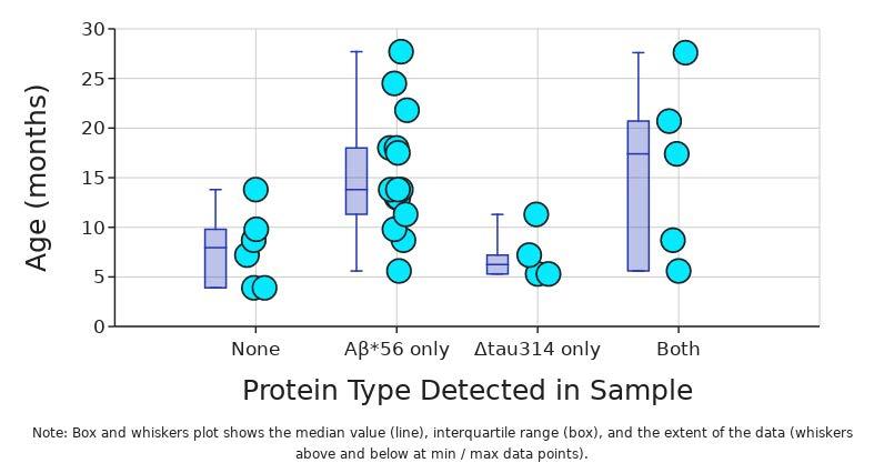
Figure 1. Type of protein (Aβ 56 or Δtau303) detected in male and female brain samples from Tg2576 mice (n = 30). Data points are offset for clarity. The box and whiskers plot represents the median value, interquartile range, and extent of the data above and below at the minimum and maximum points (Figure by authors)
Levels of Aβ*56
The intensities of Aβ*56 bands from each Tg2576 sample were calculated to determine the level of protein expression Levels of Aβ*56 had a positive, significant correlation with age (p < 0.05; Linear Regression; Figure 2).
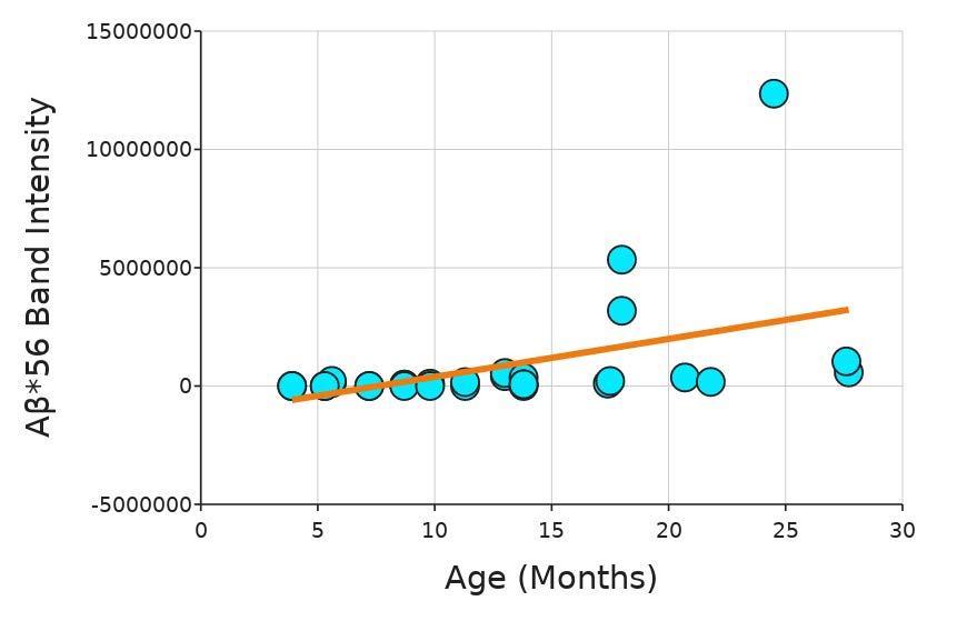
Figure 2. Age versus Aβ*56 band intensity in male and female brain samples from Tg2576 mice (n = 30; p < 0 05) Samples with intensities that were not significantly different from the background were set to zero for this analysis (Figure by authors)
Levels of Δtau303
The intensity of each sample’s Δtau303 bands and full-length tau band intensity were recorded Since tau is present in wild-type and Tg2576 mice, Δtau303 was compared to full-length tau The ratio of the two was used as an indicator of the prevalence of Δtau303 in each sample, representing the proportion of full tau that had been converted to Δtau303 There was no significant relationship between age and Δtau303 to full-length tau ratio in Tg2576 mice (p = 0 50; Linear Regression; Figure 3)
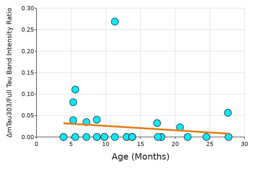
Figure 3. Age versus Δtau303 to full-length tau ratio band intensity in male and female brain samples from Tg2576 mice (n = 30; p = 0 50) Samples with intensities that were not significantly different from the background were set to zero for this analysis (Figure by authors).
Correlation of levels of Aβ*56 and Δtau303
There was no significant relationship between Aβ*56 band intensity and the ratio of Δtau303 to full-length tau (p = 0 49; Linear Regression; Figure 4).
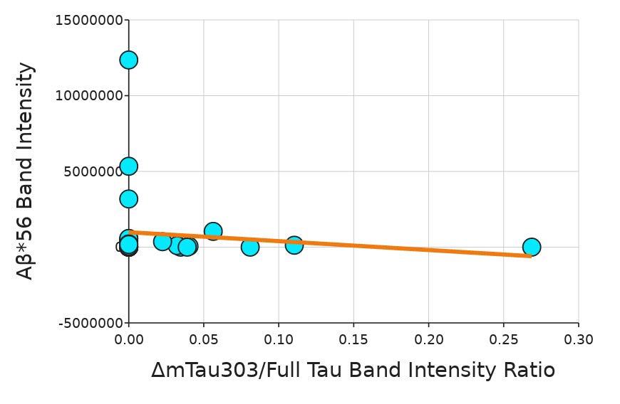
Figure 4. Aβ*56 band intensity versus Δtau303 to full-length tau ratio band intensity in male and female brain samples from Tg2576 mice (n = 30; p = 0.49). Samples with intensities that were not significantly different from the background were set to zero for this analysis (Figure by authors)
Discussion
We hypothesized that levels of Δtau303 are correlated with levels of Aβ*56 and both are elevated in an age-dependent manner in Tg2576 mice Aβ*56 expression levels increased in the brains of Tg2576 mice in an age-dependent manner, as previously reported (Liu et al., 2023). Interestingly, Δtau303 expression was only seen in Tg2576 mice, while all wild-type mice had no Δtau303 expression. However, there was no significant relationship between age and t he Δtau303/full tau ratio. Additionally, there was no significant relationship between levels of Aβ*56 and Δtau303/full tau ratio Fifteen (50%) of the samples were positive for Aβ*56 without having any detectable Δtau303 and only four samples were positive for Δtau303 without any detectable Aβ*56. Furthermore, there was no correlation between Aβ*56 and Δtau303 across all samples. Therefore, these results do not indicate a causal relationship between Aβ*56 and Δtau 303 or its human equivalent, Δtau314. The findings suggest that Aβ*56 and caspase-2-mediated tau cleavage may affect cognitive function through distinct molecular mechanisms.
Matthew Manacek and Samantha Dvorak
The mice used were collected at a range of ages with only a few samples at each age Moreover, the number of samples from each age group was inconsistent, with there being fewer mice aged 20 7 months to 27 7 months Additionally, the male-to-female ratio was inconsistent across age ranges. These discrepancies likely impacted the power of statistical analysis This investigation will need to be expanded to include a larger number of samples to verify and increase confidence in the conclusions
Further work in investigating the relationship between Aβ and tau should include comparing other versions of tau to Aβ*56 The presence of Δtau303 in the Tg2576 mice but not the wild-type mice suggests that it does play a part in Alzheimer’s pathology Future work could focus on investigating the role of this tau species. Because there are so many potential species involved in Alzheimer’s, ruling out ones that are not interacting is an important step toward understanding this complicated disease.
We would like to thank Dr Kati Kragtorp for her help in navigating science research and creating this research paper. We would also like to thank Dr Karen Ashe for the opportunity to work in her lab and the support she provided throughout our work. We would like to thank Lisa Kemper for the time she committed to teaching us these laboratory techniques and for her guidance throughout our time in the lab. Finally, we would like to thank Dr Peng Liu for his help in perfecting laboratory skills and analyzing data in addition to reviewing our manuscript.
Alzheimer’s Disease Facts and Figures (n d ) Alzheimer’s Disease and Dementia Retrieved June 17, 2023, from https://www alz org/alzheimers-dementia/facts-figures Amar, F , Sherman, M A , Rush, T , Larson, M , Boyle, G , Chang, L , Götz, J , Buisson, A , & Lesné, S E (2017) Amyloid-β oligomer Aβ*56 induces specific alterations of tau phosphorylation and neuronal signaling Science Signaling, 10(478), eaal2021 https://doi org/10 1126/scisignal aal2021
Asai, M , Hattori, C , Szabó, B , Sasagawa, N , Maruyama, K , Tanuma, S., & Ishiura, S. (2003). Putative function of ADAM9, ADAM10, and ADAM17 as APP-secretase Biochemical and Biophysical Research Communications, 301(1), 231–235 https://doi org/10 1016/S0006-291X(02)02999-6
Ashe, K H (2020) The biogenesis and biology of amyloid β oligomers in the brain Alzheimer’s & Dementia, 16(11), 1561–1567 https://doi org/10 1002/alz 12084
Avila, J., Lucas, J. J., Perez, M., & Hernandez, F. (2004). Role of tau protein in both physiological and pathological conditions Physiological Reviews, 84(2), 361–384 https://doi org/10 1152/physrev 00024 2003
Bernabeu-Zornoza, A , Coronel, R , Palmer, C , López-Alonso, V , & Liste, I (2021) Oligomeric and Fibrillar Species of Aβ42 Diversely Affect Human Neural Stem Cells International Journal of Molecular Sciences, 22(17), 9537. https://doi org/10 3390/ijms22179537
Breijyeh, Z , & Karaman, R (2020) Comprehensive Review on Alzheimer’s Disease: Causes and Treatment Molecules, 25(24), 5789 https://doi org/10 3390/molecules25245789
Briner, A , Götz, J , & Polanco, J C (2020) Fyn Kinase Controls Tau Aggregation In Vivo Cell Reports, 32(7), 108045 https://doi.org/10.1016/j.celrep.2020.108045
Hsiao, K , Chapman, P , Nilsen, S , Eckman, C , Harigaya, Y , Younkin, S , Yang, F , & Cole, G (1996) Correlative memory deficits, Abeta elevation, and amyloid plaques in transgenic mice Science (New York, N Y ), 274(5284), 99–102 https://doi org/10 1126/science 274 5284 99
Iijima, K., Gatt, A., & Iijima-Ando, K. (2010). Tau Ser262 phosphorylation is critical for Aβ42-induced tau toxicity in a transgenic Drosophila model of Alzheimer’s disease Human Molecular Genetics, 19(15), 2947–2957 https://doi org/10 1093/hmg/ddq200
Lilek, J , Ajroud, K , Feldman, A Z , Krishnamachari, S , Ghourchian, S , Gefen, T , Spencer, C L , Kawles, A , Mao, Q , Tranovich, J F , Jack, C R , Mesulam, M -M , Reichard, R R , Zhang, H., Murray, M. E., Knopman, D., Dickson, D. W., Petersen, R C , Smith, B , Flanagan, M E (2023) Accumulation of pTau231 at the Postsynaptic Density in Early Alzheimer’s Disease Journal of Alzheimer’s Disease, 92(1), 241–260 https://doi org/10 3233/JAD-220848
Liu, P , Smith, B R , Huang, E S , Mahesh, A , Vonsattel, J P G , Petersen, A J , Gomez-Pastor, R , & Ashe, K H (2019) A soluble truncated tau species related to cognitive dysfunction and caspase-2 is elevated in the brain of Huntington’s disease patients Acta Neuropathologica Communications, 7(1), 111 https://doi org/10 1186/s40478-019-0764-9
Liu, P , Smith, B R , Montonye, M L , Kemper, L J , Leinonen-Wright, K , Nelson, K M , Higgins, L , Guerrero, C R , Markowski, T W , Zhao, X , Petersen, A J , Knopman, D S , Petersen, R C , & Ashe, K H (2020) A soluble truncated tau species related to cognitive dysfunction is elevated in the brain of cognitively impaired human individuals Scientific Reports, 10(1), 3869 https://doi org/10 1038/s41598-020-60777-x
Mairet-Coello, G , Courchet, J , Pieraut, S , Courchet, V , Maximov, A , & Polleux, F (2013) The CAMKK2-AMPK kinase pathway mediates the synaptotoxic effects of Aβ oligomers through
Tau phosphorylation Neuron, 78(1), 94–108 https://doi.org/10.1016/j.neuron.2013.02.003
Ossenkoppele, R , Smith, R , Ohlsson, T , Strandberg, O , Mattsson, N , Insel, P S , Palmqvist, S , & Hansson, O (2019) Associations between tau, Aβ, and cortical thickness with cognition in Alzheimer disease Neurology, 92(6), e601–e612 https://doi org/10 1212/WNL 0000000000006875
Rissman, R A , Poon, W W , Blurton-Jones, M , Oddo, S , Torp, R., Vitek, M. P., LaFerla, F. M., Rohn, T. T., & Cotman, C. W. (2004) Caspase-cleavage of tau is an early event in Alzheimer disease tangle pathology Journal of Clinical Investigation, 114(1), 121–130 https://doi org/10 1172/JCI200420640
Vassar, R , Bennett, B D , Babu-Khan, S , Kahn, S , Mendiaz, E A , Denis, P , Teplow, D B , Ross, S , Amarante, P , Loeloff, R , Luo, Y , Fisher, S , Fuller, J , Edenson, S , Lile, J , Jarosinski, M A., Biere, A. L., Curran, E., Burgess, T., … Citron, M. (1999). β-Secretase Cleavage of Alzheimer’s Amyloid Precursor Protein by the Transmembrane Aspartic Protease BACE Science, 286(5440), 735–741 https://doi org/10 1126/science 286 5440 735
Westerman, M A , Cooper-Blacketer, D , Mariash, A , Kotilinek, L , Kawarabayashi, T , Younkin, L H , Carlson, G A , Younkin, S G , & Ashe, K H (2002) The Relationship between Aβ and Memory in the Tg2576 Mouse Model of Alzheimer’s Disease The Journal of Neuroscience, 22(5), 1858–1867 https://doi org/10 1523/JNEUROSCI 22-05-01858 2002
Wolfe, M S (2008) Inhibition and Modulation of γ-Secretase for Alzheimer’s Disease Neurotherapeutics, 5(3), 391–398 https://doi org/10 1016/j nurt 2008 05 010
Zempel, H , Thies, E , Mandelkow, E , & Mandelkow, E -M (2010). Abeta oligomers cause localized Ca(2+) elevation, missorting of endogenous Tau into dendrites, Tau phosphorylation, and destruction of microtubules and spines The Journal of Neuroscience: The Official Journal of the Society for Neuroscience, 30(36), 11938–11950 https://doi org/10 1523/JNEUROSCI 2357-10 2010
Zhang, H , Jiang, X , Ma, L , Wei, W , Li, Z , Chang, S , Wen, J , Sun, J , & Li, H (2022) Role of Aβ in Alzheimer’s-related synaptic dysfunction Frontiers in Cell and Developmental Biology, 10, 964075 https://doi org/10 3389/fcell 2022 964075
Zhao, X , Kotilinek, L A , Smith, B , Hlynialuk, C , Zahs, K , Ramsden, M , Cleary, J , & Ashe, K H (2016) Caspase-2 cleavage of tau reversibly impairs memory Nature Medicine, 22(11), 1268–1276 https://doi org/10 1038/nm 4199
Corinne Moran
Is transient expression of the DUX4 gene sufficient to cause muscular dystrophy?
Corinne Moran
Introduction
Facioscapulohumeral muscular dystrophy (FSHD) is a genetic, progressive myopathy and the second most common muscular dystrophy. Progression of the disease primarily begins with the weakening and atrophy of facial, shoulder, and upper arm skeletal muscles. However, advancement may affect other parts of the body, causing respiratory and cardiac issues (Schätzl et al., 2021). The disease typically begins presenting in the second decade of a patient's life, though some cases see symptom onset in infancy. Those afflicted with the disease from an early age typically develop a more severe form compared to other patients FSHD has a highly complex pathology, combining mechanics of both genetics and epigenetics. Thus, severity differs from patient to patient, though it does not seem to affect life expectancy (Himeda & Jones, 2019).
There are two main forms of FSHD, caused by two different genetic mechanisms: FSHD1 and FSHD2. FSHD1 is the more common of the two, affecting 95% of all FSHD patients, and is caused by a contraction of CpG repeats on the D4Z4 array. This array typically consists of 11-100 repeat units but is contracted to 1-10 repeat units in FSHD1 patients FSHD2 affects about 5% of all patients and is most commonly caused by a mutation in the gene SMCHD1, leading to another contraction of repeats (Himeda & Jones, 2019; Le Gall et al., 2020). Despite these differences, both mechanisms lead to the derepression of the double homeobox protein 4 gene (DUX4). Aberrant expression of DUX4 in muscle cells is widely believed to be the primary cause of the FSHD phenotype (Bosnakovski et al., 2008).

Normally only expressed during the cleavage stage in embryonic development, as well as the testis and thymus, DUX4 is epigenetically repressed by the D4Z4 repeat (Yoshihara et al., 2022) When that repeat is contracted, the gene is no longer repressed and initiates this same program in muscle cells (myoblasts). The DUX4 gene codes for both a short form DUX4 (DUX4-s), which does not activate DUX4 target genes, and a full-length DUX4 (DUX4-fl), which acts as a transcription factor for numerous target genes (Bosnakovski et al , 2020) DUX4-s lacks the C-terminus present on DUX4-fl, which is the transcriptional activator domain of the gene (Choi et al , 2016) The target genes that DUX4-fl activates are associated with cell death, oxidative stress, muscle generation and growth (myogenesis), epigenetic regulation, and multiple other skeletal muscle pathways (Bosnakovski et al , 2008)
Interestingly, although DUX4 is considered the primary cause of FSHD, it's often undetectable, or detectable only at very low levels, in FSHD patient muscles (Banerji & Zammit, 2021) Its expression is so elusive that researchers routinely use the activation of DUX4 target genes to detect the expression of DUX4 itself (Lim et al., 2020). For this reason, it is hypothesized that instead of being expressed continuously in muscle cells, which has severely cytotoxic effects, DUX4 is expressed transiently and at very low levels, with downstream target genes leading to a long-term decline in muscle cell viability. This hypothesis, however, has yet to be fully demonstrated in an experimental model of the disease The inability to observe DUX4 expression in FSHD patients necessitates effective disease modeling to understand the complex relationships between various genes and transcription factors in FSHD pathology.
Most animal models of FSHD are in mice, though xenograft, Drosophila, and zebrafish models have been developed as well (Le Gall et al., 2020). However, animal models have proved more difficult to develop than cell models because of the cytotoxic nature of DUX4 (Le Gall et al., 2020). Additionally, none of these models faithfully recapitulate the DUX4 promoter, DUX4 mRNA, DUX4 protein, or fully represent disease progression. As DUX4 is a primate-specific gene, expression in n on-primate organisms causes cytotoxicity and death In recent years, researchers have mitigated this issue by creating inducible animal models, to control the level and duration of DUX4 expression such that the animal survives the testing period (Le Gall et al , 2020) However, these inducible animal models have proved unreliable. The mouse model, iDUX4, exhibited a leaky expression of DUX4, meaning the gene activated not only in muscle cells, but, uncontrollably, in other parts of the mouse as well (Dandapat et al , 2014) Consequently, this group turned to the iDUX4pA-HSA mouse model, which eliminated the leaky expression, but raised another issue, as the majority of muscle cells were not positive for DUX4 expression (Bosnakovski et al., 2017).
Though animal models are useful, cell models have the advantage of helping researchers study how DUX4 works with greater precision, on the cellular level. This creates a better platform to work toward recapitulating DUX4 expression levels in different human types of myoblasts and fibroblasts. Previous experiments used the cell line C2C12, a murine cell line, in order to induce DUX4 expression and follow the disease (Bosnakovski et al., 2008). The issue with this approach is that DUX4 is not typically induced in mice, so some interactions of DUX4 in human cells are not present in murine cells, and thus such models are not a perfect recapitulation of the human disease (Sharma et al., 2013). To better represent disease pathology, the Kyba lab developed an immortalized human myoblast iDUX4 cell line in which DUX4 expression is induced by doxycycline, an antibiotic that binds to the gene promoter (Bosnakovski et al , 2018)
In studies which have used the inducible cell line approach to research DUX4’s expression platform, signaling pathways, and transcriptional activity, a common setback is that cells fail to survive more than 48 hrs after DUX4 is expressed, due to the gene’s cytotoxic effects (Bosnakovski et al., 2019). This hinders such models’ ability to investigate transient DUX4 expression’s long term effects on target gene regulation, a key component to understanding FSHD pathology
I developed and optimized a transient cell assay of DUX4 in vitro, using the human myoblast cell line LHCN #3 iDUX4, to investigate whether low level, transient expression of DUX4 was sufficient to sustain increased expression of target genes associated with the FSHD genotype, while avoiding immediate cell death, and how expression of the DUX4 pathway affected long term cell viability. Low level, transient DUX4 expression significantly increased the expression of a number of DUX4 target genes for a prolonged period, causing proportional cytotoxicity and injury to cells This research represents an important step toward clarifying the mechanism behind FSHD and eventually developing effective FSHD therapies
Materials and Methods
Cell Culture
Immortalized human myoblasts from the LHCN #3 iDUX4 cell line were cultured in myogenic proliferation media [F10 (HyClone) supplemented with 20% fetal bovine serum (FBS; Peak Serum, Ps-FB3, lot 293Q16), 1× 2-mercaptoethanol (Gibco), 10 9 M dexamethasone (Sigma Aldrich), basic fibroblast growth factor (10 ng/ml; PeproTech), GlutaMAX (Gibco), and penicillin/streptomycin (Gibco)], at 37°C in a 5% CO2 atmosphere (Bosnakovski et al, 2016) The immortalized human myoblast cell line, LHCN #3 iDUX4, was developed from the immortalized LHCN-M2 cell line obtained from V Mouly (Toral-Ojeda et al , 2018), by transduction with a single copy of DUX4 downstream of a second-generation tet response element (Choi et al , 2016)
Corinne Moran
Cells were plated in T-75 flasks, with media changed every three days until confluence, then plated in 12, 24, 48, or 96 well plates for further experimentation.
When experimentation plate wells reached confluence, DUX4 expression was induced in the LHCN iDUX4 cells by adding a 12.5 ng/ml, 50 ng/ml, or 200 ng/ml dilution of doxycycline (Dox.; Sigma Aldrich) in myogenic media, for a pulse induction time of 30 or 60 minutes. A negative control was established with no doxycycline pulse and incubated until data collection, while a positive control was set up with continuous doxycycline exposure and incubated until data collection. After the pulse induction time had passed, the doxycycline dilution was removed from the experimental group. All cells were washed twice with Dulbecco's Modified Eagle Medium (DMEM; Cytiva), and replaced with myogenic media, except for the positive control group, which experienced continued exposure to doxycycline
RNA extraction
RNA was extracted directly from the plate at 1, 2, 4, 8, 12, 24., 36, 48, 60, 72, and 96 hrs. post pulse induction Media was aspirated from plate wells, and cells were treated with equal amounts of lysis buffer (Zymo Research) and 70% ethanol The lysate was then transferred to filter tubes and RNA was extracted using the Quick RNA mini-prep kit (Zymo Research), according to the manufacturer's instructions
cDNA synthesis
cDNA was synthesized from the extracted RNA using the Verso kit (Thermo Fisher Scientific) with 4 µl of 5x buffer, 2 µl of dNTP, 1 µl of Oligo, 0.5 µl of RT enhancer, and 0.5 µl of RT enzyme per same, and 12 µl of water and RNA The resulting solution was placed in a thermocycler (Bio-Rad) at a cycle of 42°C for 1 hr., and 95°C for 2 minutes, then held at 4°C
cDNA was prepared for qPCR using the Terra qPCR direct TB Green Premix (Takara), and gene expression was measured with commercially available probes: ZSCAN4, Hs00537549 m1; MBD3L2, HS00544743 m1; LEUTX, Hs01028718 m1; TRIM43, Hs00299174 m1; SLC34A2, Hs00197519 m1; DUX4, Hs07287098 g1; B2M, Hs99999907 m1 (Applied Biosystems) Gene expression levels were normalized to B2M and analyzed with 7500 System Software (Applied Biosystems)
Statistical analysis was performed by conducting t-tests between any compared data groups.
Media was aspirated from cell culture plates, then enough 4% paraformaldehyde (PFA) to cover the bottom of each well was added for 10 minutes before aspiration Enough 1x phosphate buffered saline (PBS) to cover the bottom of each well was then added for 30 minutes, then aspirated, then enough 0 3% TritonX to cover the bottom of each well was added for 1 hr. before being aspirated. Finally, commercially available primary antibodies [Rabbit Polyclonal Anti-SLC34A2 Antibody (RayBiotech); Mouse anti-Human Dux4, MABD116 (Millipore Sigma)] were diluted in 3% bovine serum albumin (BSA), each to a 1:500 concentration, added to each well, and the plate was stored at 4°C overnight The following day, plates were washed with 1x PBS twice, for 5 minutes each time, before commercially available fluorochrome-conjugated secondary antibodies [Goat anti-Rabbit IgG, AB 143157; Donkey anti-Mouse IgG, AB 2536180 (Invitrogen)] were diluted in 3% BSA to a 1:500 concentration and added to each well for 1 hr.. Pla tes were then washed with PBS three times, for 5 minutes each time, before 4′,6-diamidino -2-phenylindole (DAPI; Sigma-Aldrich) was added to each well for 10 minutes. Plates were washed with PBS for 5 minutes before being stored in PBS at 4°C. Plate images were taken on a Zeiss microscope and analyzed with ZEN Microscopy Software (ZEISS) ImageJ was then used to quantify the percentage of activated
cells, with statistical analysis performed by conducting t-tests between any compared data groups
Cultured cells used for experimentation were trypsinized and suspended in a sterile propidium iodide solution. Cells were then stained with the commercially available primary and antibody antibodies [Rabbit Polyclonal Anti-SLC34A2 Antibody (RayBiotech); Goat anti-Rabbit IgG, AB 143157 (Invitrogen)] diluted in 3% BSA each to a 1:500 concentration, and washed twice with PBS before being resuspended in PBS for analysis Stained samples were run on a BD FACSAria instrument, and data was analyzed using FlowJo (BD Biosciences).
Activation of DUX4 expression
In a 24-well plate, there were six wells per treatment group of LHCN iDUX4 cells pulsed with varying doxycycline concentrations for 30 minutes Six wells were pulsed with 12 5 ng/ml doxycycline, six were pulsed with 50 ng/ml doxycycline, six were pulsed with 200 ng/ml doxycycline, and another six wells were left untreated as a negative control. Immunofluorescence images were taken at 1 and 4 hrs to quantify DUX4 protein presence The percentage of cells expressing DUX4 increased with pulse concentration and time post-pulse (Table 1)
Table 1. Percentage of cells expressing DUX4, 1 and 4 hrs. after 30 minute doxycycline pulses of varying concentrations
Doxycycline pulse concentration
Percentage of cells expressing DUX4, 1 hr post-pulse
Percentage of cells expressing DUX4, 4 hrs post-pulse
Levels of DUX4 mRNA were assessed in cells 1, 2, 4, 8, 12, 24 , 36, 48, 60, 72, and 96 hrs after a 30 minute pulse of 50 ng/ml doxycycline Levels of DUX4 mRNA were significantly different in treated cells as compared to untreated cells at the 12 hr (p < 0 05), 36 hr (p < 0.05), 48 hr. (p < 0.01), and 60 hr. (p < 0.005) time points In the treated cells, DUX4 expression levels significantly decreased from 24 to 36 hrs. (p < 0.05), and from 60 hrs. to 72 hrs. (p < 0 05) While the differences in levels of DUX4 mRNA were not significant between hr 1 and hr. 2 or between treated and untreated cells at hr 1, treated cells at hr 1 had the highest DUX4 mRNA levels of any sample (Figure 1) The lack of statistical difference in DUX4 expression between treated and untreated cells at hr 1 is likely due to skew from an outlier control sample in which m RNA levels were tenfold that of all other control samples Interestingly, the statistically insignificant increase in DUX4 mRNA at hr. 1 succeeded in activating the DUX4 pathway, emphasizing the ability for minimally elevated levels of transient DUX4 expression to effectively induce markers of the FSHD phenotype
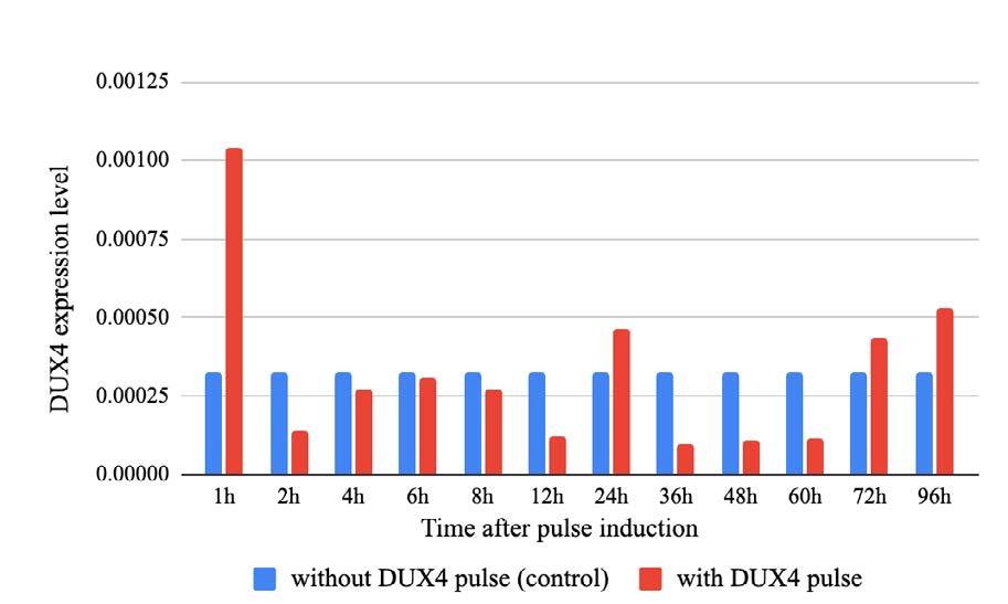
Figure 1. Levels of DUX4 mRNA in cells with (red) and without (blue) a 30 minute pulse induction of 50 ng/ml doxycycline. Cells collected at 1, 2., 4, 8, 12, 24, 36, 48, 60, 72, and 96 hrs post pulse induction (Figure by author)
The percentage of cells positive for DUX4 protein was quantified through immunofluorescence imaging at 1, 2, 4, 8, 12, 24 , 36, 48, 60, 72, and 96 hrs after a 30-minute pulse of 50 ng/ml doxycycline. DUX4 protein presence peaked at 4 hrs post pulse, with 4 93%
Corinne Moran
of cells positive for DUX4, before quickly sinking to 0 37% at 8 hrs , and disappearing completely at 72 hrs (Figure 2; Figure 3)
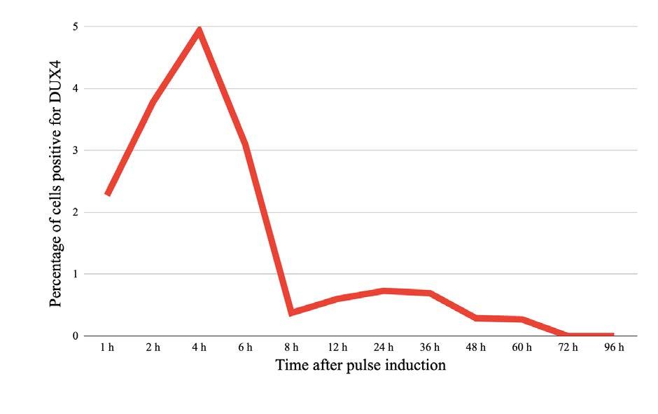
Figure 2. Percentage of cells positive for the DUX4 protein following a 30 minute pulse induction of 50 ng/ml doxycycline Cells imaged at 1, 2 , 4, 8, 12, 24, 36, 48, 60, 72, and 96 hrs post pulse induction (Figure by author).

Figure 3. Example immunofluorescence images of cells without (A) and with (B) a 30-minute pulse induction of 50 ng/ml doxycycline, stained for the DUX4 protein (red) and nuclei counterstained with DAPI (blue), 2 hrs post pulse induction (Figure by author)
Cells were analyzed through FACS to determine the percentage of cells positive for DUX4 target SLC34A2, and the percentage of dead cells, 24 hrs after doxycycline pulses of varying concentrations and durations (Table 2). The percentage of cells positive for SLC34A2 rose with the concentration and duration of the doxycycline pulse, and the percentage of dead cells increased with doxycycline pulse concentration (Table 2) Interestingly, unlike SLC34A2 activation, cell death did not increase between cells treated with 50 ng/ml dox. for 30 minutes and 60 minutes (Table 2)
While the large majority of cells survived for 24 hrs post pulse induction under all induction
conditions, almost all cells failed to reattach when replated after cell sorting, while uninduced control cells were able to reattach as normal (Figure 4).
Table 2. Percentage of cells positive for DUX4 target SLC34A2 and percentage of dead cells, 24 hrs. after doxycycline pulses of varying concentrations and durations
Doxycycline pulse concentration (duration)
Percentage of cells positive for SLC34A2
of dead cells

Figure 4. Example immunofluorescence images of cells without (A) and with (B) a 30-minute pulse induction of 50 ng/ml doxycycline, nuclei stained with DAPI (blue), 48 hrs post pulse induction and 24 hrs post trypsinization and replating (Figure by author).
Cells pulsed with 50 ng/ml doxycycline for 30 minutes were immunostained for DUX4 and target gene SLC34A2 product proteins before immunofluorescence images were taken of the cells at 1 hr , 2 hrs , 4 hrs , 8 hrs , 12 hrs , 24 hrs., 36 hrs., 48 hrs., 60 hrs., 72 hrs., and 96 hrs. post pulse induction. These images were then quantified to determine the percentage of cells positive for DUX4 and SLC34A2 proteins. DUX4 protein presence peaked first at 4 hrs. post pulse, with 4 93% of cells positive for DUX4, before quickly sinking to 0.37% at 8 hrs., and disappearing completely at 72 hrs. SLC34A2 protein presence peaked later, at 8 hrs post pulse, with 4.12% of cells positive for SLC34A2, before its presence gradually
declined to 0.61% at 96 hrs. post pulse (Figure 5; Figure 6)
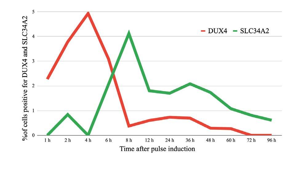
and SLC34A2 proteins following a 30-minute pulse induction of 50 ng/ml doxycycline Cells imaged at 1, 2 , 4, 8, 12, 24, 36, 48, 60, 72, and 96 hrs post pulse induction (Figure by author)
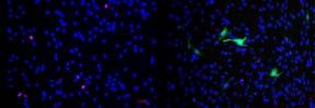
Figure 6. Example immunofluorescence images of cells 4 hrs. (A) and 8 hrs. (B) after a 30-minute pulse induction of 50 ng/ml doxycycline, stained for the DUX4 protein (red), SLC34A2 protein (green), and nuclei counterstained with DAPI (blue; Figure by author)
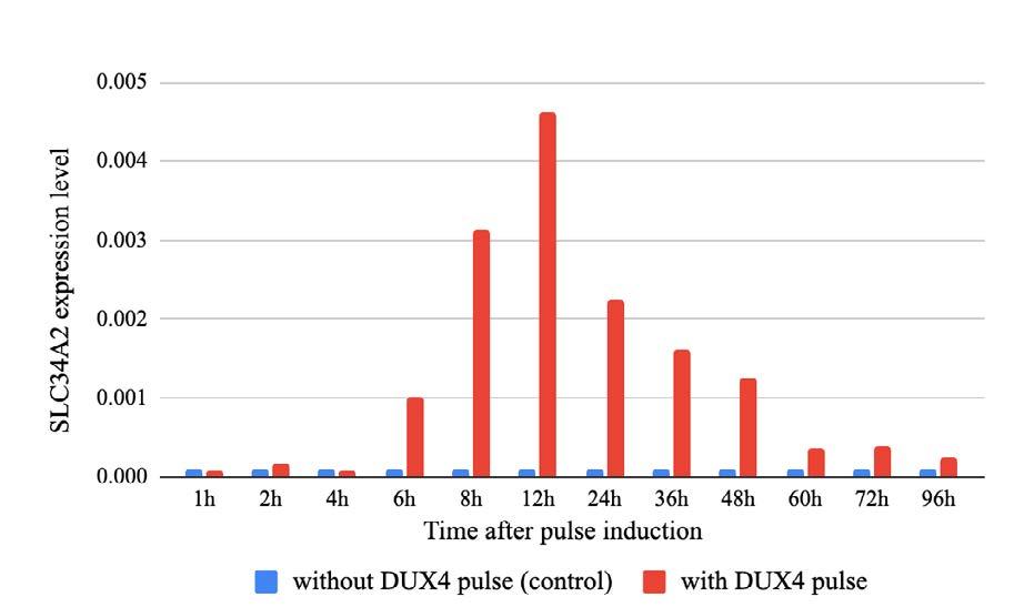
Figure 7. Levels of SLC34A2 mRNA in cells with (red) and without (blue) a 30 minute pulse induction of 50 ng/ml doxycycline Samples collected at 1, 2 , 4, 8, 12, 24, 36, 48, 60, 72, and 96 hrs. post pulse induction (Figure by author).
Levels of SLC34A2 mRNA were also assessed in cells 1, 2, 4, 8, 12, 24 , 36, 48, 60, 72, and 96 hrs. after a 30 minute pulse of 50 ng/ml
doxycycline. Levels of SLC34A2 mRNA were significantly different in treated cells as compared to untreated cells at the 6 hr (p < 0.05), 8 hr. (p < 0.05), 12 hr. (p < 0.05), 24 hr. (p < 0 005), 36 hr (p < 0 005), 60 hr (p < 0 05), and 72 hr (p < 0 05) time points (Figure 7)
The mRNA of all downstream DUX4 target genes analyzed in this study (SLC34A2, LEUTX, ZScan4c, TRIM43, and MBD3L2), following a 30-minute pulse induction of 50 ng/ml doxycycline, were noticeably height ened as compared to control levels, while DUX4 mRNA itself was not With target genes’ mRNA levels in treated cells expressed as a percent change of levels in untreated cells so as to compare the activation of downstream targets, similar expression patterns are observable along a varied timeline. All target genes’ mRNA expression levels increased and then regressed back towards their control levels, with the only difference being the length of time after DUX4 pulse induction that their expression peaks (Figure 8) The variation in delay of DUX4 target gene activation indicates potential for interaction between these downstream targets, providing a basis for further study of the potential relationships between downstream genes in the DUX4 pathway
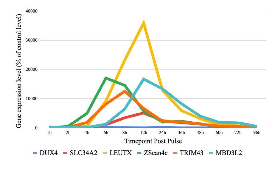
Figure 8. Levels of DUX4 (blue), SLC34A2 (red), LEUTX (yellow), ZScan4c (green), TRIM43 (orange), and MBD3L2 (light blue) mRNA in cells following a 30 minute pulse induction of 50 ng/ml doxycycline Samples collected at 1, 2., 4, 8, 12, 24, 36, 48, 60, 72, and 96 hrs. post pulse induction (Figure by author).
Corinne Moran
As hypothesized, a doxycycline concentration of 50 ng/ml and treatment duration of 30 minutes produced optimal induction of transient DUX4 in the human myoblast cell line LHCN #3 iDUX4. This protocol generated a minimal burst of activation, increasing DUX4 gene expression in only a small percentage of cells, primarily in the first hour, and creating a short-term expression of the DUX4 product protein Additionally, this low-level, transient expression of DUX4 was sufficient to sustain increased expression of target genes associated with the FSHD genotype as expected Target genes SLC34A2, LEUTX, ZScan4c, TRIM43, and MBD3L2 all demonstrated significantly heightened expression for multiple days following a 30-minute pulse of DUX4 induction. With expression of the DUX4 pathway, however, the model was not fully able to avoid immediate cell death. While cells survived significantly longer than 48 hrs , surpassing previous models, DUX4 expression still led to cytotoxicity, and interestingly, significant injury to cell function.
Although the extended period of cell viability is promising, the cytotoxicity observed is still a barrier to accurately understanding the relationships between DUX4 and its target genes The direct correlation between increased doxycycline concentration for induction and increased cell death at 24 hrs post pulse indicates a relationship between DUX4 pathway expression and immediate cytotoxicity. Additionally, the inability of induced cells to reattach to a plate after trypsinization indicates large-scale cell damage, potentially limiting cell proliferation If cells expressing the DUX4 pathway constitute a larger proportion of observed cell death, and smaller proportion of proliferating cells, the ratio of uninduced cells to DUX4-induced cells increases as the experiment progresses, skewing results and interfering with our ability to accurately detail the complex transcriptional interactions of DUX4 and its target genes. Across all target genes examined in this study, mRNA was still significantly heightened 72 hrs post pulse induction, but was in decline. While this decrease could be natural
in the absence of upstream signaling, it is likely attributable in at least part to the cytotoxic effects of DUX4 expression The lack of clarity as to exactly how much cell death alters the results of other measurements leaves a gap in our understanding of the reality of FSHD pathology. Unfortunately, while a hindrance to sustainable disease models, DUX4’s cytotoxic effects are a key component of FSHD itself, and may be unavoidable, even at increasingly low levels of DUX4 expression It is also worth noting that other limitations of this cell model include its inability to account for DUX4 interactions with other cell types and interference in non-myogenic processes
This study’s finding that low-level transient DUX4 expression significantly increases the expression of a number of DUX4 target genes for a prolonged period, causing proportional cytotoxicity and injury to cells, provides novel evidence for the hypothesis that FSHD pathology is dependent of transient DUX4 expression causing cell death and decreased proliferation This research represents an important step toward clarifying the mechanism behind FSHD and eventually developing effective FSHD therapies
In the future, I look to develop a more detailed understanding of the relationship between specific DUX4 target gene expression, cell injury, loss of proliferation ability, and cell death In hand with studies such as this to understand the timeline of the DUX4 pathway, greater knowledge of target gene’s effects would allow for more accurate construction of FSHD pathology Next steps include using flow cytometry, rt-qPCR, or immunohistochemistry to determine the percentage of effectively induced LHCN iDUX4 cells which sustain injury or die as time progresses, as compared to uninduced cells Additionally, isolating specific target genes and candidate upstream factors in similar cell model systems may allow for a more focused analysis of any given genetic relationship While continued research of FSHD pathology using in vitro cell models is crucial for future in vivo
studies, it may be beneficial to utilize models co-culturing different cell types, cell transplants, and locally inducible animal models for a more sustainable system.
First and foremost, I thank Dr Kati Kragtorp for her guidance in research and academic writing, as well as my peers, whose invaluable feedback has allowed me to effectively communicate the following findings I also wish to thank my mentor and University of Minnesota Department of Pediatrics Assistant Professor Dr Darko Bosnakovski, who opened the doors to his lab and allowed me the opportunity to conduct this research My work would not have been possible without his generous support, the contributions of the Bosnakovski lab as a whole, and the resources of the Cancer and Cardiovascular Research Building
Banerji, C R S , & Zammit, P S (2021) Pathomechanisms and biomarkers in facioscapulohumeral muscular dystrophy: Roles of DUX4 and PAX7 EMBO Molecular Medicine, 13(8), e13695 https://doi.org/10.15252/emmm.202013695
Bosnakovski, D , Chan, S S K , Recht, O O , Hartweck, L M , Gustafson, C J , Athman, L L , Lowe, D A , & Kyba, M (2017) Muscle pathology from stochastic low level DUX4 expression in an FSHD mouse model Nature Communications, 8(1), 550 https://doi org/10 1038/s41467-017-00730-1
Bosnakovski, D., da Silva, M. T., Sunny, S. T., Ener, E. T., Toso, E. A , Yuan, C , Cui, Z , Walters, M A , Jadhav, A , & Kyba, M (2019) A novel P300 inhibitor reverses DUX4-mediated global histone H3 hyperacetylation, target gene expression, and cell death Science Advances, 5(9), eaaw7781 https://doi org/10 1126/sciadv aaw7781
Bosnakovski, D , Gearhart, M D , Toso, E A , Ener, E T , Choi, S H , & Kyba, M (2018) Low level DUX4 expression disrupts myogenesis through deregulation of myogenic gene expression. Scientific Reports, 8, 16957 https://doi org/10 1038/s41598-018-35150-8
Bosnakovski, D , Shams, A S , Yuan, C , Silva, M T da, Ener, E T , Baumann, C W , Lindsay, A J , Verma, M , Asakura, A , Lowe, D A , & Kyba, M (2020) Transcriptional and cytopathological hallmarks of FSHD in chronic DUX4-expressing mice The Journal of Clinical Investigation, 130(5), 2465–2477. https://doi org/10 1172/JCI133303
Bosnakovski, D , Xu, Z , Ji Gang, E , Galindo, C L , Liu, M , Simsek, T , Garner, H R , Agha-Mohammadi, S , Tassin, A , Coppée, F , Belayew, A , Perlingeiro, R R , & Kyba, M (2008) An isogenetic myoblast expression screen identifies DUX4-mediated FSHD-associated molecular pathologies The
EMBO Journal, 27(20), 2766–2779 https://doi.org/10.1038/emboj.2008.201
Choi, S H , Gearhart, M D , Cui, Z , Bosnakovski, D , Kim, M , Schennum, N , & Kyba, M (2016) DUX4 recruits p300/CBP through its C-terminus and induces global H3K27 acetylation changes Nucleic Acids Research, 44(11), 5161–5173
https://doi org/10 1093/nar/gkw141
Dandapat, A , Bosnakovski, D , Hartweck, L M , Arpke, R W , Baltgalvis, K. A., Vang, D., Baik, J., Darabi, R., Perlingeiro, R. C. R , Hamra, F K , Gupta, K , Lowe, D A , & Kyba, M (2014) Dominant Lethal Pathologies in Male Mice Engineered to Contain an X-Linked DUX4 Transgene Cell Reports, 8(5), 1484–1496 https://doi org/10 1016/j celrep 2014 07 056
Himeda, C L , & Jones, P L (2019) The Genetics and Epigenetics of Facioscapulohumeral Muscular Dystrophy Annual Review of Genomics and Human Genetics, 20(1), 265–291. https://doi org/10 1146/annurev-genom-083118-014933
Le Gall, L , Sidlauskaite, E , Mariot, V , & Dumonceaux, J (2020) Therapeutic Strategies Targeting DUX4 in FSHD Journal of Clinical Medicine, 9(9), 2886 https://doi org/10 3390/jcm9092886
Lim, K R Q , Nguyen, Q , & Yokota, T (2020) DUX4 Signalling in the Pathogenesis of Facioscapulohumeral Muscular Dystrophy International Journal of Molecular Sciences, 21(3), 729. https://doi org/10 3390/ijms21030729
Schätzl, T , Kaiser, L , & Deigner, H -P (2021) Facioscapulohumeral muscular dystrophy: Genetics, gene activation and downstream signalling with regard to recent therapeutic approaches: an update Orphanet Journal of Rare Diseases, 16(1), 129 https://doi org/10 1186/s13023-021-01760-1
Sharma, V , Harafuji, N , Belayew, A , & Chen, Y -W (2013) DUX4 differentially regulates transcriptomes of human rhabdomyosarcoma and mouse C2C12 cells PloS One, 8(5), e64691 https://doi org/10 1371/journal pone 0064691
Toral-Ojeda, I , Aldanondo, G , Lasa-Elgarresta, J , Lasa-Fernandez, H , Vesga-Castro, C , Mouly, V , Munain, A L de, & Vallejo-Illarramendi, A (2018) A Novel Functional In Vitro Model that Recapitulates Human Muscle Disorders. In K. Sakuma (Ed ), Muscle Cell and Tissue Current Status of Research Field InTech https://doi org/10 5772/intechopen 75903
Yoshihara, M , Kirjanov, I , Nykänen, S , Sokka, J , Weltner, J , Lundin, K , Gawriyski, L , Jouhilahti, E -M , Varjosalo, M , Tervaniemi, M H , Otonkoski, T , Trokovic, R , Katayama, S , Vuoristo, S , & Kere, J (2022) Transient DUX4 expression in human embryonic stem cells induces blastomere-like expression program that is marked by SLC34A2 Stem Cell Reports, 17(7), 1743–1756 https://doi org/10 1016/j stemcr 2022 06 002
Charlotte Vasicek and Michael Setterberg
Charlotte Vasicek and Michael Setterberg
Introduction
Cancer is the second leading cause of death in the United States of America Affecting all age groups, the number of cancer diagnoses each year is projected to increase to 21 million by 2030 (Siegel et al , 2023) Improved detection and treatment is increasing the rate of survival in these growing case numbers, but existing treatments often have challenging side effects (Miller et al., 2022). In addition, obstacles like the COVID-19 pandemic can delay detection and treatment of cancer (Siegel et al , 2023) Thus, improving treatment and minimizing its side effects is a priority.
Malignant cells are constantly circulating in the body, and are identified by T cells through antigen presentation. Normally, T cells constantly surveil for diseased cells, and can recognize a specific antigen using their T cell receptors (TCR; Kumar et al., 2018). After antigen recognition, a cell-mediated immune response can eliminate the diseased cell The development of clinical cancer, called tumor escape, occurs when cancer cells develop traits that prevent the immune system from eliminating them. This involves changes such as the loss of cancer antigen expression and creation of an immunosuppressive tumor microenvironment (Hanahan & Weinberg, 2011)
Immunotherapies that stimulate an immune response to treat the disease have become an important subject of cancer treatment research One T cell-redirecting immunotherapy is chimeric antigen receptor (CAR)-T cells, which are patient-derived T cells that have been genetically modified to express a cancer antigen- targeting receptor (Kilic et al., 2020). However, the process of T cell isolation and modification has

many steps. The therapy must also be personalized to the individual patient, making it expensive and not easily accessible to all patients. Furthermore, CAR-T treatment has the potential to trigger cytokine release syndrome (Li et al , 2020) Another T cell immunotherapy is bispecific antibody therapy. Bispecific antibodies are engineered antibodies capable of binding to two antigens simultaneously, allowing them to bind to T cell surface antigens and connect the T cells to cancer cell antigens on the cancer cell surface While bispecific antibodies do not necessarily require patient T cell isolation, their size of about 50-60 kilodaltons (kDa) can lead to the treatment being filtered out of the blood after systemic administration and before reaching the site of the cancer (Van De Donk & Zweegman, 2023) They have also shown similar issues of cytokine release syndrome to CAR-T cell treatments (Van De Donk & Zweegman, 2023)
An alternative approach to immunotherapy currently being investigated is CSANs. CSANs are comprised of antibody fragments connected to the dimeric linking enzyme dihydrofolate reductase (DHFR2 or 1DD) that allow the antibody fragment-enzyme conjugates to form rings when triggered by a chemical oligomerizer. Previously, CSANs have been prepared using scFvs, which bind to surface TCRs, linked with scFvs that bind to a cancer antigen presented on the cancer cell surface. The scFvs targeting the TCR, as well as the scFvs targeting a cancer antigen, form into rings with the addition of chemical dimerizer bis-methotrexate (Li et al., 2010) Bis-methotrexate (bis-MTX) causes oligomerization of the DHFR2 enzymes of each protein monomer (Figure 1). The process forms rings that primarily contain eight total protein monomers of both types, with four TCR-
targeting monomers and four cancer antigen-targeting monomers CSANs connect T cells to cancer cells by specifically binding to the surfaces of both cells and allowing for T cell activation They have been shown to induce significant T cell activation and cancer cell killing in vitro. Importantly, CSANs can be rapidly disassembled with a nontoxic dose of the clinically available antibiotic, Trimethoprim, which selectively inhibits DHFR2 enzymes (Wang et al , 2021) This ensures a safety mechanism to halt cell killing, reducing the risk of cytokine release syndrome when compared to CAR-T cell treatments In addition, while CSANs primarily form octameric rings, their size and valency can be altered to optimize their pharmacokinetics in vivo, presenting a potential improvement upon bispecific antibodies (Csizmar et al., 2019).
While CSANs function in cell culture models, their production is time consuming due to the structure and hydrophobicity of the scFvs used to make them (Asaadi et al , 2021, Mews et al , 2022). scFvs are made up of a light chain and heavy chain connected by an amino acid linker, and contain hydrophobic regions that aid in the joining of the two domains. When produced in bacteria, scFvs aggregate and cannot be directly purified for use They first must be solubilized
and refolded before purification (Dahlberg, D., personal communication, October 23, 2023) The additional steps and reagents used to purify insoluble proteins are time-intensive and reduce final protein yield In addition, the domains of scFvs can mispair during this solubilization and refolding process, joining two light or two heavy domains, creating nonfunctional CSAN monomers
Heavy-chain variable domains, or nanobodies, are small antibody fragments that retain binding affinity similar to, and in some cases, higher than the corresponding scFv (Asaadi et al., 2021). While scFvs are made up of two variable domains connected by a linker, nanobodies are made up of a single heavy chain. Because of this, nanobodies do not contain a hydrophobic region and are water soluble Nanobodies are also significantly smaller, measuring in the nanometer range (Asaadi et al., 2021). The T cell receptor-targeting, nanobody- based CSAN monomers, or ⍺TCR-1DD-VHH CSAN monomers, should be as effective as scFv-based monomers, but should also be easier to synthesize due to their smaller size and higher solubility as compared to scFvs. Nanobodybased CSANs, if confirmed to be synthesizable, therefore have the potential to improve access to and safety of cancer immunotherapies.
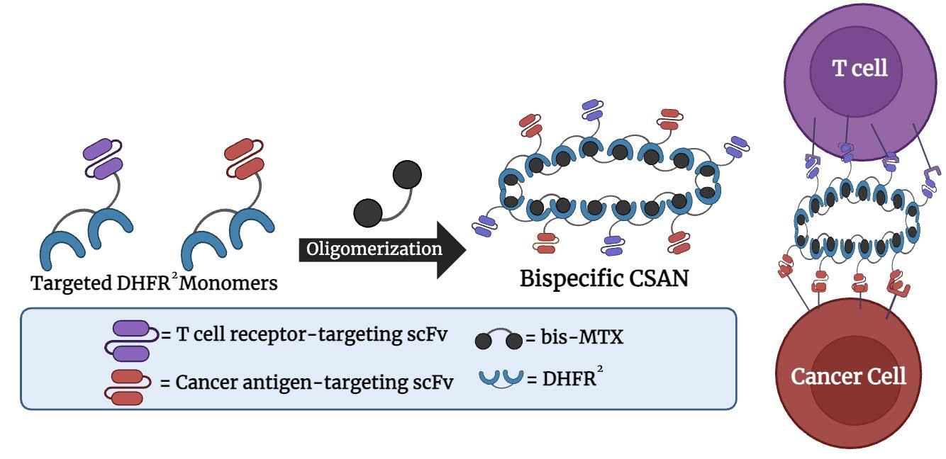
Figure 1. CSAN assembly from protein monomers to direct T cell killing of cancer cells. CSAN monomers assemble primarily into octameric rings with the addition of bis-MTX, which causes DHFR2 linking enzymes to oligomerize. CSANs created using both TCR-targeted monomers and cancer antigen-targeted monomers direct specific T cell killing of cancer cells Figure created by authors in BioRender
We used XL1-Blue E. coli to amplify a proprietary plasmid coding for ⍺TCR-1DDVHH CSAN monomers We inserted this plasmid into T7 SHuffle Express E. coli to express the protein The protein was collected and run on gel electrophoresis to confirm protein production and the protein’s water solubility. The protein was then purified using immobilized metal ion affinity chromatography (IMAC) and filtered. The protein production time was then compared to the known production time for the corresponding scFv
Bacterial Culture
All bacterial culture work was completed in a sterile environment. Competent E. coli XL1-blue (200249, Agilent Technologies) was used to expand and harvest a proprietary plasmid (Wagner, C., unpublished data) containing a gene conferring kanamycin resistance and the ⍺TCR-1DD-VHH gene driven by a T7 promoter T7 SHuffle Express (C3029J, New England Biolabs) bacteria were transformed with the plasmid and induced to express the protein of interest. Luria Broth (LB) medium was used for liquid cultures. Agar plates containing 1X kanamycin and LB were used for growth of single colonies.
Plasmid Expansion
An XL1-Blue stock containing the plasmid of interest was streaked onto agar plates, then incubated at 37°C overnight. A single colony was carefully removed with a pipette tip and dropped, along with the pipette tip, into a sterile, 100 mL Erlenmeyer flask containing 50 mL of LB and 50 µL of 1000x kanamycin The culture was placed on a shaking incubator at 250 rpm at 37°C overnight then stored at 4℃ .
The XL1-blue bacteria culture was lysed to harvest the plasmids using the Sigma-Aldrich Midiprep Kit (PLD35), according to the manufacturer’s directions 920 µL of the XL1-blue culture was combined with 80 µL of dimethylsulfoxide (DMSO) in a cryotube. The tube was frozen at -80℃ then allowed to thaw
Charlotte Vasicek and Michael Setterberg
The thawed mixture was centrifuged at 5000 xg, at 3℃ , and at an acceleration of nine for 10 minutes The cells were resuspended in 1 2 mL of Midiprep resuspension solution. 1.2 mL of Midiprep lysis solution was added to the cells The solution was neutralized with 1 6 mL of the Midiprep neutralization solution and mixed thoroughly before being centrifuged at 15,000 xg for 10 minutes at 3℃ at an acceleration of nine. Meanwhile, a GenElute Midiprep DNA binding column was placed in a 15 mL collection tube with 3 mL of Column Preparation Solution. This was centrifuged at 5000 xg for two minutes The flow-through was discarded and the lysate was loaded into the collection tube and centrifuged again at 5000 xg for two minutes The flow-through was discarded once again and the column was washed with a 3 mL mixture of ethanol and wash solution before being centrifuged at 5000 xg for five minutes The column was transferred to a new collection tube alongside 500 µL of the elution solution The tube was centrifuged at 5000 xg for five minutes The eluate concentration was analyzed before being stored at -20℃
50 µL of a 1 ng/µL plasmid solution was made by diluting a small amount of the isolated plasmid solution using the Midiprep elution buffer. 1 µL of the 1 ng/µL plasmid solution was mixed with thawed, competent E. coli T7 SHuffle Express cells These cells were then placed in a 42℃ water bath for 30 seconds before being transferred to an ice bucket for five minutes The cells were then added to 950 µL of Super Optimal Broth with catabolite repression medium (SOC; Sigma-Aldrich) before being placed in a 220 rpm shaking incubator for 60 minutes at 30℃ . 50 µL of this solution was spread on an LB and kanamycin plate and incubated at 30℃ overnight to form isolated colonies. A single colony was picked with a pipette tip, which was dropped into a sterile 100 mL Erlenmeyer flask containing 50 mL of LB and 50 µL of 1000x kanamycin. This was repeated to create an identical inoculated culture
The flasks were placed in a shaking incubator at 220 rpm at 30℃ overnight then stored at 4℃ The cultures were used to inoculate two 2L flasks each containing 1L of LB and kanamycin culture
Using a spectrophotometer, sterile LB was analyzed as a blank before the optical density of a 1 mL sample of the cell culture solution from one 2L flask was analyzed. It was previously determined that the maximum optimal optical density value the T7 SHuffle Express cells could reach before induction was 0.4 (Paul, D., personal communication, June 29, 2023) The culture flasks were incubated on a shaking incubator at 37℃ for two hours and the optical density measured each hour until it reached a value of 0 346 At this point, 120 mg of Isopropyl β-d-1-thiogalactopyranoside (IPTG) was added to two flasks containing 1 L of bacterial culture, then the flasks were placed on a shaking incubator for four hours at 37℃ to induce protein expression The solution was then stored at 4℃ overnight The bacterial culture solution was poured into four 250 mL centrifuge tubes to reach a total weight of 310 g per tube The tubes were centrifuged for 15 minutes at 4700 xg and 4℃ . The supernatant was discarded The remaining bacterial culture solution was divided between the centrifuge tubes and centrifuged at the same settings to create cell pellets Pellets were resuspended by forcefully pipetting 10 mL of 1x PBS into the centrifuge tube. The resuspended cell solution was pipetted into a 50 mL conical tube The centrifuge tube was then rinsed 3 more times using 10 mL of 1x PBS, and each rinse was pipetted into the conical tube, resulting in a total volume of 40 mL This was repeated for each cell pellet to transfer the cells out of the centrifuge tubes The conical tubes were balanced and centrifuged for 30 minutes at 3900 RPM at 4℃ . The supernatant was discarded and the pellets were stored at -80℃
100 µL Solulyse lysing solution was added to both a small, pre-prepared, pre-induction T7Shuffle Express cell pellet and a small, preprepared, post-induction T7-Shuffle Express cell pellet in a 1 5 mL Eppendorf (Epi) tube The cell pellets were thoroughly resuspended using a micropipette then sonicated at 22℃ for 45 minutes The lysed cells were centrifuged at 12,000 rpm for 5 minutes The soluble fraction of each sample was collected and placed in a 1.5 mL Epi tube The insoluble fractions were both thoroughly resuspended with 100 µL SoluLyse solution using a micropipette then sonicated for 30 minutes 28 µL of common mixture was prepared by heating a mixture of 8 µL Dithiothreitol (DTT) and 20 µL LDS Gel Loading Dye on a heat block for 5 minutes 7 µL of the common mixture was placed in four new 1.5 mL Epi tubes. 13 µL of solution was taken from both soluble fraction tubes and transferred to two of the Epi tubes containing the common mixtu re. 5 µL was taken from both insoluble fraction tubes and added to the two other Epi tubes alongside 8 µL of water The tubes were then heated in a tub of 80℃ water for 10 minutes before being centrifuged at 1000 xg for 30 seconds 10 µL of BenchMark protein ladder (Invitrogen) and 12 µL of each sample were loaded into separate wells in a pre-prepared electrophoresis gel (Invitrogen) The gel was run at 110V for about one hour then removed from the case and rinsed with deionized (DI) water The gel was placed in a 0 3% Coomassie Brilliant Blue solution which was diluted with DI water and heated in a microwave until bubbles appeared The heating was repeated until colored bands on the gel were visible. The dye was removed and replaced with DI water, and repeatedly heated to boiling to remove excess dye on the surface of the gel. Once most of the gel was destained, it was submerged in room temperature DI water alongside enough Kimwipes (Kimtech) to cover the sur face of the gel The gel was covered with plastic wrap and placed on a shaking plate overnight
Charlotte Vasicek and Michael Setterberg
The IMAC procedure to isolate ⍺TCR1DD-VHH from the cell lysate was was carried out at 4℃ An IMAC cobalt column was washed with enough 20% ethanol to fill the column. A 2 mL Epi tube was filled with the unfiltered lysate solution The other 38 mL of the lysate solution was run through the column, and the flowthrough was collected in two 20 mL Falcon tubes A sample was taken from each flowthrough Falcon tube and placed in 2 mL Epi tub es The column was eluted by adding ascending concentrations of imidazole to the column: 18 mL of 25 mM, 10 mL of 50 mM, 12 mL of 100 mM, 12 mL of 150 mM As each concentration of imidazole solution was run through the column, it was collected in 2 mL increments The samples of the initial lysate solution, the two flow through solutions, and 26 protein samples were then stored at 4℃ .
Gel electrophoresis was run using 12 µL samples from IMAC including the foll owing: the first and last collected samples for each different imidazole concentration, and intermediary samples in the middle of the first and last samples from each imidazole concentration were set aside Additional samples were added between the intermediary samples as available gel wells allowed The chosen samples from IMAC were each mixed with 7 µL of common mixture. Gel electrophoresis, staining and imaging was performed using the 12 µL IMAC samples, as previously described
IMAC samples that showed only single, prominent bands at 52 7 kD were selected for filtering. After combining the samples in a 50 mL conical tube, a 50 mL centrifuge filter tube was filled with 1x PBS at 4℃ to wet the filter The centrifuge filter prevented materials above 30 kDa from passing through The 1X PBS was removed from the filter and the upper chamber was filled with the protein solution. The filter tube was centrifuged at 3900 rpm, at 4℃ The
volume of protein solution remaining on top of the filter was not allowed to fall below the marked 5 mL line, preventing the protein from passing through the filter. More protein solution was added and centrifugation was repeated until all of the protein solution had been used and 5 mL of concentrated protein solution remained. The solution was rinsed by adding 1X PBS and centrifuging to a volume of 5 mL This was repeated four times to remove remaining imidazole The final centrifugation brought the solution to 4 mL The filtered, purified nanobody solution was stored at 4℃ .
Two 50 mL cultures were created to expand the plasmid coding for the ⍺TCR-1DD-VHH protein After plasmid isolation, one culture resulted in a plasmid concentration of 82.7 ng/µL, and the other resulted in a concentration of 93 1 ng/µL The resulting plasmid solutions were more than sufficient to inoculate the original 50 µL aliquot of T7 SHuffle E. coli used for protein expression
The two resulting liters of induced T7 SHuffle Express E coli bacteria culture solution were centrifuged to create four cell pellets that were lysed to obtain soluble and insoluble fractions for further analysis A small sample of pre-induction culture was also collected for comparison
The protein profile from soluble and insoluble fractions of lysed T7 SHuffle Express E coli was assessed by gel electrophoresis both pre- and post- induction by IPTG (Figure 2). The soluble, pre-induction sample showed multiple, relatively faint bands representing proteins of different weights. The insoluble, pre-induction sample showed very faint staining with no distinct bands The soluble, post-induction sample showed similar, but darker, bands as compared to the pre-induction soluble sample This sample
also had a very thick and dark band, at a weight of just higher than 50 kDa, that was not visible in either pre-induction sample The insoluble, post-induction sample also showed slightly darker bands than the pre-induction samples This sample also had a thicker and darker band at a weight of just over 50 kDa. The thickest band of protein visualized through gel electrophoresis was just over 50 kDa and it was in the soluble, post-induction sample.
from the imidazole concentration of 150 mM, there was not a visible band at this weight The two initial flow-through samples, as well as the first imidazole sample, showed high levels of protein present outside of the over-50 kDa weight Sample 5, taken in the middle of the imidazole concentration of 25 mM, showed very little protein outside of this weight, and the subsequent samples had little to no visible bands of protein outside of this weight.

Figure 2. Comparison of protein expression before and after induction in E coli The two samples on the left show the soluble and insoluble fractions from in T7 SHuffle Express E. coli containing the plasmid, before induction. The two samples on the right show the soluble and insoluble fractions from T7 SHuffle Express E coli containing the plasmid and after induction Figure by authors
The remaining half of the soluble fraction of a post-induction cell pellet was lysed, purified through IMAC, eluted using increasing concentrations of imidazole, and analyzed by gel electrophoresis (Figure 3). The first two flow-throughs from the IMAC and samples from the lowest imidazole concentration (25 mM) showed the thickest bands at a weight of just over 50 kDa, with the first imidazole sample showing the thickest band In the subsequent imidazole samples, going from the first, lowest to the last, highest imidazole concentration, this band decreased in thickness and visibility In the final samples, tubes collected 24th and 26th
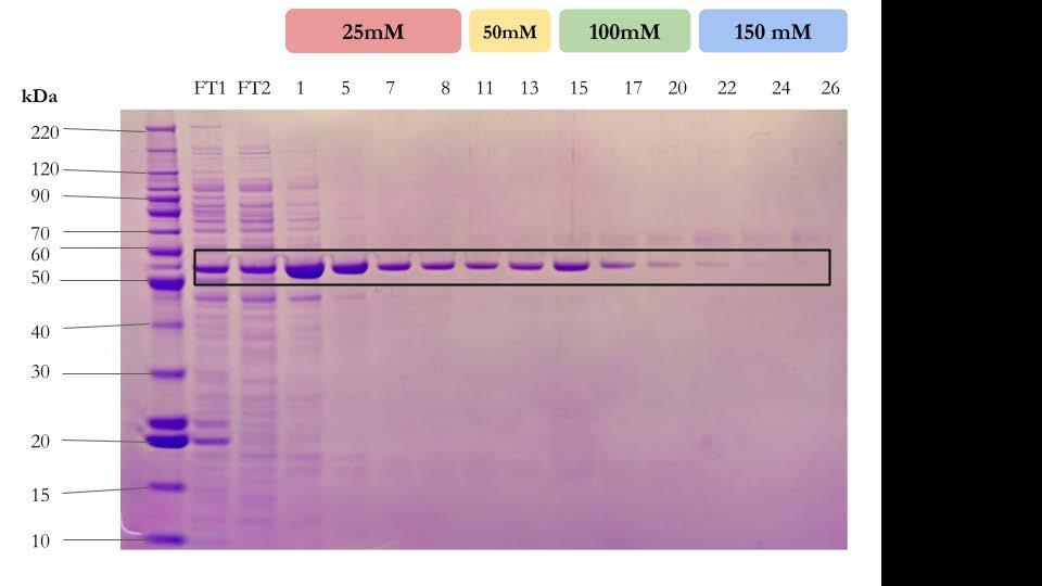
in presence after purification by e (half) FT1 and FT2 are the first hroughs after the cell lysate was run through the IMAC column The remaining samples show the result of eluting the protein from the IMAC column with increasing concentrations of imidazole, as labeled above the samples Figure by authors
The protein solution was filtered to remove the imidazole from IMAC Samples were chosen based on the gel electrophoresis results: Only samples with robust bands near 52 7 kDa, but little to no bands at any other weights, were chosen. The resulting concentrated protein solution had a volume of about 5 mL and gave a concentration of 0 712 mg/mL of protein This represented the yield from one cell pellet, created from 500 mL of bacterial culture
The work presented herein represents a proof-of-concept that nanobody-based CSAN monomers could provide a significant improvement in production time of CSANs, creating an easier path to the development of CSANs as a cancer therapy We produced
nanobody CSAN monomers containing a nanobody targeting the T cell receptor Expression and purification of ⍺TCR-1DD-VHH in E. coli took six days, and this production time could be realistically reduced to five days To begin with, running gel electrophoresis on the soluble and insoluble lysate fractions was not necessary after the first completion of the production process, since this step was only used to confirm that the protein was present and water soluble In addition, only a small amount of the expanded plasmid solution was used, meaning the same plasmid stock could be used multiple times In the future, the IMAC purification and gel electrophoresis of the IMAC samples could be completed in the same day, reducing the working days to just six This makes nanobodybased CSAN monomers much faster to produce than scFv-based monomers, which can take at least 20 working days to produce and purify (Dahlberg, D , personal communication, October 23, 2023). scFvs are insoluble, so they cannot be directly purified after the bacteria are lysed Instead, additional steps including solubilization and refolding are required before purification
Harvesting and lysing cells, collection of insoluble fraction/inclusion bodies
fi
Charlotte Vasicek and Michael Setterberg
(Table 1). scFv purification also requires multiple additional steps Because of this, scFv production not only requires more working days, but requires more active work. In comparison, most of the working days of nanobody production involve less work, such as bacterial culture work.
We measured a protein concentration of 0 712 mg/mL in 4 mL of purified protein solution, which was created from 500 mL of bacterial culture This was lower than expected, since the purification and filtration process for scFvs, when correctly completed, yields a solution of sufficient concentration for CSAN synthesis, while the concentration of the resulting nanobody solution was not sufficient for use (Paul, D , personal communication) Analysis by gel electrophoresis showed successful protein overexpression In addition, the purified protein solution had been concentrated to a lower volume than the samples used for gel electrophoresis
and lysing cells, collection of insoluble fraction/inclusion bodies
This suggests that the low concentration in the final, purified protein was due to error The final protein solution was stored overnight in the centrifuge filter and can still be absorbed into the filter over time This means that the low protein concentration was not necessarily due to flaws in the production process, but was likely caused by improper storage Although nanobodies are known to have similar specific binding capabilities compared to scFvs, the final ⍺TCR-1DD-VHH protein has not yet been tested for its capability to bind to the T cell receptor or evaluated for its ability to form into CSANs Thus, the next step will be to determine whether nanobody CSAN monomers form into rings with similar stability, binding affinity, and specificity to the currently used scFv-based CSANs
In the future, the ⍺TCR-1DD-VHH will be tested using size exclusion chromatography as well as flow cytometry to determine its ability to form CSANs and its binding affinity and specificity to the T cell receptor By confirming that the produced ⍺TCR-1DD-VHH protein is a functional CSAN monomer, we could bring nanobody CSANs into testing with T cell and tumor cell cultures and, eventually, into a novel and potentially-life saving cancer immunotherapy
We would like to thank Dr. Kati Kragtorp for advising us throughout this project Additionally, we would to thank Debasmita Paul, a graduate student in the Department of Medicinal Chemistry at the University of Minnesota, who taught us the scientific skills needed for this research and Dr. Carston R. Wagner, a professor and head of the Department of Medicinal Chemistry, who gave us the opportunity to work with the Wagner Lab.
Asaadi, Y , Jouneghani, F F , Janani, S , & Rahbarizadeh, F (2021) A comprehensive comparison between camelid nanobodies and single chain variable fragments Biomarker Research, 9(1), 87 https://doi org/10 1186/s40364-021-00332-6
Csizmar, C M , Petersburg, J R , Perry, T J , Rozumalski, L , Hackel, B. J., & Wagner, C. R. (2019). Multivalent Ligand Binding to Cell Membrane Antigens: Defining the Interplay of Affinity, Valency, and Expression Density Journal of the American Chemical Society, 141(1), 251–261 https://doi org/10 1021/jacs 8b09198
Hanahan, D , & Weinberg, R A (2011) Hallmarks of Cancer: The Next Generation Cell, 144(5), 646–674 https://doi.org/10.1016/j.cell.2011.02.013
Kilic, O , Matos De Souza, M R , Almotlak, A A , Wang, Y , Siegfried, J M , Distefano, M D , & Wagner, C R (2020) Anti-EGFR Fibronectin Bispecific Chemically Self-Assembling Nanorings (CSANs) Induce Potent T Cell-Mediated Antitumor Responses and Downregulation of EGFR Signaling and PD-1/PD-L1 Expression Journal of Medicinal Chemistry, 63(18), 10235–10245 https://doi org/10 1021/acs jmedchem 0c00489
Kumar, B V , Connors, T J , & Farber, D L (2018) Human T Cell Development, Localization, and Function throughout Life Immunity, 48(2), 202–213 https://doi org/10 1016/j immuni 2018 01 007
Li, Q , So, C R , Fegan, A , Cody, V , Sarikaya, M , Vallera, D A , & Wagner, C R (2010) Chemically Self-Assembled Antibody Nanorings (CSANs): Design and Characterization of an Anti-CD3 IgM Biomimetic Journal of the American Chemical Society, 132(48), 17247–17257 https://doi org/10 1021/ja107153a
Li, W , Wu, L , Huang, C , Liu, R , Li, Z , Liu, L , & Shan, B (2020) Challenges and strategies of clinical application of CAR-T therapy in the treatment of tumors a narrative review Annals of Translational Medicine, 8(17), 1093–1093 https://doi org/10 21037/atm-20-4502
Mews, E A , Beckmann, P , Patchava, M , Wang, Y , Largaespada, D A , & Wagner, C R (2022) Multivalent, Bispecific αB7-H3-αCD3 Chemically Self-Assembled Nanorings Direct Potent T Cell Responses against Medulloblastoma ACS Nano, 16(8), 12185–12201 https://doi org/10 1021/acsnano 2c02850
Miller, K D , Nogueira, L , Devasia, T , Mariotto, A B , Yabroff, K. R., Jemal, A., Kramer, J., & Siegel, R. L. (2022). Cancer treatment and survivorship statistics, 2022 CA: A Cancer Journal for Clinicians, 72(5), 409–436 https://doi org/10 3322/caac 21731
Siegel, R L , Miller, K D , Wagle, N S , & Jemal, A (2023) Cancer statistics, 2023 CA: A Cancer Journal for Clinicians, 73(1), 17–48 https://doi org/10 3322/caac 21763
Van De Donk, N W C J , & Zweegman, S (2023) T-cell-engaging bispecific antibodies in cancer. The Lancet, 402(10396), 142–158 https://doi org/10 1016/S0140-6736(23)00521-4
Vinay, D S , Ryan, E P , Pawelec, G , Talib, W H , Stagg, J , Elkord, E , Lichtor, T , Decker, W K , Whelan, R L , Kumara, H M C S , Signori, E , Honoki, K , Georgakilas, A G , Amin, A , Helferich, W G , Boosani, C S , Guha, G , Ciriolo, M R , Chen, S , Kwon, B S (2015) Immune evasion in cancer: Mechanistic basis and therapeutic strategies Seminars in Cancer Biology, 35, S185–S198 https://doi org/10 1016/j semcancer 2015 03 004
Wang, Y , Kilic, O , Csizmar, C M , Ashok, S , Hougland, J L , Distefano, M D , & Wagner, C R (n d ) Engineering reversible cell–cell interactions using enzymatically lipidated chemically self-assembled nanorings Chemical Science, 12(1), 331–340 https://doi org/10 1039/d0sc03194a
Elin Wellmann
Introduction
The U.S is the world’s largest contributor to plastic pollution, generating 42 million metric tons of plastic a year (Lai, 2023). A majority of the plastic released into the environment breaks down into smaller fragments called microplastics. Microplastics have been found almost everywhere, even in the most remote ocean l ocations and Antarctica (Magazine & Osborne, n.d.). Not only can this plastic waste affect the environment, but it can make its way into humans as well Humans ingest five grams of microplastics each week, and the average human ingests about 44 pounds of microplastic in their lifetime (Lai, 2023) However, the consequences of ingesting this much microplastic are unknown.
Microplastics are defined as fragments that have a diameter less than 5 mm Sources of microplastics are usually categorized into primary and secondary Primary sources are intentionally-made microplastics that are used in products such as cleaning abrasives, microfibers in clothes, or plastic powder (Lamichhane et al , 2023) Secondary sources are larger plastic items, including plastic water bottles, nets, or bags, that, over time, have undergone fragmentation, weathering, biodegradation, or hydrolysis to become microplastics (Gewert et al , 2015) Microplastics have a variety of chemical make ups, as there are many different polymers used in creating plastics. In 2020, the two most highly-demanded plastic polymers were polypropylene and polyethylene, both of which are used to make single-use food packaging and wrappers (Plastics-the-Facts2021-Web-Final Pdf, n d )
Microplastics can move through the environment and through food chains Due to the small size

and light weight of microplastics, they are easily transported by wind and water However, microplastics are also transported by organisms For example, worms aid the transport of microplastics from surface level soil to deep level soil through burrowing (Huerta Lwanga et al., 2017). In addition, microplastic uptake by primary consumers is the starting point for bioaccumulation Microplastics readily bioaccumulate, meaning that they can move through the food chain to reach especially high concentrations in top-order predators (Farrell & Nelson, 2013). Thus, microplastics pose a potential threat to all organisms, worldwide
One way microplastics could harm organisms is by interfering with animals' intake of nutrition. In bees, microplastic exposure significantly decreased feeding rate and body size, although it did not directly affect their survival rate (Al Naggar et al., 2023). Another major concern regarding microplastics is their ability to adhere to other chemicals. Due to micr oplastics' large surface area and hydrophobic nature, other toxins, including pesticides and organic pollutants, can be easily adsorbed onto the surface of microplastics (Rochman et al., 2013). Over 50% of plastics are known to have dangerous additives and chemical byproducts (Rochman et al., 2013). Polyethylene, one of the most common plastics, has the greatest affinity for organic contaminants compared to other common plastics.
The majority of research on micropla stics in ecosystems has been in ocean environments, with much less research done on microplastics in terrestrial environments (Rillig, 2012) Since microplastics enter the food chain through primary consumers, one major concern is how microplastics are affecting these primary consumers. The few studies on how
microplastics are harming terrestrial primary consumers provide mixed results In mosquitoes, exposure to microplastics did not significantly affect survival to adulthood (Al-Jaibachi et al., 2019) On the other hand, long-fibered microplastic reduced survival rates and reproduction of earthworms (Selonen et al., 2020) Clearly, more research is needed to determine how microplastics are affecting terrestrial primary consumers.
To address this gap, I reared cabbage white butterflies (Pieris rapae) in a microplastics dose-response experiment. Cabbage white butterflies are an invasive species with a short lifespan that is ideal for experimentation (Webb & Shelton, 1988). I collected wild, female, cabbage white butterflies and induced them to lay eggs in an enclosure in order to collect newly-emerged larvae. Newly emerged larvae were transferred to diets consisting of 0%, 0 5%, 1%, 2%, 4%, or 8% polyethylene (PE) microplastic by weight. The larvae stayed on these diets until they became adult cabbage white butterflies Once they emerged, the date and butterfly number were noted to collect survival data. One forewing was removed and measured as an indication of body size Female butterflies were dissected for egg count as a measure of fecundity. Survival was significantly affected by diet type Survival rates of the butterflies exposed to 1% and 4% microplastic diets were significantly lower relative to the control diet Development time, wing area, and fecundity were not significantly affected by diet type.
butterflies
Cabbage white butterflies (Pieris rapae) were collected from various sites around the Twin Cities urban area After catching them with a net, the butterflies were slid into a parchment envelope and placed on an ice pack, causing them to enter a dormant state Specimens were stored at 6℃ until ready to use for egg collection
To set up for egg collection I first collected wild female Pieris rapae Then, I made a 10% honey (Kirkland Organic Raw Honey) solution in water. Three small sponges were placed in three petri dishes and just enough honey water was added to cover the bottom of the petri dishes Then, three tubes were filled with water and capped with a cap that had a small hole in the top Two to three stems of kale, harvested from a pesticide-free garden, were inserted through the hole into the tube The honey water petri dishes and kale stems were evenly spaced in the cage Next, the female Pieris rapae were taken out of their envelopes and introduced to either the sponge or the kale Once all of the butterflies were in the cage, the cage was placed on a windowsill, in direct sunlight, to encourage egg-laying (Figure 1) The next day the kale leaves were inspected for eggs. If there were eggs, the kale would be removed from the enclosure The number of eggs laid would be recorded, and the kale with the eggs would be enclosed in a plastic container and placed in a 24℃ li t h b Thi ess was r t.
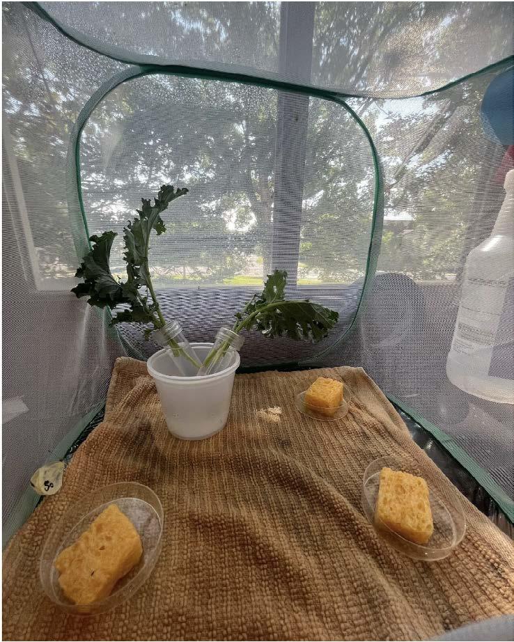
lection.
Cabbage white larvae were reared on artificial diets with varying levels of microplastics The artificial diet recipe was based on an established protocol previously demonstrated to raise healthy cabbage white butterflies in captivity (E Snell-Rood, unpublished observations) The base
Elin Wellmann
diet was 31.9% wheat germ (Frontier Agriculture Sciences), 9 6% cabbage flour (Frontier Agricultural Sciences), 17 2% casein (Frontier Agriculture Sciences), 15.3% sugar (Target brand), 5 7% Wesson salt mix (Frontier Agriculture Sciences), 7 7% yeast (Frontier Agricultural Sciences), 2.3% cholesterol (Frontier Agriculture Sciences), 6 7% vitamin mix (Frontier Agriculture Sciences), 0 48% methyl paraben (Frontier Agriculture Sciences), 0 96% sorbic acid (Frontier Agriculture Sciences), 1 9% ascorbic acid (Frontier Agriculture Sciences), and 0.11% streptomycin (Sigma) The base diet was stored at 4°C until ready for use Polyethylene powder (1000 mesh; Magerial Sciences) was used as the microplastic. Cellulose was used as the control for polyethylene 9 6% of the diet by mass contained either cellulose or a cellulose/ polyethylene mixture Increasing concentrations of polyethylene in cellulose were added to create diets that were 0.5%, 1%, 2%, 4%, and 8% polyethylene by mass Organic flaxseed oil (Puritan’s Pride) was then added to a final concentration of 3.2% of the entire diet. Finally I mixed 0 19 grams of diet per ml of a 10% agar and water solution I poured the diets into 5 oz plastic cups so the diet was just covering the bottom The cups were stored at 6℃ until ready for use
Larvae transfer
Once caterpillars emerged from the eggs, they were randomly transferred to the microplastic diets. Kale leaves were removed from the 24℃ climate chamber and inspected for larvae A small paintbrush was cleaned using a 10% bleach solution in water. I used the paint brush and gently lifted the larvae off of the kale into a diet cup I repeated this process until there were a maximum of three larvae in each diet cup. I poked holes in the top of the diet cups for airflow and labeled them with the number of larvae in that cup. I recorded the individual number, diet type, number of larvae in the cup, cup number, the date the eggs were collected, date of transfer, and host plant. The cups were
kept in a 24℃ climate chamber until the larvae emerged as butterflies
Measurements
I tracked larval development time (time from egg to adult) and survival rate of caterpillars on each of the diets When the butterflies emerged they were kept in a mesh enclosure with honey water for two days while their wings hardened. Two days after emerging, they were sacrificed for fitnes s measurements. Each butterfly was placed in an envelope and kept at 6℃ for roughly 30 minutes
Fecundity of the cabbage white butterflies was measured through egg count. The butterflies were first separated by sex, to identify the females. I filled a shallow petri dish with 1x phosphate-buffered saline (PBS; Quality Biological) solution I took a butterfly out of the envelope it was stored in using delicate forceps. Then, using small scissors, I cut off the abdomen where it connected to the thorax The abdomen was placed in the petri dish and viewed under a dissecting microscope at 10x and 20x magnification Using forceps and microscissors, I made an incision horizontally along the abdomen. Then, I pulled open the abdomen at the incision and removed the insides I located the ovaries and unraveled them. The number of mature eggs was recorded. Mature eggs are distinguished from immature eggs by being fully-yolked, and having striations on their surface (Kingsolver, 2000).
To measure wing size, a forewing was removed from each butterfly Wings were photographed inside side up in a light box with a ruler for scale The perimeter, length, and area of each wing were measured using Image J (Schneider et al., 2012).
JMP statistical software (JMP, n d ) was used to analyze data. A chi-squared test was performed on survival data and both diet type and survival status were treated as categorical variables ANOVA tests were performed to compare the means of the measurement data
When a butterfly emerged, their unique identification number, diet, and emergence date were recorded to calculate the survival rate of cabbage white butterflies for each diet. Survival was statistically significantly affected by diet type (p < 0.0001; Figure 2). Survival was statistically significantly lower than the control diet on the 1% (p < 0 0001) and 4% (p < 0 0001) microplastic diets.
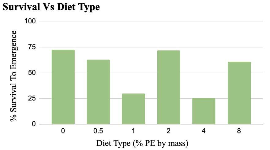
Figure 2. Survival rate of cabbage white butterflies raised on microplastic diets Survival was significantly affected by diet (Χ2 = 41.47, p < 0.0001, 0% n = 47, 0.5% n = 43, 1% n = 44, 2% n = 46, 4% n = 47, 8% n = 46) type.
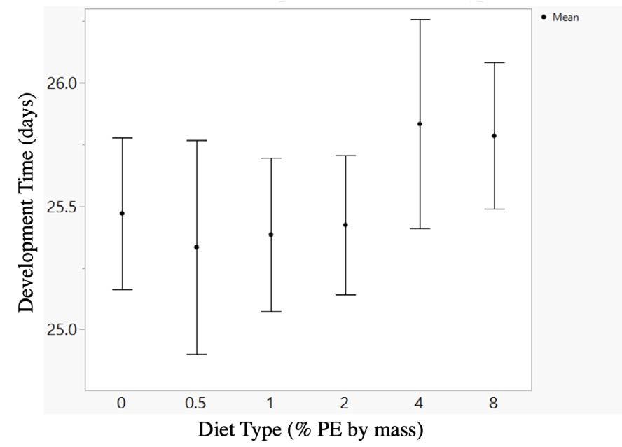
Figure 3. Mean Development Time with standard error of cabbage white butterflies raised on 0%,0 5%,1%,2%,4%, and 8% PE diets There was no significant effect of microplastics on the development time (F = 0 31, p = 0 91, 0% n = 34, 0 5% n = 27, 1% n = 13, 2% n = 33, 4% n = 12, 8% n = 28 ).
Effect of Diet Type on Mean Development Time
The time between the eggs laid and the emergence of the butterfly was used as development time Though the mean development time of 4% and 8% diets were longer compared to the other diets, the differences were not statistically significant (ANOVA, p = 0.9058; Figure 3).
Effect of diet type on mean wing area
The forewings of all butterflies who survived to adulthood were measured using ImageJ to calculate the area of the wing. The wing area data was separated by sex because male cabbag e white butterflies are, on average, larger than females. Within each sex group there were no statistically significant differences in mean wing area between the diet types (Figure 4).
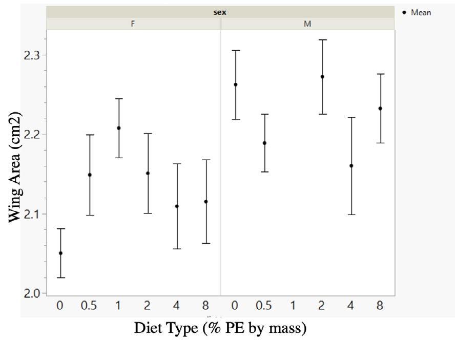
Figure 4. Mean wing area with standard error of cabbage white butterflies exposed to microplastic diets. This graph separates male butterflies (on the right) from females (on the left; Female: 0%: n = 18; 0 5%: n = 14; 1%: n = 13; 2%: n = 19; 4%: n = 6; 8%: n = 13, Male: 0%: n = 15; 0 5%: n = 13; 1%: n = 0; 2%: n = 14; 4%: n = 6; 8%: n = 15) There was no significant difference of wing area within each sex (Diet type: F = 1.14, p = 0.35).
Effect of diet type on number of mature eggs
All of the female butterflies were dissected and their mature eggs were counted There were no significant differences in the number of mature eggs between the diets (ANOVA analysis, p = 0 79, Mated status: F= 8 63, p = 0 007, mated > unmated; Figure 5).
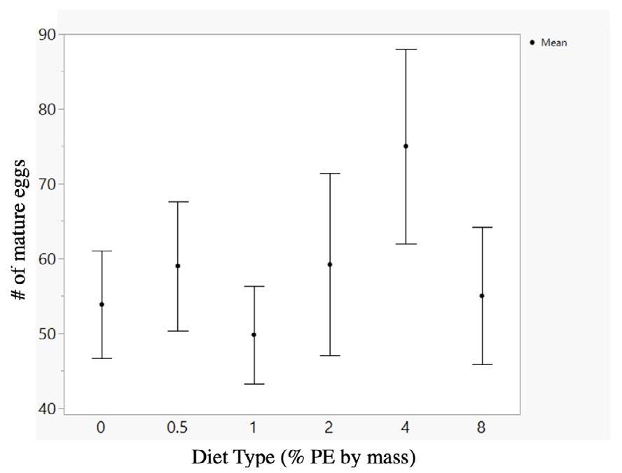
Figure 5. Mean number of mature eggs, with standard error, in female cabbage white butterflies for each diet Graph shows raw means and SE Model controls for mated status There was no significant difference in the number of mature eggs between the diets (F = 0.47, p = 0.79).
Diet type significantly affected the survival rate of cabbage white butterflies. However, the variation in survival rate was unexpected It was expected that the survival rate of the butterflies would decrease as the percent polyethylene in the diets increased However, only the survival rates of the 1% and 4% microplastic diets were significantly lower than the control. Additionally, fecundity, wing area, and development time were not significantly affected by diet type. These measurements could be influenced by survivorship bias if the butterflies that were most strongly affected by the microplastic diets did not survive to adulthood. If that were the case, I would expect to see higher measurements in the groups with lower survivorship. However, there are no noticeable trends to clearly indicate this
Limitations and future work
Pure polyethylene powder was used as the microplastic source in this study, however, this is not representative of the microplastics cabbage white butterflies would find in the wild. A majority of environmental microplastics are a combination of polymers and have additives. I originally attempted to conduct this experiment with ground astroturf, synthetic rubber that is
very similar to tire crumbs that are often used on artificial athletic fields The diets with the astroturf became overgrown with bacteria, and had to be thrown out. Thus, a next step in this research is finding an alternative microplastic source that is more representative of environmental microplastics and measuring its effect on cabbage white butterflies Additionally, it is unknown whether the microplastic levels used in this study were representative of the levels cabbage white larvae are exposed to in the environment There is currently research in progress focused on analyzing the amounts of microplastics on common plants in urban, semi-urban, and rural areas (E Snell-Rood, personal communication). This information will be used to create a more precise dose-response experiment Finally, research is being conducted to measure the excretion rate of the butterflies on the different microplastic diets (E Snell-Rood, personal communication) It is possible the butterflies exposed to higher levels of microplastic responded with increased excretion to eliminate the microplastics and thus had to ingest more food to stay full. Although there is still much we do not know about the risks microplastics pose, this research provides an important step towards a better understanding of how microplastics could be affecting organisms, ecosystems and, eventually, human health
I would like to thank Dr. Emilie Snell-Rood, a Professor at the University of Minnesota in the Department of Ecology, Evolution, and Behavior, for hosting me in her lab this summer and all her mentorship throughout the research process I would also like to thank the other members of the Snell-Rood lab for answering all my questions, and their support Finally, I would like to thank Dr Kati Kragtorp for her guidance and help in creating my paper and project.
Al Naggar, Y , Sayes, C M , Collom, C , Ayorinde, T , Qi, S , El-Seedi, H R , Paxton, R J , & Wang, K (2023) Chronic Exposure to Polystyrene Microplastic Fragments Has No Effect on Honey Bee Survival, but Reduces Feeding Rate and Body Weight Toxics, 11(2), Article 2 https://doi org/10 3390/toxics11020100
Al-Jaibachi, R , Cuthbert, R N , & Callaghan, A (2019) Examining effects of ontogenic microplastic transference on Culex mosquito mortality and adult weight Science of The Total Environment, 651, 871–876
https://doi org/10 1016/j scitotenv 2018 09 236
Farrell, P , & Nelson, K (2013) Trophic level transfer of microplastic: Mytilus edulis (L ) to Carcinus maenas (L ) Environmental Pollution, 177, 1–3 https://doi org/10 1016/j envpol 2013 01 046
Gewert, B , Plassmann, M M , & MacLeod, M (2015) Pathways for degradation of plastic polymers floating in the marine environment Environmental Science: Processes & Impacts, 17(9), 1513–1521 https://doi org/10 1039/C5EM00207A
Huerta Lwanga, E , Gertsen, H , Gooren, H , Peters, P , Salánki, T , van der Ploeg, M , Besseling, E , Koelmans, A A , & Geissen, V (2017). Incorporation of microplastics from litter into burrows of Lumbricus terrestris Environmental Pollution, 220, 523–531 https://doi org/10 1016/j envpol 2016 09 096
JMP (n d ) [Computer software] SAS Institute Inc
Kingsolver, J G (2000) Feeding, Growth, and the Thermal Environment of Cabbage White Caterpillars, Pieris rapae L Physiological and Biochemical Zoology: Ecological and Evolutionary Approaches, 73(5), 621–628. https://doi org/10 1086/317758
Lai, O (2023, May 30) 8 Shocking Plastic Pollution Statistics to Know About Earth Org https://earth org/plastic-pollution-statistics/
Lamichhane, G , Acharya, A , Marahatha, R , Modi, B , Paudel, R , Adhikari, A., Raut, B. K., Aryal, S., & Parajuli, N. (2023). Microplastics in environment: Global concern, challenges, and controlling measures International Journal of Environmental Science and Technology, 20(4), 4673 https://doi org/10 1007/s13762-022-04261-1
Magazine, S , & Osborne, M (n d ) In a First, Microplastics Are Found in Fresh Antarctic Snow Smithsonian Magazine Retrieved November 12, 2023, from https://www.smithsonianmag.com/smart-news/in-a-first-microplast ics-are-found-in-fresh-antarctic-snow-180980264/
Plastics-the-Facts-2021-web-final pdf (n d ) Retrieved November 12, 2023, from https://plasticseurope org/wp-content/uploads/2021/12/Plastics-theFacts-2021-web-final pdf
Rillig, M. C. (2012). Microplastic in Terrestrial Ecosystems and the Soil? Environmental Science & Technology, 46(12), 6453–6454 https://doi org/10 1021/es302011r
Rochman, C M , Hoh, E , Kurobe, T , & Teh, S J (2013) Ingested plastic transfers hazardous chemicals to fish and induces hepatic stress Scientific Reports, 3(1), 3263 https://doi org/10 1038/srep03263
Schneider, C. A., Rasband, W. S., & Eliceiri, K. W. (2012). NIH Image to ImageJ: 25 years of image analysis Nature Methods, 9(7), Article 7 https://doi org/10 1038/nmeth 2089
Selonen, S , Dolar, A , Jemec Kokalj, A , Skalar, T , Parramon Dolcet, L , Hurley, R , & van Gestel, C A M (2020) Exploring the impacts of plastics in soil – The effects of polyester textile
fibers on soil invertebrates Science of The Total Environment, 700, 134451. https://doi.org/10.1016/j.scitotenv.2019.134451
Webb, S , & Shelton, A (1988) Laboratory rearing of the imported cabbageworm New York’s Food Life Sci Bull , 122
Breck School
123 Ottawa Avenue North Golden Valley, MN 55422
breckschool.org | 763.381.8100