
Filippo Nicolai

Using Stellar Remnants to Understand
How Often Massive Stars Form Planets
Abstract
White dwarfs are dead, burnt cores of stars whose outer layers have been lost. They are characterized by their stellar spectra, whose absorption lines yield the elements making up their atmospheres. The most common types are white dwarfs showing Hydrogen lines, Helium lines, and no lines (continuum). A few show metal lines in their spectra. Because of the high surface gravity of white dwarfs, any metals already present on their surfaces very quickly sink below the atmosphere. Therefore, the most common way to see metal lines on a white dwarf is from metal pollution from external sources like planets. Thus, white dwarfs that show metal lines indicate that their ancestor star had planets orbiting it. The purpose of my study was to analyze the mass distribution of metal-polluted white dwarfs compared to other white dwarfs and use it to draw conclusions about the presence of remnant planetary systems around massive stars. My results were then compared to a recent study from Boston University graduate
student Lou Baya Ould Rouis, which shows a significant decrease in metal-polluted white dwarfs at higher masses compared to other white dwarfs. In my study, the white dwarfs were matched based on temperature and magnitude, and their mass distributions were then contrasted. Even though the focus was on massive ( ≥ 0.8 M☉) white dwarfs, I used masses of 0.6 M☉ and greater to avoid skewed results. I found that, while there were fewer metal-polluted white dwarfs on the massive end, the difference was about 4 times smaller than that found in Ould Rouis’ research.
Introduction
The creation of a star begins when gas and dust particles clump together. Over time, the cloud becomes bigger and heaver, spins faster, and heats up. A star is born when its core heats up so much that it can fuse two Hydrogen (H) atoms into a Helium (He) atom (NASA).
During a star’s lifetime, there are two major forces at play: gravity and radiation pressure. Gravity pulls inward and tries to crush the star into itself. Radiation pressure pushes outward, countering gravity. A star’s radiation pressure is caused by the hot gas inside of it. This gas is maintained hot by the enormous amounts of energy released by the fusion of H atoms into He atoms (Kawaler et al. 2000).
When the forces of radiation pressure and gravity balance each other, the star is in its main-sequence phase. However, after billions of years, the star eventually runs out of H atoms to fuse.
Once this occurs, fusion inside the core stops, which marks the beginning of the end for a star’s life (Kawaler et al. 2000).
As fusion stops, gravity wins, contracting the core. What happens next differs from star to star depending on its mass. Some stars explode into supernovae and turn into black holes. Others form neutron stars. However, the ones that this study focuses on are stars that begin their lives with a mass less than around 8 M☉ (M☉ is the unit in terms of solar masses). These stars are not quite massive enough for the processes just mentioned, so they instead form white dwarfs (Dobrijevic et al. 2022).
In these stars, the energy released from the contraction of the core causes the outer layers of the star to expand to hundreds of times their original radius. The star enters its red giant phase (Kawaler et al. 2000).
Because the core has contracted, there is now even more energy inside it. Indeed, there is so much pressure that the star
starts to fuse He atoms into heavier elements, like Carbon (C). Eventually, however, the He stores run out as well, and the core contracts once again. This time, the energy from the contraction is such that the star’s outer envelope is released into a stellar nebula (fig. 1). The remaining exposed core in the middle of the nebula is a white dwarf (Kawaler et al. 2000).
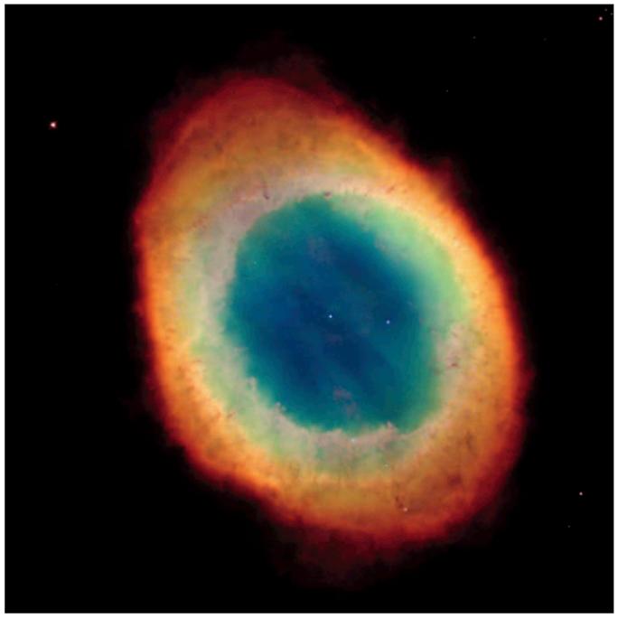
Figure 1. Stellar nebula caused by the ejection of a star’s outer layer. Remaining white dot in the middle is the star’s dead core – a white dwarf. Hubble Heritage Team (AURA/STScI/NASA).
In the universe, different types of white dwarfs can be found. White dwarfs are identified by the absorption lines in their stellar spectra.
The spectrum of a white dwarf is the light emitted by it separated into different wavelengths. When a photon of light hits an electron in an atom, that electron may gain enough energy to get ‘excited’ and jump to the next energy level. However, an electron can only jump whole energy levels, not portions of them. Therefore, it requires a very specific amount of energy to make the jump. If a photon of that energy hits it, the electron gets excited and absorbs the photon, creating a dip in the light spectrum–an absorption line (Webb Space Telescope, 2022). This process happening in a H atom is shown in the diagrams in Figure 2.
Absorption lines are used in two different ways when characterizing a white dwarf. One is to actually determine whether a light source is a white dwarf. When the core of a star contracts, it
retains its mass but shrinks down to relatively small sizes, becoming extremely dense. For perspective, an average white dwarf can have a mass similar to that of the Sun but a radius close to that of the Earth. This means that a teaspoon of a white dwarf would weigh more than an average elephant!
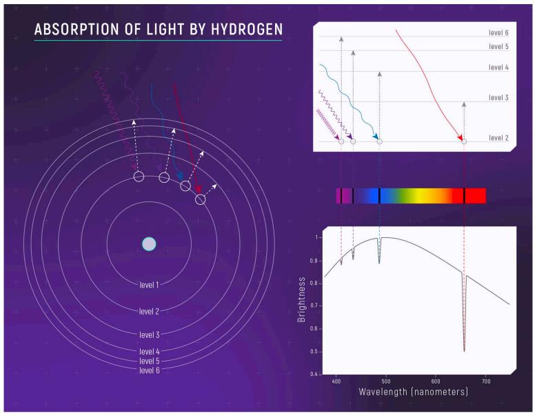
Figure 2. Diagram of electrons in a Hydrogen atom absorbing photons of light of different energies. NASA, ESA, and L. Hustak (STScI).
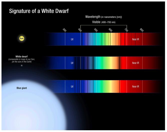
Figure 3. Diagram of absorption lines for different celestial bodies, showing very wide absorption lines for white dwarfs. NASA, ESA, and A. Feild and J. Kalirai (STScI).
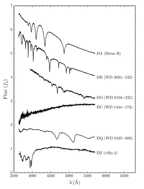
Figure 4. Light spectrum from different types of white dwarfs (DA: H, DB: He, DO: C/O, DC: continuum, DQ: C, DZ: metals). Each dip in the spectra is an absorption line. Saumon, D., et al. 2022.
This density greatly increases the gravity at the surface of a dwarf. The force of gravity is directly proportional to the mass of the dwarf and inversely proportional to its radius. As explained above, the radius of these stellar remnants is usually quite small, while the mass is very high. Therefore, a white dwarf’s surface gravity is extremely strong, with a log g value of about 8 (where g is the acceleration due to gravity at the surface of a white dwarf in units of cm ⋅ s 2) (Dufour et al. 2010). For reference, the log g value for the Sun is 4!
The extremely strong gravity, in turn, greatly increases the pressure on the surface of the dwarf, perturbing the energy levels of the atoms in atmosphere and broadening their absorption lines. This is clearly displayed in Figure 3, where the dips in the spectrum much wider for the white dwarf. This is also visible in Figure 4, which shows actual spectra from different white dwarfs with very wide absorption lines. Since white dwarf lines are
broadened in this way, they are a telltale sign of these stellar remnants.
Absorption lines are also used by scientists to understand which elements make up a white dwarf’s atmosphere. For each element, the electrons in its atoms require photons of different energies to get excited. Therefore, every element has its own set of absorption lines which they can be identified from. When light is emitted from the white dwarf, the elements in its atmosphere interact with the outgoing photons and create absorption lines.
The most common white dwarf is a DA, which shows H lines–hence indicating an H-dominated atmosphere. Another type is DBs, which show He lines. DCs show no lines. They often have a mixed atmosphere containing both H and He or one that is dominated by either element. Their spectra don’t show lines because their atmospheres are too cold for photons to interact with H or He atoms. There are also DZs, which show heavier elements
(which I will generally refer to as metals) in their atmospheres.
DAZs and DBZs are subtypes of DZs which also show H or He lines, respectively. There are other white dwarf types, but they are not relevant for the purposes of this study.
As explained before, the gravity at the surface of these dead stellar cores is extremely high. Therefore, any metals present on the surfaces of white dwarfs sink below the atmosphere in just a matter of days and should, thus, be undetectable in the dwarf’s light spectra. So, how is it possible to see metals in DZs’ atmospheres?
The answer is not found in the white dwarfs themselves but in the objects around them. Specifically, the metal in their atmospheres mostly comes from metal pollution from outside sources. The metal present in the spectra is not intrinsically the white dwarf’s but is being accreted from other astronomical bodies, especially planets (Ould Rouis 2024). When scientists find
metal lines in a white dwarf’s spectra, those metals are in the process of being accreted by the white dwarf.
Since the metal shown by DZs is being accreted from planetary systems, these white dwarfs indirectly indicate that there are planets orbiting around them. Consequently, they show that these planets also orbited their predecessor star. Hence, DZ white dwarfs can give a lot of information regarding the kinds of stars that form planets.
During early 2023, Boston University (BU) graduate student and BU White Dwarf group (BUWD) member Lou Baya Ould Rouis conducted research on massive (masses greater than 0.8 M☉) white dwarfs using ultraviolet (UV) observations from the Hubble Space Telescope (HST). The overarching goal of her research was to understand if more massive white dwarfs show fewer remnant planetary systems. To do this, she compared the mass distribution of DAZs to DAs. It is important to note that, in
her sample, the surface temperatures of the white dwarfs were greater than 15,000K.
Ould Rouis found around 7 times fewer DZs in the massive end compared to other white dwarfs. This discrepancy could be an indication that massive (masses over 4 M☉) stars do not form or host planets. A crucial thing to mention about the UV sample is that there may be an observational bias. To understand this bias, it is first important to mention that metal accretion is not the only way for white dwarfs to show metals in their atmospheres. Two other processes are relevant for this bias: convection and radiative levitation (Ould Rouis 2024).
Subsurface convection mixes the material inside a star and dredges up metals from deeper in the white dwarf into its atmosphere. Therefore, it is impossible to know if the metal lines seen from white dwarfs are from metal pollution or from convection. However, this process only occurs on white dwarfs
cooler than about 15,000K. Therefore, my study was affected by convection but the UV sample was not. That being said, there was no need to account for it in my research as it should affect the sample more or less uniformly (Ould Rouis 2024).
There is another way for metals to appear in the atmosphere–radiative levitation. In this process, the radiation caused by the white dwarf’s high surface temperature counteracts gravitational settling and keeps accreted metals in the white dwarfs’ atmospheres for longer than expected. Since the white dwarfs must be hot for radiative levitation to happen, only those with an effective surface temperature higher than about 20,000K experience it. Therefore, no white dwarfs in my study were affected, but most of those in the UV sample were. Importantly, the effects of radiative levitation are much weaker on more massive dwarfs, creating a bias. While less massive white dwarfs would still show accreted metals, due to the slowing of the time it takes for metals to sink, they may show older metals that, were they
accreted by a massive dwarf, would already have sunk too deep to be observed. This could have resulted in more drastic differences between low- and high-mass white dwarfs in Ould Rouis’ results (Ould Rouis 2024).
The purpose of this study was to test the results from the UV sample and see if they also apply for white dwarfs with surface temperatures lower than 15,000K. Different samples of the same size separated by white dwarf type were created, their mass distributions analyzed, and results drawn. Then, a comparison was made to Ould Rouis’ findings.
Furthermore, since the possible bias in the UV sample was caused by the high surface temperatures of the selected white dwarfs, by using cooler white dwarfs my study also aims to test the presence of this bias and help form better conclusions.
The study was conducted at BUWD, and I was advised by BU Assistant Professor and BUWD PI, JJ Hermes.
Methods
The data used in this study were acquired from multiple existing white dwarf databases. Three datasets were used, and different pieces of information were taken from each list. The data manipulation process explained in this section was done on Python.
Two of the databases came from Nicola Pietro Gentile Fusillo’s catalogues from Gaia Early Data Release 3 (EDR3) (Gaia is a European Space Agency (ESA) mission) (2021). Data were also taken from the Montreal White Dwarf Database (MWDD) (Dufour et al. 2016).
The white dwarfs’ mass, magnitude, and temperature values were taken from the main database in Gentile Fusillo’s study. Meanwhile, the type of white dwarf (DA, DC, etc.) was determined from another of Gentile Fusillo’s catalogues, which
contains Sloan Digital Sky Survey (SDSS) spectral classification, as well as the MWDD.
All three of these datasets contain a variable to identify each white dwarfs. These variables were used to correctly match the databases for every star, with values from each dataset combining into one row per star. The white dwarfs that were not overlapping across the databases were removed from the final list.
Once the dataset was finalized, two subsets were created, one containing DAs and the other containing DZs, DAZs, and DBZs (D*Zs).
Before further explaining the process of this research, it is important to mention that the mass and radius values in Gentile Fusillo’s catalogues were determined by using two independent stellar parameters (temperature and log g) in different models for different types of white dwarfs.
Since the DA subset was much larger than the D*Z subset, I had to modify it so it contained the same number of white dwarfs.
I did this by matching apparent magnitude (G) (the brightness of a white dwarf observed on Earth) and effective temperature (Teff) values across white dwarfs. Magnitude was chosen as a value of comparison because a similar magnitude would help avoid possible observational biases, since faint stars are harder to detect and analyze. Meanwhile, temperature was picked as a similar temperature distribution would allow for more alike white dwarfs across datasets and a more even comparison.
Before matching, I removed any white dwarfs with a missing magnitude or temperature parameter.
Next, I had to assign the right temperature and mass values to each white dwarf. In Gentile Fusillo’s main catalogue, there were three variables for temperature and mass per white dwarf. Each variable either ended with H, being most accurate for H-
dominated atmospheres; He, being most accurate for Hedominated atmospheres; and _mixed for white dwarfs with a mixed (H and He) atmosphere.
Since all DAs have H-dominant atmospheres, I assigned them the temperature and mass variables ending in H.
For D*Zs, the process was slightly more complicated, as they can contain different elements in their atmospheres. I first assigned DZs the variables ending in He. However, it was later determined that using the values for mixed atmospheres would yield better results, so those were used for the final results (Gentile Fusillo et al. 2021). DAZs are dominated by H and DBZs are dominated by He, so I used the H and He variables, respectively, for these two types of white dwarfs.
Due to this study’s focus on white dwarfs with surface temperatures lower than 15,000K, I then proceeded to remove any white dwarfs with surface temperatures higher than that.
Finally, I removed any white dwarfs with a missing mass value. I also removed any white dwarfs less than 0.6 M☉ because of the implication of such a light mass. A star’s lifetime is inversely proportional to its mass. This is due to the fact that, to not collapse under their greater weight, more massive stars burn through their H fuel at a much faster rate than less massive ones. Therefore, they run out of H to fuse more quickly (NASA).
Because of the finite age of the universe, it is rare that a star producing a white dwarf of mass lighter than 0.6 M☉ has already died. Therefore, while they do exist, most white dwarfs this light have likely lost some of their mass to other stars, making them not good measures for this study.
The next step was to make the two samples the same sizes. Multiple different methods were experimented with to best match the white dwarfs based on magnitude and temperature. It was not easy to find a good way to match the white dwarfs as temperature
ranges in the thousands, while magnitude, being in a logarithmic scale, ranges in the tens.
One method I tried involved removing magnitude from the logarithmic scale to help with the different variable ranges. After doing this, I plotted each individual D*Z and DA on an Apparent Magnitude-Temperature graph. Then, using the formula for distance ( "#2 + & ! "## ) , I matched each DA to the metalpolluted white dwarf it was closest to, removed it from the plot, and selected it to remain in the subset, while the rest of the DAs were cut.
This method seemed to work at first. However, once the Apparent Magnitude-Temperature plot was visualized (fig. 5), it was clear from high magnitude differences that the method had not correctly matched this parameter. Even after removing magnitude from the logarithmic scale, too much weight had been put on temperature. Therefore, another method had to be found.
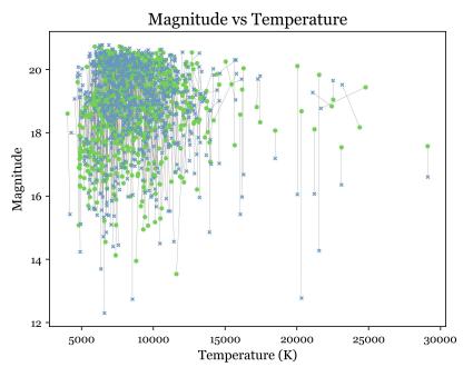
Figure 5. Apparent Magnitude-Temperature graph of the D*Z (blue) and their matched DA (green) white dwarfs using distance method (gray lines connect each DA to its matched D*Z)
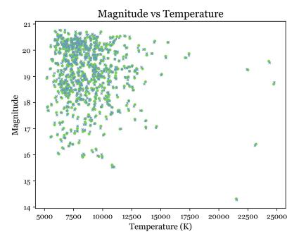
Figure 6. Apparent Magnitude-Temperature graph of the D*Z (blue) and their matched DA (green) white dwarfs using box method (gray lines connect each DA to its matched D*Z)
The concept behind the method used to get the final results was quite similar to that used in the previous one. Once again, each D*Z and DA white dwarf was plotted on an Apparent MagnitudeTemperature graph. This time, however, magnitude was kept in the logarithmic scale. Then, I selected each D*Z and drew a box with sides long on the temperature axis and units long on the magnitude axis around it, with the D*Z at its center. Finally, I picked at random a DA white dwarf that resided within this box and matched it with the D*Z. If there were no DAs inside the box, the D*Z was scrapped from the list. Any unmatched DAs were also removed.
This method worked well and produced promising magnitude and temperature distributions. As shown in Figure 6, the visualization of this new Apparent Magnitude-Temperature diagram, each metal-polluted white dwarf is significantly more alike its matched DA counterpart in both the temperature and magnitude axes.
While the matching had successfully trimmed the DA subset and created two similar samples, once I plotted the mass distribution histogram (fig. 7), an unexpected result emerged. The distribution had systematically more DAs than D*Zs for masses lower than about 0.65 M☉, which indicated that the DA sample was not an optimal representative for DA white dwarfs. This possibility risked faulty or skewed results.
Because of this setback, I used different types of white dwarfs: DCs and DZs. The process mentioned before was repeated. While the procedure was almost identical to that followed when using the DA sample, one difference was in the assignment of the correct temperature and mass variables. As mentioned above, DC white dwarfs can have either an H-dominated or He-dominated atmosphere, or one with a mix of the two elements. This made selecting the correct atmosphere parameters (mass and temperature) for these white dwarfs more complicated. However, following Gentile Fusillo’s recommendation, I assigned DCs with
effective temperatures greater than 11,000K values for atmospheres dominated by He, DCs with temperatures between 11,000K and 5,500K values for mixed atmospheres, and DCs with temperatures lower than 5,500K parameters for H-dominated atmospheres.
After the correct values were determined, the DC and DZ sublists were removed of any unwanted white dwarfs, the DC list was modified down to the length of the DZ subset (311 white dwarfs per set), and the temperature and magnitude distributions (figs. 9, 10) were plotted. Once again, the algorithm worked well, providing two nearly identical distributions in temperature and magnitude. This was further seen in the Apparent MagnitudeTemperature graph (fig. 11), which showed little difference in these parameters for matched white dwarfs.
This time, however, the mass distribution (fig. 12) of the low-mass white dwarfs was much closer to that previously
expected, and there were no signs of a systematic issue with the data, indicating that this DC sample was a good representation of DC white dwarfs.
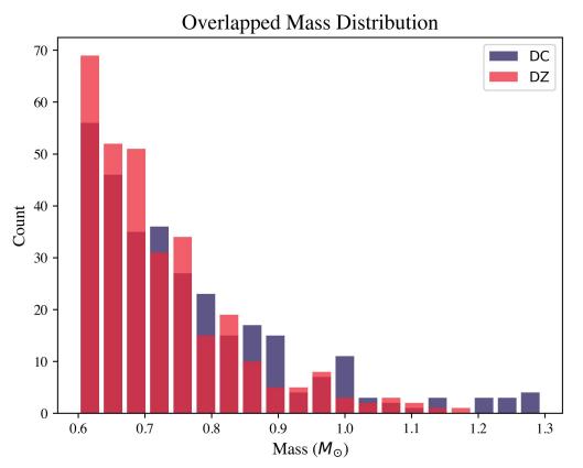
Therefore, results for this study were drawn from the comparison of the DC and DZ sublists. Thanks to a more representative sample, the presence of massive DZs could be analyzed, and results and conclusions could be drawn.
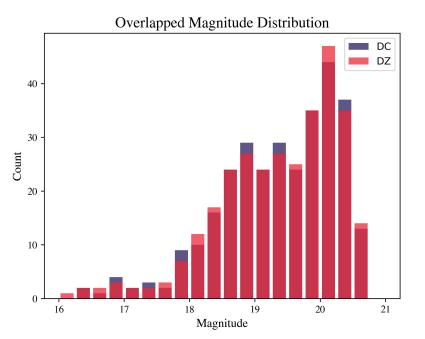
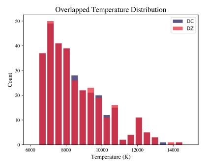
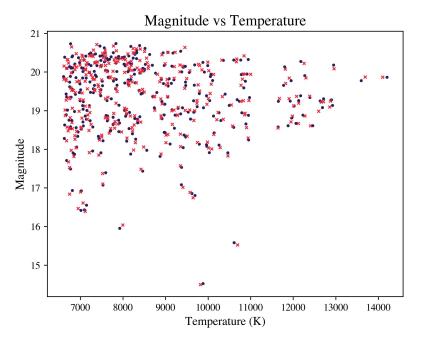
Figure 11. Magnitude-Temperature graph of the DZ (blue) and their matched DC (red) white dwarfs using box method (gray lines connect each DC to its matched DZ)
12.
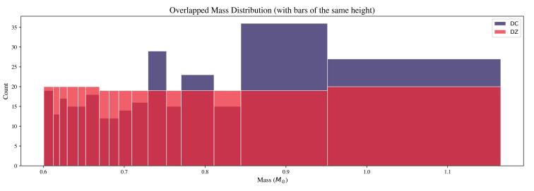
Figure 13. Overlapped Mass Distribution of DC and DZ white dwarfs with DZ bars of the same height
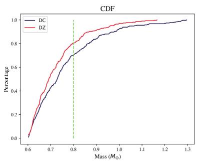
Figure 14. Overlapped Mass Cumulative Distribution Function (CDF)of DC and DZ white dwarfs
Results
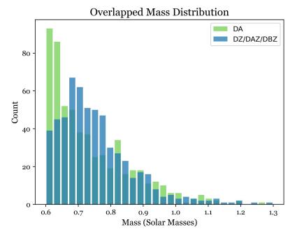
The first plot that was graphed from the data acquired to analyze the results was a regular, overlapped mass distribution histogram of the two subsets (fig. 12). This was the first step to understanding if there indeed was a lower amount of DZ white dwarfs with a mass greater than 0.8 M☉ compared to the control sample of DC white dwarfs. This graph does give an indication that fewer massive DZs are present in the sample compared to massive DCs. However, because of the relatively small total number of white dwarfs in each sample, there were very few massive DCs and DZs, so it was difficult to analyze any discrepancy using this graph.
Therefore, a similar graph, shown in Figure 13, was also plotted to better visualize the distribution at the massive end. This histogram, similar to the previous one, represented the overlapped mass distribution of the two white dwarf subsets, but this time all
the DZ bars were the same height and contained similar numbers of white dwarfs (roughly 20 white dwarfs per bar). Because of the higher presence of lower-mass white dwarfs, this resulted in more narrow histogram bars on the lower-mass end of the sample.
However, the opposite was true for the massive end. Since fewer massive white dwarfs were present in the histogram, the bars were much thicker (covered more mass) as the mass increased. While this resulted in worse resolution of the massive end, it also made it more clear that there were substantially more DCs than metal-polluted white dwarfs with mass greater than 0.8 M☉.
To further confirm what these graphs showed was was the cumulative distribution function (CDF), which plotted the cumulative percentage of white dwarfs per mass (fig. 14). The dashed line at 0.8 M☉ is there to better visualize the separation between massive and non-massive dwarfs. As displayed in the CDF and made clearer thanks to the dashed line, around 30% of
the DC list is composed of massive white dwarfs, but only around of the DZ subset is. Since the subsets have the same number of white dwarfs, these percentages indicate fewer massive DZs than DCs.
These three graphs clearly show that, just as in the UV sample, there are fewer massive metal-polluted white dwarfs. Even using white dwarfs with effective temperatures colder than 15,000K, my study still found a lack of massive metal-polluted white dwarfs, indicating that it truly may be rare for stars with masses between roughly 4 M☉ and 8 M☉ to form planets.
The next step was analyzing if this disparity was as stark as that seen in the UV sample.
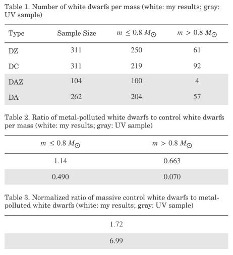
I did this by analyzing directly the data from Table 1. Here, I present the number of white dwarfs for masses ≤ 0.8 M☉ (not massive) and > 0.8 M☉ (massive) found in both my study and in the UV sample. To compare results effectively, I made Table 2.
Here, I show the ratio of metal-polluted (DZ and DAZ) white dwarfs to control (DC and DA) white dwarfs for masses ≤ 0.8 M☉ and > 0.8 M☉. Finally, to normalize the results, I divided the ratios found in Table 2 for non-massive white dwarfs with those for massive white dwarfs. This gave me Table 3. The results in this table show the ratios of control white dwarfs to metal-polluted white dwarfs for a sample with the same number of non-massive control and metal-polluted white dwarfs. Therefore, according to this data, I found a little under twice as many massive control white dwarfs as metal-polluted ones, while Ould Rouis found 7 times as many massive control white dwarfs as metal-polluted ones. Therefore, while we both found fewer metal-polluted white dwarfs with masses higher than 0.8 M☉, her results are about 4 times more drastic than mine.
Conclusion
According to this study’s result, for samples containing the same number of white dwarfs of similar apparent magnitude and effective temperature, massive DZ white dwarfs make up a smaller percentage of the full DZ sample than massive DCs do for the DC sample. This indicates that more massive white dwarfs harbor fewer planetary systems compared to less massive white dwarfs.
The overarching goal of this research was to help determine if massive main-sequence stars form fewer planets than less massive ones. Because of the lack of massive metal polluted white dwarfs, my study does support this theory. It also aligns with Ould Rouis’ findings showing fewer massive DAZs using UV observations from the HST.
Nevertheless, the findings of this research show the discrepancy between massive white dwarfs that show and do not show metals to a much milder extent than found from the UV
sample. This could indicate that the possible bias mentioned before may have, at least partly, impacted the results found by Ould Rouis.
A possible limitation of my study is the relatively small sample size. Since the experiment was carried out on distributions of only 311 DZs and 311 DCs, the results do not have impressive statistical significance. Therefore, future studies should aim to use more data to study these white dwarfs. A research encompassing both stars with surface temperatures higher than and lower than 15,000K could also provide an even more beneficial, overarching comparison.
References
Bédard, A., Bergeron, P., Brassard, P., & Fontaine, G. (2020). On the Spectral Evolution of Hot White Dwarf Stars. I. A Detailed Model Atmosphere Analysis of Hot White Dwarfs from SDSS DR12. The Astrophysical Journal, 901. https://iopscience.iop.org/article/10.3847/15384357/abafbe/meta
Dobrijevic, D., & Tillman N. T. (2022). White dwarfs: Facts about the dense stellar remnants. Space. https://www.space.com/23756-white-dwarf-stars.html
Dufour, P., Blouin, S., Coutu, S., Fortin-Archambault, M., Thibeault, C., Bergeron, P., Fontaine, G. (2016). The Montreal White Dwarf Database: a Tool for the Community. https://doi.org/10.48550/arXiv.1610.00986
Gentile Fusillo, N. P., Tremblay, P.-E., Cukanovaite E., Vorontseva, A., Lallement, R., Hollands, M., Gänsicke, B. T., Burdge,
K. B., McCleery, J., & Jordan, S. (2021). A catalogue of white dwarfs in Gaia EDR3. Monthly Notices of the Royal Astronomical Society, 508(3) , 3877-3896 .
https://doi.org/10.1093%2Fmnras%2Fstab2672
Hubblesite. (2012). Signature of a White Dwarf.
https://hubblesite.org/contents/media/images/2012/25/3052 -Image.html
Kawaler, S. D., & Dahlstrom M. (2000). White Dwarf Stars: The remnants of Sun-like stars, white dwarfs offer clues to the identity of dark matter and the age of our Galaxy. American Scientist, 88(6), 498-507.
http://www.jstor.org/stable/27858119
NASA. (n.d.). Star Basics. https://science.nasa.gov/universe/stars/ NASA. (n.d.). Types of Stars. https://universe.nasa.gov/stars/types/
Lou Baya Ould Rouis’s Oral Qualifying Exam, “Are Planets
Missing around Massive White Dwarfs?”, February 16th
2024, Department of Astronomy, Boston University
Saumon, D., Blouin, S., & Tremblay, P.-E. (2022). Current challenges in the physics of white dwarf stars. Physics Reports, 988, 1-63.
https://doi.org/10.1016/j.physrep.2022.09.001
Space & Beyond Box. (n.d.). LIFE CYCLE OF THE SUN. https://spaceandbeyondbox.com/life-cycle-of-the-
sun/#:~:text=The%20life%20cycle%20of%20the,of%20mo lecular%20gas%20and%20dust
Webb Space Telescope. (2022). Spectroscopy 101 – How Absorption and Emission Spectra Work. https://webbtelescope.org/contents/articles/spectroscopy101 how-absorption-and-emission-spectra-work