David Sadka Senior Thesis 2024 by Boston University Academy

1 Introduction

Music sentiment is the quantification of music’s mood. Prior literature in behavioral finance has attempted to use music sentiment as a proxy for investor sentiment to investigate various financial economic indicators. Edmans, Fernandez-Perez, Garel, and Indriawan (2021) show that music sentiment displays a contemporaneous relation with weekly stock market returns and predicts next-week returns. Sabouni (2018) finds that music sentiment predicts consumer sentiment and Kaivanto and Zhang (2019) document a relation to stock trading volume and future returns.

This paper presents three novel results: (a) music sentiment has a differential impact across the consumption sentiment (how optimistic consumers feel about their finances and the state of the economy) of age and income groups; (b) the impact of music sentiment displays significant time trends; and (c) music sentiment is priced in the cross-section of expected stock returns, with meaningful correlation with the momentum factor. Overall, this study highlights how music sentiment can be used to better understand various financial economic indicators.

Specifically, the top songs from the weekly Billboard Hot 100 list over the period 1962-2021 are retrieved using Pythonbased web-scraping techniques. Making use of ChatGPT, a lyric analysis of these songs is implemented to construct a monthly time-variant measure. Inspired by the analysis in Sabouni (2018), regression analysis is used to test the impact of music sentiment on both consumer sentiment (proxied by Michigan’s Consumer Sentiment Index) and market returns (proxied by the S&P 500 index). The results show that an increase in happiness in a given month significantly predicts a decrease in consumer sentiment the following month, while the contemporaneous relation between music sentiment and consumer sentiment is positive, which is

consistent with the predictions and results in Edmans, FernandezPerez, Garel, and Indriawan (2021). The results are robust to controlling for lag market returns and investor sentiment. The results suggest that individuals over-project their mood onto their consumption sentiment, which is corrected the following month.

The approach taken in this paper to research the relationship between music sentiment and economics is similar to previous papers, insofar as popular music is used to proxy investors’ mood. Yet, the constructed measure only uses textual analysis of lyrics. Despite the pitfalls of simple NLP to analyze music lyrics, this strategy allows the paper to extend the time period to the past 60 years and provide more robust results and further novel insight. Also, one potential concern with using music to proxy mood is that individuals may listen to music to combat their moods (one may listen to happy music to combat sadness, for example), instead of listening to music that reflects their mood. However, prior research has shown that individuals’ music preferences correspond to their emotional state (North and Hargreaves (1996)). In addition, Saarikallio and Erkkil¨a (2007) show that sad individuals choose to listen to sadder music to vent their emotions or achieve closure.

This paper demonstrates that extending the sample period of the music sentiment allows for an investi- gation of this nonstable time trend. Indeed, the happiness and consumer sentiment relation strengthens over time. The increase in accessibility of music in mobile devices and vehicles (especially in the 21st century) may be contributing to this effect. Further partitioning consumer sentiment by age and income, the results show that the documented time trend is more apparent among the younger age group and the upper-income group. This may be explained by the fact that younger people listen to more music and are thus more affected by it, and that higher-income individuals may have more

time to listen to music, which in turn is reflected in their consumption habits.

Finally, the paper studies the cross-sectional asset prices of sentiment-sensitive stocks. Happiness significantly prices the cross-sectional expected stock returns. That is, high-musicsensitive stocks, those that rise in value during months of happy music sentiment and drop in value during unhappy-musicsentiment months, outperform low-music-sensitive stocks by an average of roughly 2.2% per annum (t-statistic of 2.1). This can be interpreted as compensation for the risk of investing in sentimentsensitive stocks. A Fama-French factor analysis shows that this happy risk premia is primarily captured by the momentum factor. This result implies that the risk in holding stocks that are happysensitive (related to individuals’ emotions) is related to the performance of the momentum strategy, suggesting that individuals continue buying recently outperforming stocks when they feel happy.

2 Data

2.1 Construction of Sentiment Measure

The weekly Billboard Hot 100 list from 1962 up to the end of 2021 is retrieved to construct a weekly measure of music sentiment.1 For each song that appears on a list during this time span, its lyrics are downloaded by searching the song name and artist on lyricfinder.org.2 A word-based lyric analysis is performed by obtaining a set of 200 keywords from ChatGPT for the happy

1 Billboard (2023). The Hot 100 Chart. Billboard. https://www.billboard.com/charts/Hot 100/ 2 Lyricfinder.org. Retrieved October 10, 2023, from https://www.lyricfinder.org

emotion.3 The happy sentiment of a song is defined to be (after the removal of stopwords) the percentage of the song’s lyrics that appear in the set of happy keywords. The sentiment of song s is denoted Happy ss.

Over the 60-year sample, 27,689 unique songs appear on the Billboard Hot 100 list. On average, the highest rank that a given song reaches in this sample is 46.6, and around 49% of songs rank in the top 40 at least once. Furthermore, the average Happy s of songs that reach the top 40 is 2.89% whereas the average Happy s across all songs is 2.81%. Note that due to online lyric availability, only 25,788 songs have a Happy s score. The histogram of Happy s is plotted in Figure 1.

For reference, the Beatles have 15 songs that appear on the Hot 100 with a Happy s above 7%, Adele has 13 such songs with a Happy s less than 2%, and Billie Eilish has 18 songs with a Happy s less than 2%.

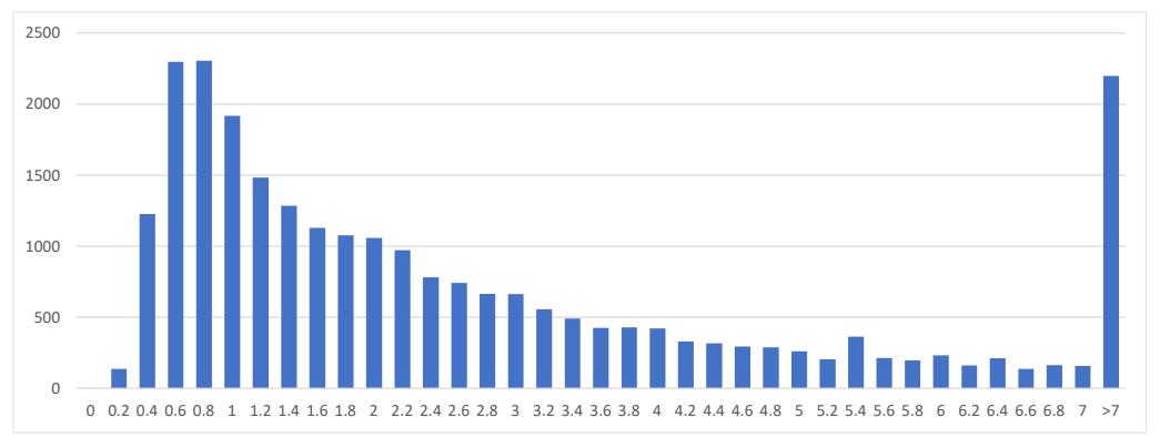
Figure 1: The distribution of the song-level sentiment measure Happy s

3 3OpenAI. (2022, November 30). ChatGPT. Chat.openai.com. https://chat.openai.com

2.2 Time Series

Define the rank function rank(w, i) that outputs the song s that is ranked i on the Hot 100 list for week w. The happy sentiment of week w is then given by the following rank-based weighted average:

where n is the number of top songs. For example, when calculating Happy ww,100, the 1st ranked song in week w receives a weight of 100 and the 100th ranked song receives a weight of 1. Then, a monthly measure of sentiment Happy m is given by averaging Happy w over the weeks that span each month. Note that the Hot 100 list is released every Saturday for the previous week, and the weeks included in the calculation of Happy mm are the weeks whose Saturdays are in month m. Thus, the week that ends on Saturday August 1, 2020 for example counts towards Happy m of August 2020 and not July 2020. This way of calculation is not subject to look-ahead bias.

Despite using a weighted average to appropriately weigh the effect of lower ranked songs on the sentiment measure, these lower-ranked, volatile songs on the list may influence the accuracy of the measure and generate noise in the data. Thus, as is the standard in the music industry, this paper will focus on the sentiment measure of the top 40 songs. For the remainder of the paper, Happy w and Happy m will refer to the sentiment measures that use the top 40 songs.

To validate the Happy measure of sentiment, the overall Happy m time series as well as the time series over a few particular time spans are plotted.

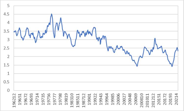
Figure 2: The time series of Happy m over the sample period, January 1, 1962 through December 31, 2021

Figure 2 displays the general trend of a decrease of the Happy m over the last 60 years, which is consistent with the trend of increasing suicide rates over the last two decades (correlation between changes in annual suicide rates and changes in annual Happy sentiment is -20%).4

4 Data retrieved from the CDC website: https://www.cdc.gov/nchs/products/databriefs/db464.htm.

The happy sentiment measure is also consistent with expected sentiment shocks around various significant social and economic events over the last 60 years. As shown in Figure 3, the Happy m takes a dramatic decrease at the time of the oil and inflation crises at the end of the 1970s, which is expected with economic frustration and the end of the Vietnam War, and rises afterwards. In Figure 4, Happy m decreases leading up to the financial crisis of 2008, but rebounds in the following months. A similar behavior is seen more recently in reaction to the global pandemic in 2020.

Another music sentiment measure that is used in the literature (Sabouni (2018) and Edmans, Fernandez- Perez, Garel, and Indriawan (2021)) is Spotify’s valence metric, which measures the happiness of a song based on the likelihood one will feel happier after listening to the song. A regression test of valence on Happy s shows a significant relationship between these two measures (t-statistic of 5.65). The happy measure is more suitable for this paper however due to many songs not being readily available on Spotify, especially older ones. Most of the prior work has been conducted using data from the past two decades whereas this paper extends the sample period to 60 years by scraping the lyrics of these songs online.

2.3 Music Tone Dynamics

The existence of songs and their popularity can be viewed as an equilibrium outcome of supply and demand for music. The consumers’ demand is reflected in the sentiment of the top songs as well as the sentiment of the songs that climb the rankings because the rankings are controlled by the consumers.

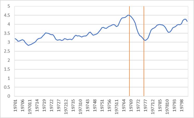
Figure 3: The time series of Happy m from January 1970 through December 1979

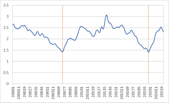
Figure 4: The time series of Happy m level from January 2000 through December 2021

For example, if consumers are in the mood for happy music one week, then one might expect happy songs to climb the Hot 100 rankings more than average this week. Therefore, an analysis is performed to explore both if happier songs climb the Billboard Hot 100 rankings quicker than sad songs, and how the overall sentiment of the top songs impacts the time it takes to climb the rankings. In other words, does the presence of happier songs in the top 40 make it so that it is quicker for happier songs outside the top 40 to enter the top 40?

A dummy variable is used to classify happy and unhappy songs. This variable assigns a value of 1 for songs with a Happy s in the top 10 percentile and 0 for songs with a Happy s in the bottom 10 percentile, with the rest of the songs excluded from this analysis. Separately, the continuous Happy s itself is also used for all songs. For each song s that attains a top 40 ranking at some point in the sample period, the number of weeks taken to reach this ranking from the first time it appears on the Hot 100 list is calculated (denoted by the variable Rises). The distribution of the Rise variable is plotted in Figure 5. The mode is 3 weeks, with a long tail after 20 weeks (1.3% of the distribution is above 20 weeks). Given the 20+ week outliers, they are omitted from the analysis in Table 1. Without these songs, the distribution has a median of 3 weeks with a standard deviation of 3 weeks. In addition, for each song s, the average of Happy w between the weeks that the song first entered the top 100 and the top 40 is computed and denoted Happy rises.

The results in Table 1 first suggest that happy songs (those in the top 10%) make it to the top 40 almost 2 weeks faster on average than un-happy songs (those in the bottom 10%). Furthermore, the significant negative Happy rises coefficient suggests that the happier the top 40 songs are, the quicker it takes songs (in general) to enter the top 40. Finally, the significant positive coefficients of the pairwise multiplication of Happy rises

and 10% Dummy or the continuous Happy s indicates that when the top 40 songs exhibit happiness, it takes longer for happier songs to enter the top 40, implying that perhaps there is a limit to how many happy songs people will listen to at once.

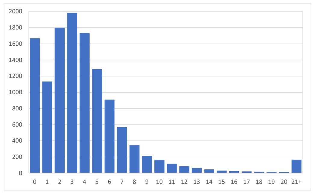
Figure 5: The histogram of the variable Rise: the number of weeks it takes a song to reach the top 40 from when it first

appeared on the Hot 100 list. Songs that never attain a top 40 ranking are not included.

2.4 Seasonality of Sentiment

As is the case with other mood-influenced measures, such as consumer and investor sentiment, it is reasonable to test for seasonality in the data due to the seasonality of an individual’s mood. For example, particularly during happy times like Christmas and the beginning of summer, individuals’ mood is expected to be happier than in the winter. Both consumer and investor sentiment are seasonal and the data is pre-adjusted accordingly in their construction. To test for seasonality in Happy m, monthly averages are first examined.

The clear pattern is the increased happy levels in the winter months of November, December and January. A Kruskal-Wallis test, which tests whether samples originate from the same distribution, is performed by separating the data into two groups: data from November, December, and January in one group, and the other months in another group. The data is then ranked across all groups together, from 1 to N, where N is the total number of observations. If there are ties, the common rank assigned to these data points is the average of their ranks had they not been tied. The test-statistic, H, is calculated via the following equation:

where g is the number of groups (2 in this case), ni is the number of observations in group i, rij is the rank among all observations of the jth observation of group i, ri is the average rank of all observations in group i, and r = ½ * (N + 1) is the average rank among all observations. The null hypothesis that the medians of the groups are the same is rejected if the H statistic is greater

than the critical value Hc, which is estimated by the critical χ2 value with g − 1 degrees of freedom.

The result of the Kruskal-Wallis test (P-value = 0.0182) suggests that the happy measure in winter holiday months is significantly different than in the rest of the year, indicating a need for seasonal adjustment. An explanation for these differences is the popularity of Christmas songs (which tend to be happier) in these holiday times. Songs such as Mariah Carey’s “All I Want for Christmas is You” rise towards the top of the list frequently during these months and contribute to the seasonal happy trend seen in Figure 6.

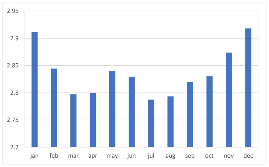
Figure 6: The monthly average Happy m over the sample period, January 1, 1962 through December 31, 2021

To correct for this seasonality, the measure is adjusted by subtracting the previous year’s Happy m that month from the current month’s Happy m:

Happy madj,t = Happy mt − Happy mt−12. (3)

This seasonally adjusted measure is used in the analyses in the remainder of the paper.

2.5 Validation of Measure

To further validate the happy measure of sentiment, regressions with Happy m as the dependent variable are performed to test whether economic indicators such as consumer sentiment, investor sentiment, and market returns, explain the variability in Happy m. The results displayed in Table 2 show that none of these indices explain Happy m contemporaneously, nor do they show any significant predictive ability. This emphasizes the exogeneity (with respect to the other economic variables) of the happy sentiment measure.

2.6 Other Variables

Analyses are performed with various financial economic indicators. Weekly and monthly stock market returns dating back to 1962 are obtained from the Ken French data library.5 Baker and Wurgler (2006)’s investor sentiment data (1965-2021) are used to proxy investor sentiment. Michigan’s Surveys of Consumers Index data, which begins in 1978, are used to proxy consumer sentiment.

5 Ken French Data Library https://mba.tuck.dartmouth.edu/pages/faculty/ken.french/data library.html

This sentiment index also partitions the data into different segments based on various criteria such as age, income, and region. It also provides data on consumers’ sentiment towards their personal finances, business conditions in the next 12 months, buying conditions, and others.6 This paper mainly uses the age and income-level data to investigate the relationship of music sentiment and these characteristics. There are three age groups (1834, 35-54 years old, and 55+ years old) and three income groups (lower, middle, and upper). Note that the sentiment indices are also appropriately seasonally adjusted.

The analyses seek primarily to explain different types of consumer sentiment in terms of music sentiment while using market returns and investor sentiment as controls in the hypothesis testing. Additional analyses are performed to investigate the crosssectional returns of stocks. These tests utilize the six Fama-French factors, the market factor (MKT-RF), size (SMB), value (HML), profitability (RMW), investment (CMA), and momentum (UMD), which are downloaded from Ken French’s website.

3 Results

3.1 General Consumer Sentiment

This paper’s main analysis concerns the relationship between music sentiment and consumer sentiment. Regression analysis is used to investigate both the contemporaneous and lag relations over the entire sample period. Table 3 shows a significantly negative relation between changes in consumer sentiment and the one- month lag of Happy m at the 1% significance level, even when controlling for the one-month lags of

6 Michigan Surveys of Consumers: https://data.sca.isr.umich.edu/data-archive/mine.php

investor sentiment and market returns. Furthermore, the contemporaneous relation is positive when controlling for the onemonth, two-month, and three-month lags of Happy m. When music happiness increases in a given month, the consumer sentiment displays a similar behavior, but the following month, the trend is reversed, suggesting a correction in the initial sentiment shock. This sentiment reversal is consistent with results from Sabouni (2018).

The contemporaneous and lagged relation between consumer sentiment and music sentiment is further analyzed over time. This is done via a regression model, estimated every 5 years using a 20-year rolling window as follows:

(Consumer Sentiment)t =α + β1 ∗ Happy mt + β2 ∗ Happy mt−1 + Controlst + Controlst−1 + ϵt. (4)

That is, the first regression consists of the 239 monthly observations from January 1978 through December 1997 (the consumer sentiment data begins in January 1978, meaning the first observation for changes in consumer sentiment is February 1978), the second regression consists of the 240 monthly observations from January 1983 through December 2002, etc. Once again, market returns and changes in investor sentiment are used as controls.

The results in Table 4 show that the positive contemporaneous relation between consumer sentiment and Happy m, and the corresponding negative lagged relation increase in both significance and strength over time. From 1978 to 1997, every 1% increase in Happy m in a given month corresponds to a 0.081 point increase in the consumer sentiment that month and a 0.438 point decrease the following month. However, in the final 19 years of the sample period, the same increase in Happy m corresponds to a 1.591 point increase in consumer sentiment the same month and a

2.405 point decrease the following month (t-statistics of 1.92 and2.92 respectively). For reference, the distribution of the change in consumer sentiment scores in the sample period demonstrates a standard deviation of 4 points, with a 25th percentile of -2.3 and a 75th percentile of 2.5. The distribution of the monthly change in Happy m from 1978 to 2021 exhibits a standard deviation of 0.36% with a 25th percentile of -0.21% and a 75th percentile of 0.23%. Economically, this means that recently, a 1 standard deviation increase in monthly happy sentiment has been associated with a 0.14 standard deviation increase in consumer sentiment and a 0.22 standard deviation decrease the next month, where 14.3% of this variation is explained by the changes in Happy sentiment. This suggests that music sentiment has affected consumers more in recent times, which can be attributed to the increased availability of music through online outlets and the reduced price of CDs in the 21st century.

3.2 Age-Level Consumer Sentiment

To investigate the impact of age on the consumer-music relationship over time, a very similar regression model (estimated every 5 years using a 20-year rolling window) as the one used for general consumer sentiment is used with market returns and changes in investor sentiment as controls for the three different age groups i ∈ {18-34, 35-54, 55+}. The following model is used:

Tables 5, 6, and 7 all display the same trend over time as the general consumer sentiment, with the strength and significance of the positive contemporaneous relation and the negative lagged relation increasing over time. Yet, as Figures 7 and 8 highlight, the strength and significance of the relationship at the beginning of the

sample period is noticeably different for the age groups, where it is less pronounced for the younger age group. However, over time, the strength of the relation for the younger age group has increased the most, and all three age groups converge to similar strength and significance in both the contemporaneous and lagged relations towards the end of the sample period. From 1997 to 2021, the coefficient of Happy mt increases by 2.613 (t-statistic increases from -0.72 to 1.63), implying that every 1% increase in Happy m in a given month has resulted in a 2.613 greater increase in consumer sentiment points that month in 2021 than in 1997. Likewise, the coefficient of Happy mt−1 decreases by 3.076 (tstatistic decreases from 0.58 to -2.03). Thus, a 1% increase in Happy m in a given month has resulted in a 3.076 greater decrease in consumer sentiment points the following month from the beginning to the end of the sample period. The notion that music sentiment has a greater impact on the younger age group may be a result of younger adults listening to music more than older age groups.

3.3 Income-Level Consumer Sentiment

The impact of income on the consumer-music relationship over time is tested using again a very similar regression model (estimated every 5 years using a 20-year rolling window) as the one used for general consumer sentiment, with market returns and changes in investor sentiment as controls for the three different income groups i ∈ {Lower, Middle, Upper}. The following model is used:

Tables 8, 9, and 10 all generally display the same trend over time as the general consumer sentiment and age groups, with

the strength and significance of the positive contemporaneous relation and the negative lagged relation increasing over time. However, as Figures 9 and 10 display, the strength and significance of the relation among all three groups is similar at the beginning of the sample period, unlike the relations of the age groups. These relations then diverge over time, with the upper income group exhibiting the strongest relation of the three groups. Combining this with the result found for the younger age group, this may suggest that music sentiment predominantly affects the high young income earners’ sentiment towards consumption.

3.4 Cross-Sectional Stock Pricing

Since Happy m seems to demonstrate a significant and dynamic relationship with consumer sentiment, it is reasonable to investigate whether the happy sentiment measure leads to changes in expected cash flow, in turn affecting expected stock returns. A Fama-Macbeth regression is used to estimate the risk premia for trading Happy-sensitive stocks. In other words, do stocks that rise in times with a high happy music sentiment, and do the opposite in times of low happy sentiment, subsequently outperform on average? If so, this can be interpreted as a return premia to compensate investors holding Happy-sentiment risk.

The Fama–MacBeth regression is a method that estimates the risk premia for any risk factors that are expected to determine asset prices. This estimation is done in two steps. First, a monthly time-series regression of the risk factor (Happy m in this case) on each of the n stocks’ returns that have appeared in the S&P 500 since 1962, controlling for overall market returns, is performed as follows:

Rn,t = αn + βnHappy mt + β′ Mktt + ϵn,t

For each stock, a yearly Happy and Market beta are estimated by running a 3-year (36-month) regression from the equation above. Then, cross-sectionally, for each year, regress the stock’s end of year returns against the yearly beta coefficients calculated in the previous step. Note that before running this regression, the Happy m beta coefficients of a given year are standardized by dividing each coefficient by the standard deviation of all the Happy m beta coefficients that year. The same is done for the Market betas. The yearly beta coefficients are denoted with aˆ.

Ri,1 = γ1,0 + γ1,1βˆ i + γ1,2βˆ′ + ϵi,1 (7) Ri,2 = γ2,0 + γ2,1βˆ i + γ2,2β

′ + ϵi,2

Ri,T = γT,0 + γT,1βˆ i + γT,2β

′ + ϵi,T

In this case, T represents the number of years in the sample period, and Ri,Y represents the ith stock’s return at the end of Y th year. A hypothesis test is then conducted on the mean of γ1,1, ..., γT,1 – the estimated coefficients of the Happy betas – to determine the desired risk premia.

The Fama-Macbeth regression for Happy m results in a statistically significant risk premia of 2.18% per year (t-statistic of 2.01). That is, Happy m-sensitive stocks earn, on average, 2.18% per year more than non-Happy m-sensitive stocks.

3.5 Fama-French Factor Analysis Results

The final result looks at the 6-factor Fama-French model to see if the risk of trading Happy-sensitive stocks is captured in the

six Fama-French factors: Market risk (Market returns), size (SMB -Small Minus Big), value (HML - High Minus Low), profitability (RMW - Robust Minus Weak), investment (CMA - Conservative Minus Agressive), momentum (UMD - Up Minus Down). These factors provide a more comprehensive framework for understanding the complexities of stock returns and help investors make more informed decisions by considering multiple dimensions beyond just market risk.

To test if the happy risk premium is captured by the factors, a series of regressions are performed with the monthly time-series of the γ coefficients of the Happy m betas in Equation (7) and the factors (see Table 11 for the results). When the Happy m gammas are regressed on each of the Fama-French factors separately, the regression intercepts (interpreted as risk-adjusted returns) remain insignificant, except in the case of the momentum factor. The momentum factor coefficient is highly significant (t-statistic of 7.07), and the regression intercept drops to 1.14% annually (a drop of roughly half the magnitude). Similar results are obtained when all factors are used simultaneously (multi-variate regression). The relation of the Happy m return series to momentum suggests that individuals continue buying recently outperforming stocks (i.e., momentum) in times with happier popular music.

4 Discussion

The keyword approach for the NLP analysis in this paper works well, but to improve the sentiment measure, other factors could be taken into consideration. For example, since this paper extends the data’s time period and uses music dating back to the 1960s, it is reasonable to investigate how emotion may be conveyed differently in different eras of music. Thus, the basket of happy words obtained for the entire sample period for the measure could be altered every decade to account for the change in

language over time. Furthermore, each genre of music may convey emotion differently through their lyrics. The prominence of jazz and swing in the 60s and 70s, rock in the 80s and 90s, and pop in the 2000s, may call for an adjustment to the music sentiment measure based on the way each genre uses words.

Other music sentiment papers investigate not only happiness or positivity, but a plethora of other emotions as well, such as sadness, anger, fear, and surprise, which are all worth a deeper look. For instance, the sad measure of sentiment may not only be capturing the absence or opposite of happiness, but another nuance of the lyrics as well, which may provide additional insights into the results discussed in this paper. Analyses involving these other emotions are left to future research.

5 Conclusion

This paper re-examines prior literature that uses music sentiment to explain economic variables while extending the sample period to the 1960s, and separating consumers by age and income groups. The analyses reveal significant time trends, perhaps due to technological trends in access to music, as well as significant variation across consumer types. The paper demonstrates how one can measure individuals’ feelings and tangibly show they can have an aggregate effect on economic variables.

References

Baker, M, and J Wurgler (2006). Investor Sentiment and the CrossSection of Stock Returns. Journal of Finance 61(4). Pp 1645-1689.

Edmans, A., Fern´andez-P´erez, A., Garel, A., & Indriawan, I. (2022). Music sentiment and stock returns around the world. Journal of Financial Economics 145(2A), pp 234254.

Fama, E.F, and K.R. French (2018). Choosing factors. Journal of Financial Economics 128(2), pp 234- 252.

Fama, E.F, and J.D. MacBeth (1973). Risk, Return, and Equilibrium: Empirical Tests. Journal of Political Economy 81(3), pp 607-636.

North, A.C., Hargreaves, D.J., 1996. Situational influences on reported musical preference. Psychomu- sicol. J. Res. Music Cognit. 15, 30–4.

Kaivanto, K., & Zhang, P. (2019). Popular music, sentiment, and noise trading. Economics Working Paper Series, Lancaster University.

Saarikallio, S., Erkkil¨a, J., 2007. The role of music in adolescents’ mood regulation. Psychol. Music 35, 88–109.

Sabouni, H., 2018. The rhythm of markets. Claremont Graduate University. Unpublished working paper.

Table 1: Music Tone Dynamics. The dependent variable is the number of weeks between a song’s first appearance on the Hot 100 list and its first appearance in the top 40 (Rises). Songs that took more than 20 weeks to do so are omitted from these regressions. The variable Happy rises denotes the average of the aggregate Happy w measure over these weeks, (10% Dummy)s denotes the discrete dummy variable that assigns 1 and 0 to the top 10% and bottom 10% of happy songs respectively, disregarding the middle 80%, and Happy ss is the Happy s of each song (includes all songs). This regression is run at the song-level. The tstatistics are reported in brackets.

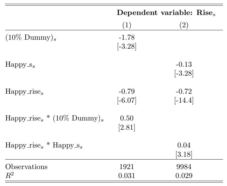
Table 2: Validation of the happy sentiment measure. This table reports regression results from January, 1962 through December, 2021. The dependent variable is the adjusted Happy m. The other variables are changes consumer sentiment (Consumert), changes in one-month-lagged consumer sentiment (Consumert−1), changes in investor sentiment (Investort), changes in one-monthlagged investor sentiment (Investort−1), market returns (Mktt), and one-month-lagged market returns (Mktt−1). Standard errors are reported in parentheses.

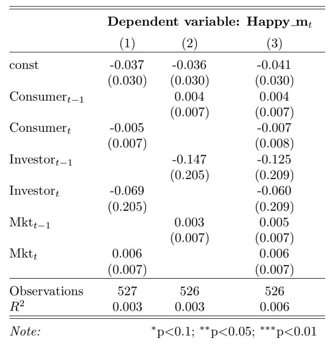
Table 3: Consumer Sentiment and Happy. This table reports regression results from January, 1962 through December, 2021. The dependent variable is the monthly change in overall consumer sentiment. The variable Happy mt denotes the contemporaneous adjusted happy measure and Happy mt−n denotes the n-monthlagged adjusted monthly happy measure. The control variables are changes in investor sentiment (Investort), changes in one-month-lagged investor sentiment (Investort−1), market returns (Mktt), and one-month-lagged market returns (Mktt−1). Standard errors are reported in parentheses.

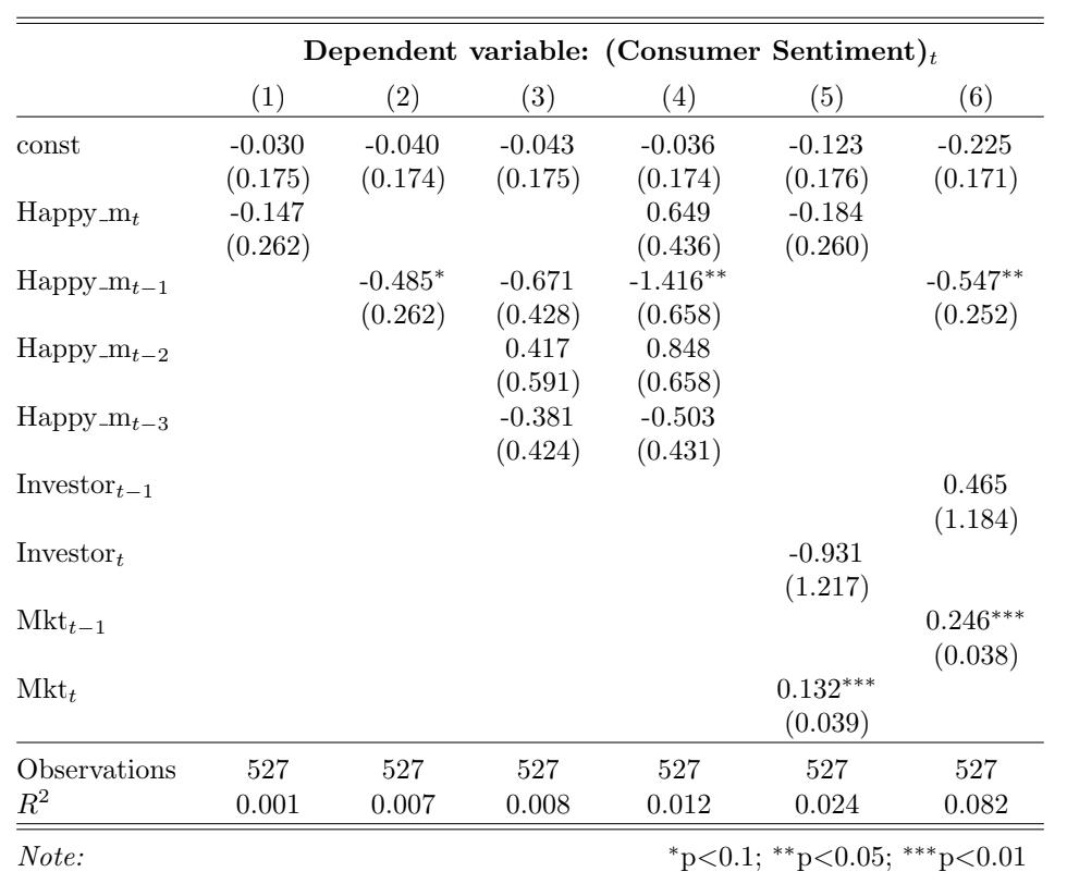
Table 4: Consumer Sentiment and Happy m Over Time. This table reports the regression estimates from Equation (4) for the contemporaneous and lagged Happy m variables. Each column reports the regression results using the 20-year time window that ends in December of the labeled year. The dependent variable is the monthly change in overall consumer sentiment. The variable Happy mt denotes the contemporaneous adjusted happy measure and Happy mt−1 denotes the one-month-lagged adjusted happy measure. The control variables (estimates not reported in this table) are changes in investor sentiment, changes in one- month-lagged investor sentiment, market returns, and one-month-lagged market returns. The t-statistics are reported in brackets.

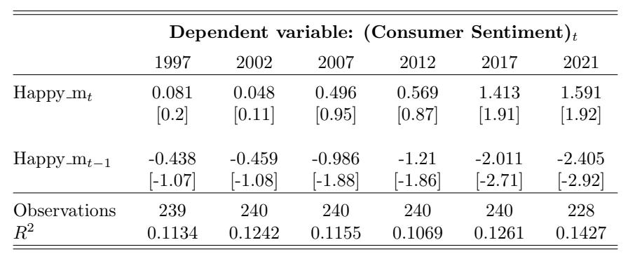
Table 5: Consumer Sentiment for Ages 18-34 and Happy m Over Time. This table reports the regression estimates from Equation (5) for the contemporaneous and lagged Happy m variables with i = 18-34 years old. Each column reports the regression results using the 20-year time window that ends in December of the labeled year. The dependent variable is the monthly change in overall consumer sentiment. The variable Happy mt denotes the contemporaneous adjusted happy measure and Happy mt−1 denotes the one-monthlagged adjusted happy measure. The control variables (estimates not reported in this table) are changes in investor sentiment, changes in one-month-lagged investor sentiment, market returns, and one-month-lagged market returns. The t-statistics are reported in brackets.

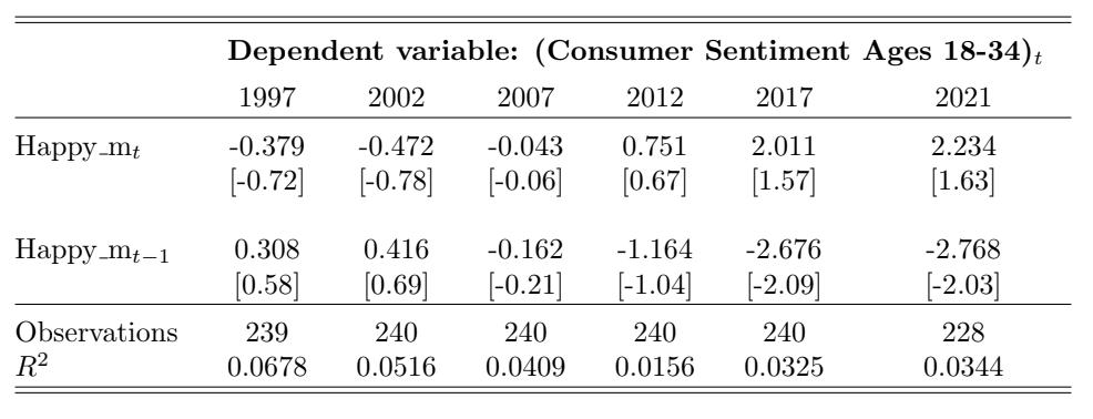
Table 6: Consumer Sentiment for Ages 35-54 and Happy m Over Time. This table reports the regression estimates from Equation (5) for the contemporaneous and lagged Happy variables with i = 35-54 years old. Each column reports the regression results using the 20-year time window that ends in December of the labeled year. The dependent variable is the monthly change in overall consumer sentiment. The variable Happy mt denotes the contemporaneous adjusted Happy measure and Happy mt−1 denotes the one-monthlagged adjusted Happy measure. The control variables (estimates not reported in this table) are changes in investor sentiment, changes in one-month-lagged investor sentiment, market returns, and one-month-lagged market returns. The t-statistics are reported in brackets.

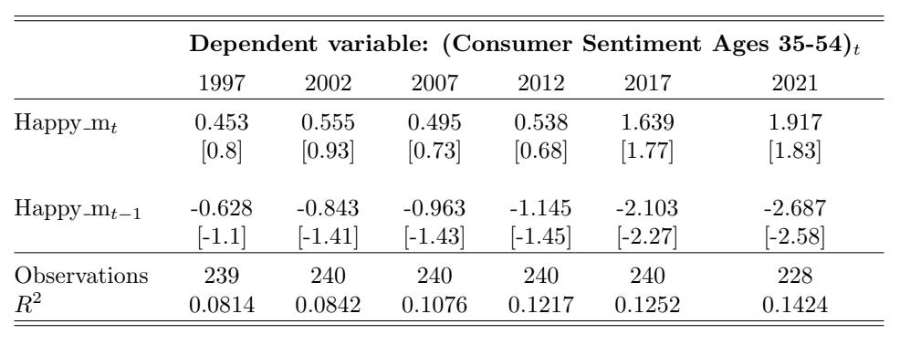
Table 7: Consumer Sentiment for Ages 55+ and Happy m Over Time. This table reports the regression estimates from Equation (5) for the contemporaneous and lagged Happy m variables with i = 55+ years old. Each column reports the regression results using the 20-year time window that ends in December of the labeled year. The dependent variable is the monthly change in overall consumer sentiment. The variable Happy mt denotes the contemporaneous adjusted happy measure and Happy mt−1 denotes the one-monthlagged adjusted happy measure. The control variables (estimates not reported in this table) are changes in investor sentiment, changes in one-month-lagged investor sentiment, market returns, and one-month-lagged market returns. The t-statistics are reported in brackets.

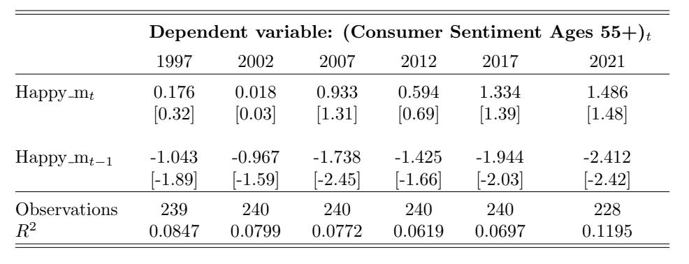
Table 8: Consumer Sentiment for the Lower Income Group and Happy m Over Time. This table reports the regression estimates from Equation (6) for the contemporaneous and lagged Happy m variables with i = Lower. Each column reports the regression results using the 20-year time window that ends in December of the labeled year. The dependent variable is the monthly change in overall consumer sentiment. The variable Happy mt denotes the contemporaneous adjusted happy measure and Happy mt−1 denotes the one-monthlagged adjusted happy measure. The control variables (estimates not reported in this table) are changes in investor sentiment, changes in one-month-lagged investor sentiment, market returns, and one-month-lagged market returns. The t-statistics are reported in brackets.

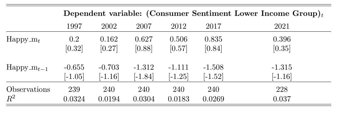
Table 9: Consumer Sentiment for the Middle Income Group and Happy m Over Time. This table reports the regression estimates from Equation (6) for the contemporaneous and lagged Happy m variables with i = Middle. Each column reports the regression results using the 20-year time window that ends in December of the labeled year. The dependent variable is the monthly change in overall consumer sentiment. The variable Happy mt denotes the contemporaneous adjusted happy measure and Happy mt−1 denotes the one-monthlagged adjusted yappy measure. The control variables (estimates not reported in this table) are changes in investor sentiment, changes in one-month-lagged investor sentiment, market returns, and one-month-lagged market returns. The t-statistics are reported in brackets.

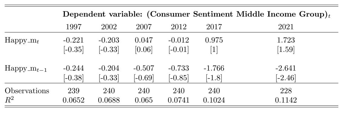
Table 10: Consumer Sentiment for the Upper Income Group and Happy m Over Time. This table reports the regression estimates from Equation (6) for the contemporaneous and lagged Happy m variables with i = Upper. Each column reports the regression results using the 20-year time window that ends in December of the labeled year. The dependent variable is the monthly change in overall consumer sentiment. The variable Happy mt denotes the contemporaneous adjusted happy measure and Happy mt−1 denotes the one-monthlagged adjusted happy measure. The control variables (estimates not reported in this table) are changes in investor sentiment, changes in one-month-lagged investor sentiment, market returns, and one-month-lagged market returns. The t-statistics are reported in brackets.

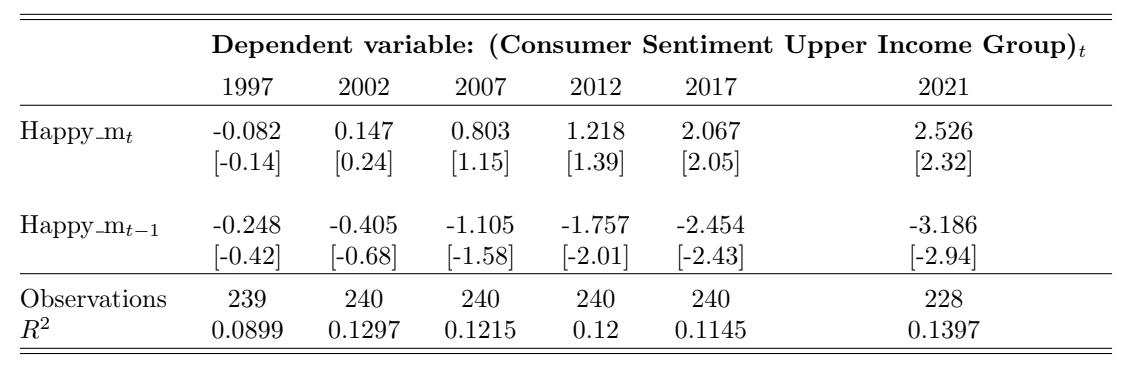
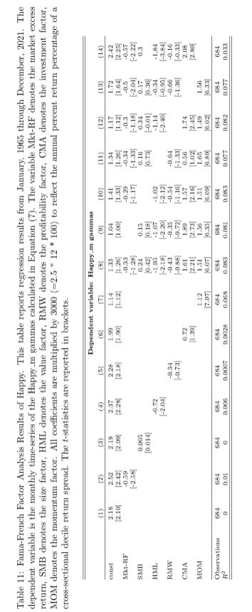
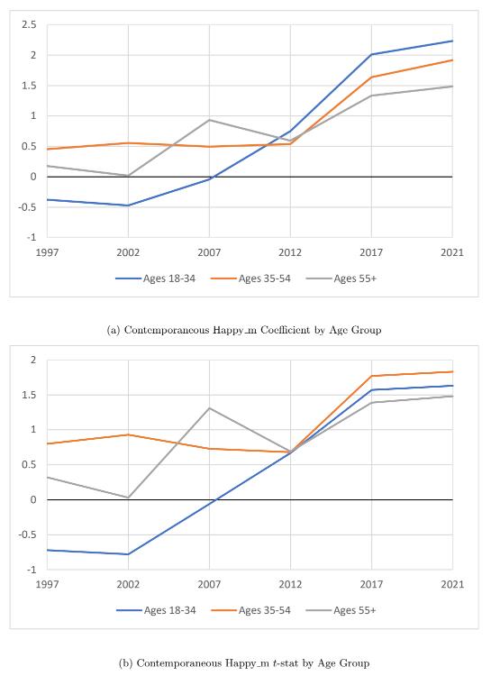
Figure 7: Contemporaneous Happy m by Age Group. This figure plots the estimated contemporaneous Happy m coefficients and t-statistics from Equation (5) for each age group, where the regressions are run using a 20-year time window that ends in December of the labeled years. The plot corresponds to the values displayed in Tables 5, 6, and 7.

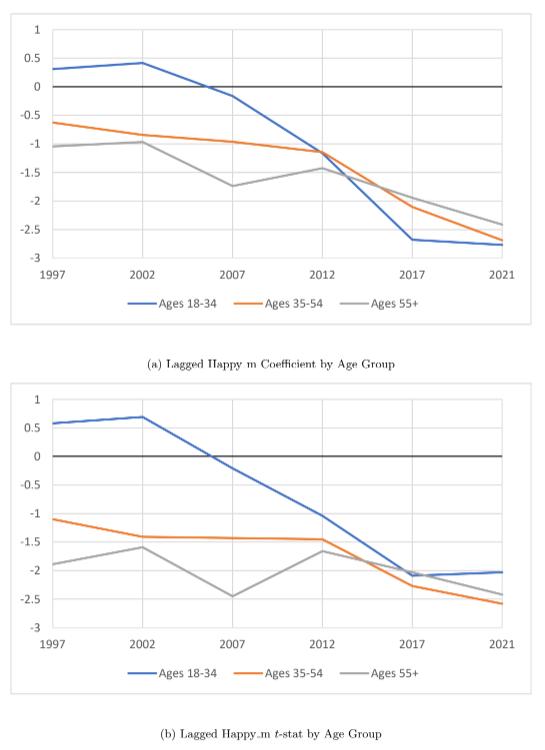
Figure 8: Lagged Happy m by Age Group. This figure plots the estimated lagged Happy m coefficients and t-statistics from Equation (5) for each age group, where the regressions are run using a 20-year time window that ends in December of the labeled years. The plot corresponds to the values displayed in Tables 5, 6, and 7.

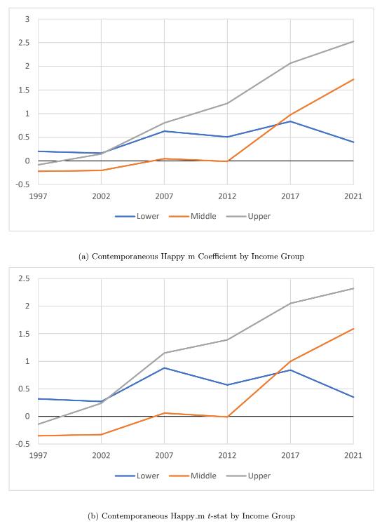
Figure 9: Contemporaneous Happy m by Income Group. This figure plots the estimated contemporaneous Happy m coefficients and t-statistics from Equation (6) for each income group, where the regressions are run using a 20-year time window that ends in December of the labeled years. The plot corresponds to the values displayed in Tables 8, 9, and 10.

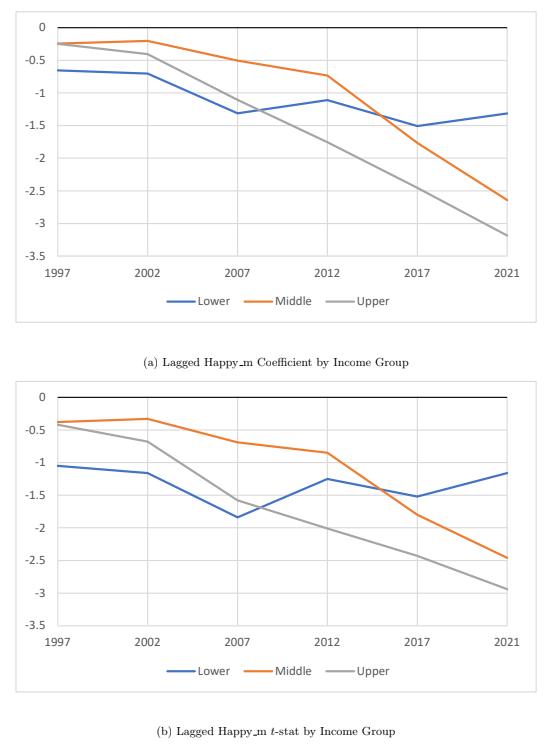
Figure 10: Lagged Happy m by Income Group. This figure plots the estimated lagged Happy coefficients and t-statistics from Equation (6) for each income group, where the regressions are run using a 20-year time window that ends in December of the labeled years. The plot corresponds to the values displayed in Tables 8, 9, and 10.

David Sadka Senior Thesis 2024

David Sadka Understanding Economics through Music Sentiment

Understanding Economics through Music Sentiment