Optimizing Energy Load for an 80 m2 space in Uttarakhand
21/22 ART041 Climate, Comfort and Energy MSc Sustainable Mega-Buildings
By Deepak K Sadhwani February 2022
1
Table of Contents Declaration Form……………………………………………………….…………………………………....…1 Table of Contents…………………………………………………….…………………………………....…...2 List of Figures………………………………………………………….…………………………....................3 1. Introduction………………………………………………………….………………………………….…….4 1.1. Climate and Weather of the chose location………….…………………………………………………4 1.2. The Forrest Essentials Factory Packaging Area……………………………………………………….5 1.3. Thermal envelope specification…………………………………………………………………………..6 1.4. Occupants and space utilization………………………………………………………………………….6 2. Literature………………………………………………………………………………………………………6 3. Methodology…………………………………………………………………………………………………..7 3.1. Weather data………………………………………………………………………………………………..7 3.2. Selection of building and space……………………………………………………………………………7 3.3. Calculation of Energy demand of the base case ………………………………………………………..7 4. Discussion……………………………………………………………………………………………………11 4.1. Current practice & implications…………………………………………………………………………..11 4.2. Best practice……………………………………………………………………………………………….12 5. Conclusions and limitations………………………………………………………………………………...13 5.1. Conclusions………………………………………………………………………………………………..13 5.2. Limitations………………………………………………………………………………………………….13 References……………………………………………………………………………………………………...14 Appendix A. Thermal transmittance values elements of thermal envelope………………………………15 Appendix B. Ventilation & Infiltration rate calculation……………………………………………………….16 Appendix C: Table B.8 of EN 16798-1:2019…………………………………………………………………16 Appendix D. Grasshopper - Ladybug Solar Radiation Definition………………………………………….16 Appendix E: Internal Comfort Temperature calculation for average & extreme conditions…………….17 Appendix F: Heat transfer through conduction………………………………………………………………18 Appendix G: Heat transfer through ventilation………………………………………………………………19 Appendix H: Heat gains through solar radiation…………………………………………………………….19 Appendix I: Solar factor selection……………………………………………………………………………..19 Appendix J: Internal heat gain…………………………………………………………………………………20 Appendix K: Base Case Heat transfer table…………………………………………………………………20 Appendix L: Best Case Heat transfer table………………………………………………………………….20 Appendix M: Best case U values……………………………………………………………………………..21
2
List of Figures
Figure 1. (a) Site location. …….……………….……………………….…...............................................…4 Figure 2. Extreme Weather data ………………………………….…………………………………..............4 Figure 3. Exploded Axonometric view of the workshop space.……………….………………………….....5 Figure 4. Internal comfort temperature graph……………….………………………………………………..7 Figure 5. Heat transfer through conduction graphs.……….…………………………………….…………..8 Figure 6. Heat transfer through ventilation graph.……………………………………………………………9 Figure 7. Heat gain through solar radiation graph.………………………………………………………….10 Figure 8. Heat transfer across all months……………………………………………………………………11 Figure 9. Best case vs Base case heat transfer graph………………………………………………………12
List of Tables
Table 1. Dimensions of the workshop space…………………………………………………………………5 Table 2. Base Case Envelope specifications…………………………………………………………………5 Table 3. Best Case Envelope specifications…………………………………………………………………12
3
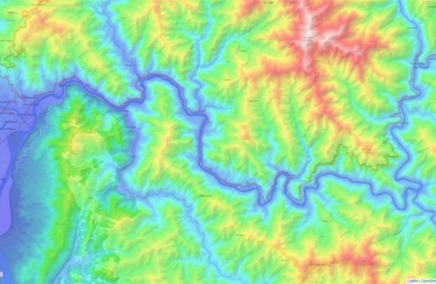
1. Introduction The aim of the paper is to investigate and optimize the Forrest Essentials factory’s workshop area in Uttarakhand in terms of fabric specifications and servicing. The space will be investigated based on heat loss and heat gains during an entire year for average and extreme temperatures. The results will be used to identify problems with fabric and servicing and suggest optimizations to reduce the annual energy demand. 1.1. Climate and Weather of the chose location The space is in Lodsi, Uttarakhand at 682m altitude (Figure 1). The site location falls under ‘Cwb’ region according to the Köppen-Gieger classification matrix (Kottek et al., 2006), depicting temperate climate with dry winters and warm summer.
Project Site
Project Site
(a)
(b)
Figure 1. (a) Site location, (b) Altitude map: Uttarakhand. Source: SolarGIS, ArcGIS
In extreme summers the air temperature ranges from 12 °C to 44 °C. In extreme winters, the air temperature ranges from 1 °C to 33 °C. At its extremes, the location will receive 2350mm precipitation with its peak number of days in July (27 days) and August (26 days). Relative humidity (RH) greater than 90% has been recorded for all the months. The dominant wind direction is North-East (70% of hours) with highest ever recorded wind velocity of 12 meters per second in May (Figure 2).
Figure 2. Extreme Weather data (a) Annual wind wheel, (b) Rainfall data, (c) Daily temperature range. Source: Climate Consultant, Meteonorm
4
1.2. The Forrest Essentials Factory Packaging Area The area of the chosen workshop is 80 square meters with surface to volume ratio of approximately 1. The space is designed to be predominantly free running for its users to conduct light manual work. Workshop space faces North with a Window to wall ratio (WWR) of 70% (Table 1).
Figure 3. Exploded Axonometric view of the workshop space. © Author. Source: SketchUp Table 1. Dimensions of the workshop space. Length 8M
Breadth
Breadth
Surface
Height
Wall Area (sqm)
AreaArea (sqm) Glazing Doors (sqm)
olume
Height 4Mm to 5 M N-S slope External 10
10 M
8m
oof
8m
Length
Area
Volume
80all sqm
337 cum
East
West 4
10 m
Façade North
la ing
5m 4 to South
12
16
Floor
80 s40uare meters 14 -
7
olume
337 cubic meters
all Area
12
la ing Area
40
5
16 14
34
to 5 m
34
meters 80 s uare -
-
-
337 cubic meters
34
34
1.3. Thermal envelope specification Thermal transmittance values for the elements provided by the architecture firm were verified by recalculating each material’s thermal resistance (Appendix A). The U-values ae found to be 1.68 W/(m2K) as against 1.3 W/(m2K) for external walls, 0.27 W/(m 2K) as against 0.25 W/(m 2K) for roof. The U-value for floor (1.90 W/(m 2K)) has been calculated using the same equation. The ventilation flow rate has been calculated to be 2.56 air changes per hour @ 4Pa using Table B.8 of EN 16798-1:2019 (Appendix B). Refer table 2 for other specifications. Table 2. Base Case Envelope specifications. Base Case envelope Parameter
Value
Units
Source
External Wall
1.68
W/(m2K)
Govt. Scotland. 2020
Roof
0.27
W/(m2K)
NBC 2016
Floor
1.90
W/(m2K)
Govt. Scotland. 2020, Author
Glazing U Value
2.80
W/(m2K)
Saint-Gobain 2022
Glazing g Value
0.49
Saint-Gobain 2022
Window Wall Ratio North Elevation Infiltration rate
70%
Author 3
0.6
m /h/m
2
Passivhaus PHPPP
1.4. Occupants and space utilization The area is used as for packaging products with 8 workstations. The space is occupied from 9 am to 5 pm for 5 days per week. There is no active heating or mechanical ventilation system installed. Southern side is predominantly view windows towards the corridor with 2 doors on either side for access. The space is designed for 16 permanent women. The metabolic rate of the occupants associated with light benchwork is 2.1 met (Table 6.2 CIBSE Guide A). The thermal insulation values for garments associated with the location are 0.5 clo in summers and 0.9 clo in winters. There is no applicable equipment associated with the activity. LED Lighting profiles are suspended above the 8 workstations.
2. Literature CIBSE Guide A Environmental Design has been used to derive some base case specifications and occupant comfort ranges. Thermal envelope specifications have been calculated for each element using U values specified in government published sources such as National Building Code of India, 2016, and
overnment of Scotland’s document on table of U-values. Ventilation rates have been
calculated using BS EN 16798-1:2019 (Appendix C). Infiltration rates and glazing specifications have been suggested by Passivhaus standards.
6
3. Methodology 3.1. Weather data The typical year weather file for the nearest major city of Dehradun for 2014 is available on Indian Society of Heating, Refrigerating and Air Conditioning Engineers (ISHRAE). The data has been interpolated on Meteonorm from present, future (2100 at RCP 8.5) periods and highest ever recorded values to calculate extreme conditions. The epw file has been recreated by converting the weather file of Dehradun to CSV and updating it with the extreme data of Lodsi from Metonorm.
3.2. Selection of building and space The space to be analyzed is an existing project by Morphogenesis, New Delhi. The project has been categorized as a naturally ventilated zero energy factory off-grid with high quality construction details. Photovoltaic panels have been utilized to supply the total energy demand. The aim of the paper is to assess whether the energy demand of the building could have been reduced without using renewables.
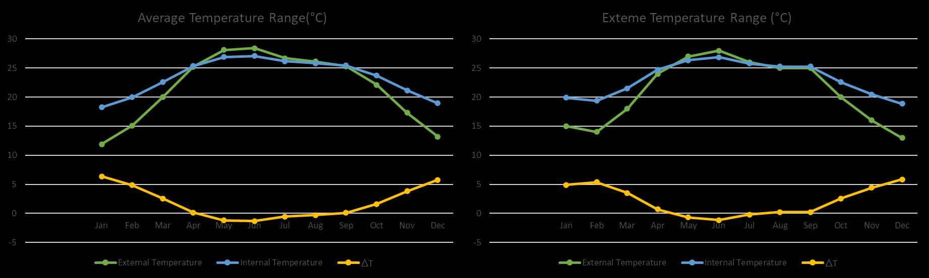
3.3. Calculation of Energy demand of the base case All the calculations are performed at steady state. Internal comfortable temperatures have been calculated for both, average and extreme conditions using adaptive equation for thermal comfort in free-running buildings (Nicol and Humphreys, 2010). 𝑇ei = 11.9+0.534 𝑇𝑜. Refer Appendix E for calculation. where Tei is interior comfort temperature (°C) To is monthly mean/extreme outdoor temperature (°C)
Figure 4. Internal comfort temperature graph. (a) Average temperature range, (b) Extreme temperature range.
Using Figure 3, we observe that Internal comfort temperatures are higher than outdoor temperatures for the summer months of May, June, and July, for both average and extreme conditions. This suggests high gains through the envelope and relatively higher solar gains compared to the other months. Heat transfer through fabric is calculated using the following equation, Qf = ΣUA(To-Tei) where: Qf = heat transfer across the envelope due to conduction; kWh U = thermal transmittance (U-value) of the element; W/(m 2K) A = Surface area of the element; m 2 7
Figure 5. Heat transfer through conduction graphs. (a) Annual Heat Transfer for average and extreme conditions, (b) monthly break-up (c) Break-up of elements for average condition, (b) Break-up of elements for extreme condition.
In average conditions, annual energy demand accounts to ~11,000 kWh (Appendix E). Extreme conditions result in additional 2000 kWh of energy demand. Extreme conditions will therefore be analyzed for heat transfer calculation. Heat transfer through fabric suggests heat loss during the months of September to April. Summer months of May, June and July suggest heat gains. Heat transfer through external wall, floor is higher in average conditions in winter months, whereas extreme conditions state higher energy demand in summer months. Heat transfer through floor accounts for maximum heat transfer across all months. Roof and door have negligible impact on the energy demand. A lower U value for floor, glazing and external wall elements may result in drastic decrease in energy demand.
Heat transfer through ventilation is calculated using the following equation, Qv = nV/3(To-Tei) where: Qv = heat transfer across the envelope due to ventilation and infiltration; kWh n = ventilation flow rate + infiltration rate; ac/h @ 50 Pa V = Volume of the space; m 3 Heat transfer has been calculated for both, occupied and unoccupied hours. Occupied hours are assumed to be naturally ventilated for 9 hours a day and 5 days a week. Unoccupied hours are calculated for the rest of the time when the windows are shut and only infiltration losses take place.
8
Figure 6. Heat transfer through ventilation graph.
The annual heat transfer through ventilation is 1850 kWh (Appendix G). Unoccupied hours amount to 6% of the total energy demand. Summer months of May, June, and July result in heat gains, whereas the remaining months result in heat losses. Heat gains account to 7% of the total energy demand. Heat transfer through solar radiation is calculated using the following equation, Qs = (I x tg x A) where: Qs = heat transfer across the envelope due to solar transmission; kWh tg = g value of glass. A = Area of the space; m 2 I = Irradiance on the surface; kWh/m 2 The building is open to sun from the North. The solar radiation simulations are caried out in Ladybug plugin of Grasshopper using the definition specified in Appendix C targeting the north façade only. The space is assumed to be exposed to capture maximum radiation on façade. Windows are assumed to be double glazed units, air filled with 12mm gap between panes, The solar factor (g-value) has been referenced from manufacturer’s data (Appendix I).
9
Figure 7. Heat gain through solar radiation graph.
Annual heat gains due to solar radiation amount to 123 kWh (Appendix H). Facing north, the space receives sparse heat gains. The maximum being 19.1 kWh in July. A better performing glass with lower solar factor can reduce these gains substantially, if required. Internal heat gains comprise of occupant (Qo) and Lighting (Ql). There are 16 women workers in the space. Therefore, using Table 6.3 CIBSE Guide A, the occupant heat gains (both sensible and latent) amounts to 200 W per women per hour. A factor of 85% has been applied due to the occupants being women. This contributes to 633 kWh per month for 22 working days of 9 hours each. Lighting Heat gains have been calculated using Table 6.2 CIBSE Guide A. The sensible heat gain from lighting has been assumed to be 12W per square meter. Assuming the lighting is switched on during all working hours, heat gains contribute to 211 kWh heat gain per month (Appendix J).
Heat balance is calculated using the following equation. Qf + Qv + Qs + Qo +Ql + Qh + Qc = 0, where: Qh = heat transfer from heating equipment; kWh Qc = heat transfer from cooling equipment; kWh As the space is naturally ventilated, Qh and Qc are assumed to be zero. The heat balance equation is used to calculate the heating and cooling demands of the space specific to each month. (Appendix K)
10
Figure 8. Heat transfer across all months.
Based on the graph of base case heat transfer for the space (Figure 7), an optimization can pe recalculated with better envelope specifications to reduce the energy demand of the space. U value of the floor, external wall and glazing can be enhanced with the aim to balance the heat transfer.
4. Discussion 4.1. Current practice & implications April to September experience net heat gains primarily due internal and thermal envelope specifications. The space will require cooling during these months. The remaining six months experience net heat loss primarily due to thermal envelope and will require heating. The annual energy demand of the building is 15714 kWh annually. Heat transfer due to thermal envelope is maximum. Flooring, glazing, and external walls contribute to most of the demands. Existing external brick wall with stone cladding (U value:1.68 W/(m2K)) can be replaced with better performing elements. Existing roofing can be enhanced by adding cavity and an insulation layer. Flooring RCC Slab with U value of 1.81 W/(m 2K) can be replaced with a better performing alternative. Double Glazing can be replaced with Triple Glazing with low e argon filled to reduce heat transfer. Blinds can be utilized to reduce heat gains during summer months. The envelope performs well against convective heat transfers, so no further optimizations have been suggested. However, a higher surface to volume ratio will result in reduced energy demands. Heat gain through solar is negligible. Changing the orientation will result in increased energy demand. Sun shading is not required for the purpose of energy demand but can be added to protect the space from rain. Glazing area can be further increased for better views. Slightly better performing lighting fixtures can be utilized with heat gain of 10W per square meter. Further limiting the use of artificial lighting and relying on natural light during morning and afternoon will reduce the energy demand. 11
4.2. Best practice Table 3 highlights the optimizations in thermal envelope. To optimize heat transfer through conduction, external wall has been replaced with 200mm AAC blocks, 200mm mud brick wall, mineral wool insulation and a 10mm cavity. Cladding and plastering stays the same as base case. For roof, internal liner has been replaced with timber, and stone wool insulation is replaced with mineral wool. Flooring has been changed from 150mm RCC to 200mm Cellular concrete with specific heat capacity of 1.05 kJ/kgK. The inner glass of the existing glazing unit has been replaced with a triple glazed insulated unit. The pane is replaced by PPC insulated metal top panel and timber frame to provide structural support. Outer glass stays the same. Refer Appendix N for revised envelope calculations. Table 3. Best Case Envelope specifications. Best practice envelope Parameter
Value
Units
Source
External Wall
0.25
W/(m2K)
NBC2016, Author
Roof
0.16
W/(m2K)
NBC2016, Author
Floor
0.81
W/(m2K)
NBC2016, Author
Glazing U Value
0.58
W/(m2K)
Saint-Gobain 2022
Glazing g Value
0.52
Saint-Gobain 2022
WWR North Elevation
95%
Author
The annual energy demand reduces to 4853 kWh, which is an improvement of 70% from the base case scenario (Appendix M). Figure 8 shows the improvement of the space after applying the abovementioned replacements. January and November are observed to be in a state of heat balance. Negligible heating losses are observed for February and December. Heating is required during these months. Heat gains are observed from March to October contributing to 4000kWh cooling energy demand.
Figure 9. Best case vs Base case heat transfer graph.
12
5. Conclusions and limitations 5.1. Conclusions Base case scenario showed higher energy demands (>1000 kWh) for 8 months. Best practices brough this down to all months utilizing less than 1000kWh with 2 months observed to be in a state of heat balance. This optimized cooling demand may be eliminated by utilizing natural ventilation solely. The user can control the cooling needed for the space. Thus, making the space net zero on energy demand. The key factor of the optimizations was the thermal envelope of the space. Changes in U values eliminated maximum energy demands. Other criteria such as infiltration losses would have had major implications on the calculations if the space was not assumed to be airtight.
5.2. Limitations The calculations were performed in steady state conditions and thus, conclude with a broader idea on the assumed space. A detailed dynamic state condition is more suitable for an existing space. Effects of thermal mass can also be considered to understand the space better.
13
References [1] BS EN 16798-1:2019 - Energy performance of buildings - Ventilation for buildings. 2019: BSI Standards [2] CIBSE Guide A - Environmental Design (7th Edition). 2015: CIBSE.
[3]Database.passivehouse.com.
2022. List
of
windows.
Available
at:
https://database.passivehouse.com/en/components/list/window?lat=51.4567&lon=-3.3434&cz=4.
[4] Nicol, F. and Humphreys, M., 2010. Derivation of the adaptive equations for thermal comfort in freerunning buildings in European standard EN15251. Building and Environment, 45(1), pp.11-17.
[5] Gov.scot. 2022. U Values: guidance. [online] Available at: https://www.gov.scot/publications/tablesof-u-values-and-thermal-conductivity/.
[6] Kottek, M., Grieser, J., Beck, C., Rudolf, B. and Rubel, F., 2006. World Map of the Köppen-Geiger climate classification updated. Meteorologische Zeitschrift, 15(3), pp.259-263.
[7] National building code of India 2016. 2nd ed.
[8[ Natural Stone Institute. 2022. What Natural Stone is best for heated surfaces. [online] Available at: https://www.naturalstoneinstitute.org/stoneprofessionals/technical-bulletins/rvalue/.
[9] Saint-gobain-facade-glass.com. 2022. Product Performance Tables | Saint-Gobain Façade. [online] Available
at:
https://www.saint-gobain-facade-glass.com/specification-tools/product-performance-
tables.
[10] Weather.whiteboxtechnologies.com. 2022. Select ISHRAE Weather Files. [online] Available at: http://weather.whiteboxtechnologies.com/ISHRAE.
[11] Zeng, T., Jiang, H. and Hao, F., 2022. Study on the effect of aluminium foil on packaging thermal insulation performance in cold chain logistics. Packaging Technology and Science.
14
Appendix A. Thermal transmittance values elements of thermal envelope. External wall Element
Thickness [m]
External surface resistance Limestone cladding
0.15
Brickwork Mud Plaster
0.23 0.015
K-value [W/(mk)]
Resistance [m2K/W]
Source
1.33
0.04 0.11
WSA, Energy & Heat Natural Stone Institute
0.84 0.4
0.27 0.04
WSA, Energy & Heat NBC 2016
0.13 0.59 1.68
WSA, Energy & Heat
Internal surface resistance Total thermal resistance U Value
W/(m2K)
Roof Element
Thickness [m]
K-value [W/(mk)]
External surface resistance
Resistance [m2K/W]
Source
0.04
WSA, Energy & Heat
External Aluminium Sheet
0.0009
247
0.00
NBC 2016
Stone wool Aluminium Foil Internal Liner Sheet
0.1
0.04
0.0006
247
2.50 1.00 0.00
NBC 2016 Zeng et. al NBC 2016
0.10 3.64 0.27
WSA, Energy & Heat
Internal surface resistance Total thermal resistance U Value
W/(m2K)
Floor Element Internal surface resistance RCC slab Screed Total thermal resistance
Thickness [m] 0.15 0.1
K-value [W/(mk)] 1.35 0.41
U Value Floor Element
Thickness [m]
K-value [W/(mk)]
Resistance [m2K/W]
Source
0.17 0.11 0.24 0.53
WSA, Energy & Heat Govt. Scotland. 2020 Govt. Scotland. 2020
1.90
W/(m2K)
Resistance [m2K/W]
Source
Internal surface resistance RCC slab
0.3
1.3
0.17 0.23
WSA, Energy & Heat NBC 2016
Steel
0.05
50
0.001
NBC 2016
0.40 2.49
W/(m2K)
Total thermal resistance U Value Glazing Element Double glazed Steel Sections with
Thickness [m]
K-value [W/(mk)]
Source Govt. Scotland. 2020
0.1
U Value g Value Door Element
Resistance [m2K/W]
2.80 0.49 Thickness [m]
K-value [W/(mk)]
Solid Timber U Value
Resistance [m2K/W]
3.00
15
Saint Gobain
Source Govt. Scotland. 2020 W/(m2K)
Appendix B. Ventilation & Infiltration rate calculation No. of occupants Volume Airflow per person Airflow total
Flow rate Infiltration rate Infiltration rate Ventilation+ Infiltration rate
16 337 10 240 0.24 864 2.56 0.60 0.06 2.62
l l/s/ person l/s m3/s m3 ac/h @5 Pa ac/h @50 Pa
Appendix C: Table B.8 of EN 16798-1:2019
Appendix D. Grasshopper - Ladybug Solar Radiation Definition
16
Appendix E: Internal Comfort Temperature calculation for average & extreme conditions Table 1. Average conditions Month
External Temperature (°C)
Adaptive Equation
Thermal
Comfort
Internal Temperature (°C)
ᐃT (°C)
Jan
15
𝑇𝑐=11.9+0.534 𝑇𝑜
19.9
4.9
Feb
14
𝑇𝑐=11.9+0.534 𝑇𝑜
19.4
5.4
Mar
18
𝑇𝑐=11.9+0.534 𝑇𝑜
21.5
3.5
Apr
24
𝑇𝑐=11.9+0.534 𝑇𝑜
24.7
0.7
May
27
𝑇𝑐=11.9+0.534 𝑇𝑜
26.3
-0.7
Jun
28
𝑇𝑐=11.9+0.534 𝑇𝑜
26.9
-1.1
Jul
26
𝑇𝑐=11.9+0.534 𝑇𝑜
25.8
-0.2
Aug
25
𝑇𝑐=11.9+0.534 𝑇𝑜
25.3
0.3
Sep
25
𝑇𝑐=11.9+0.534 𝑇𝑜
25.3
0.3
Oct
20
𝑇𝑐=11.9+0.534 𝑇𝑜
22.6
2.6
Nov
16
𝑇𝑐=11.9+0.534 𝑇𝑜
20.4
4.4
Dec
13
𝑇𝑐=11.9+0.534 𝑇𝑜
18.8
5.8
Table 2. Extreme conditions Month
External Temperature
Adaptive Equation
Thermal
Jan
11.9
𝑇𝑐=11.9+0.534 𝑇𝑜
18.3
6.4
Feb
15.1
𝑇𝑐=11.9+0.534 𝑇𝑜
20.0
4.9
Mar
20
𝑇𝑐=11.9+0.534 𝑇𝑜
22.6
2.6
Apr
25.2
𝑇𝑐=11.9+0.534 𝑇𝑜
25.4
0.2
May
28.1
𝑇𝑐=11.9+0.534 𝑇𝑜
26.9
-1.2
Jun
28.4
𝑇𝑐=11.9+0.534 𝑇𝑜
27.1
-1.3
Jul
26.7
𝑇𝑐=11.9+0.534 𝑇𝑜
26.2
-0.5
Aug
26.1
𝑇𝑐=11.9+0.534 𝑇𝑜
25.8
-0.3
Sep
25.3
𝑇𝑐=11.9+0.534 𝑇𝑜
25.4
0.1
Oct
22.1
𝑇𝑐=11.9+0.534 𝑇𝑜
23.7
1.6
Nov
17.3
𝑇𝑐=11.9+0.534 𝑇𝑜
21.1
3.8
Dec
13.2
𝑇𝑐=11.9+0.534 𝑇𝑜
18.9
5.7
17
Comfort
Internal Temperature
ᐃT
18
4.9
2.6
0.2
-1.2
-1.3
-0.5
-0.3
0.1
1.6
3.8
5.7
Mar
Apr
May
Jun
Jul
Aug
Sep
Oct
Nov
Dec
1.68
1.68
1.68
1.68
1.68
1.68
1.68
1.68
1.68
1.68
1.68
1.68
U Value W/(sqm. K)
4.9
5.4
3.5
0.7
-0.7
-1.1
-0.2
0.3
0.3
2.6
4.4
5.8
Jan
Mar
Apr
May
Jun
Jul
Aug
Sep
Oct
Nov
Dec
ᐃT
Feb
Month
80
80
80
80
80
80
80
80
80
80
80
80
346
92
60
26
2
-4
-9
-21
-19
2
41
73
102
4.25
4.25
4.25
4.25
4.25
4.25
4.25
4.25
4.25
4.25
4.25
4.25
1.68
1.68
1.68
1.68
1.68
1.68
1.68
1.68
1.68
1.68
1.68
1.68
96
96
96
96
96
96
96
96
96
96
96
96
3048
702
517
310
30
29
-26
-134
-82
83
422
605
590
0.27
0.27
0.27
0.27
0.27
0.27
0.27
0.27
0.27
0.27
0.27
80
80
80
80
80
80
80
80
80
80
80
80
407
94
69
41
4
4
-3
-18
-11
11
56
81
79
4.25
4.25
4.25
4.25
4.25
4.25
4.25
4.25
4.25
4.25
4.25
4.25
0.27
0.27
0.27
0.27
0.27
0.27
0.27
0.27
0.27
0.27
0.27
0.27
5446
1454
940
405
28
-64
-137
-327
-302
38
653
1151
1607
2.80
2.80
2.80
2.80
2.80
2.80
2.80
2.80
2.80
2.80
2.80
2.80
U Value W/(sqm. K)
54
54
54
54
54
54
54
54
54
54
54
54
2422
647
418
180
12
-29
-61
-145
-134
17
290
512
715
3.00
3.00
3.00
3.00
3.00
3.00
3.00
3.00
3.00
3.00
3.00
3.00
Glazing Area Heat Transfer U Value sqm kWh W/(sqm. K)
7
7
7
7
7
7
7
7
7
7
7
7
336
90
58
25
80
80
80
80
80
80
80
80
80
80
80
80
6412
1478
1088
653
63
61
-55
-281
-173
175
888
1272
1242
2.80
2.80
2.80
2.80
2.80
2.80
2.80
2.80
2.80
2.80
2.80
2.80
54
54
54
54
54
54
54
54
54
54
54
54
2852
657
484
290
28
27
-24
-125
-77
78
395
566
552
3.00
3.00
3.00
3.00
3.00
3.00
3.00
3.00
3.00
3.00
3.00
3.00
7
7
7
7
7
7
7
7
7
7
7
7
2
-4
-8
-20
-19
2
40
71
99
Doors Area Heat Transfer sqm kWh
2974
1922
829
57
-131
-281
-668
-618
79
1335
2354
3288
3022
13115
2225
1335
129
125
-112
-575
-353
358
1817
2602
2540
396
Total Fabric Heat Transfer (kWh)
11138
Total Fabric Heat Transfer (kWh)
91
67
40
4
4
-3
-17
-11
11
55
79
77
Doors Glazing Floor Area Heat Transfer Area Heat TransferU Value Area Heat Transfer U Value kWh kWh W/(sqm. K) sqm sqm kWh W/(sqm. K) sqm
80
80
80
80
80
80
80
80
80
80
80
80
Floor Area Heat Transfer sqm kWh
0.27
2588
691
447
193
13
-31
-65
-155
-144
18
310
547
764
Roof Area Heat Transfer U Value sqm kWh W/(sqm. K)
Roof Area Heat TransferU Value kWh W/(sqm. K) sqm
96
96
96
96
96
96
96
96
96
96
96
96
External Wall Area Heat Transfer U Value sqm kWh W/(sqm. K)
External Wall Area Heat TransferU Value U Value kWh W/(sqm. K) sqm W/(sqm. K)
Table 1. Average conditions
6.4
Jan
ᐃT
Feb
Month
Table 1. Average conditions
APPENDIX F: Heat transfer through conduction
Appendix G: Heat transfer through ventilation Table 1. Annual heat transfer through ventilation Month
ᐃT
Occupied hours
Ventilation heat transfer Unoccupied hours kWh
Total
Jan
4.9
287
17
304
Feb
5.4
314
19
333
Mar
3.5
205
12
217
Apr
0.7
42
3
44
May
-0.7
-40
-2
-42
Jun
-1.1
-67
-4
-71
Jul
-0.2
-13
-1
-13
Aug
0.3
15
1
15
Sep
0.3
15
1
15
Oct
2.6
151
9
160
Nov
4.4
259
16
275
Dec
5.8
341
21
361
1599
Appendix H: Heat gains through solar radiation Table 1. Annual heat gains through solar radiation
Solar Irradiance kWh/m2
Month
Area m2
g value kWh
Jan
0.3
40.0
0.5
6.1
Feb
0.3
40.0
0.5
6.7
Mar
0.5
40.0
0.5
9.3
Apr
0.5
40.0
0.5
9.8
May
0.7
40.0
0.5
12.7
Jun
0.9
40.0
0.5
16.7
Jul
1.0
40.0
0.5
19.1
Aug
0.8
40.0
0.5
15.7
Sep
0.5
40.0
0.5
9.8
Oct
0.3
40.0
0.5
6.4
Nov
0.3
40.0
0.5
5.4
Dec
0.3
40.0
0.5
4.9
Appendix I: Solar factor selection Table 1. Selection of solar factor of gla ing using Saint
obain’s product performance table.
19
Appendix J: Internal heat gain Table 1. Annual internal heat gains.
Occupant
Lighting
Month
W
Nos
kWh
W
sqm
kWh
Jan
200
16
633
12.0
80.0
211
Feb
200
16
633
12.0
80.0
211
Mar
200
16
633
12.0
80.0
211
Apr
200
16
633
12.0
80.0
211
May
200
16
633
12.0
80.0
211
Jun
200
16
633
12.0
80.0
211
Jul
200
16
633
12.0
80.0
211
Aug
200
16
633
12.0
80.0
211
Sep
200
16
633
12.0
80.0
211
Oct
200
16
633
12.0
80.0
211
Nov
200
16
633
12.0
80.0
211
Dec
200
16
633
12.0
80.0
211
Appendix K: Base Case Heat transfer table Total Fabric
Ventilation heat transfer kWh
Month
kWh
Solar Occupant Lighting Heat Gain Heat Gain Heat Gain kWh kWh kWh
Jan
2540
304
6.1
633
211
Feb
2602
333
6.7
633
211
Mar
1817
217
9.3
633
211
Apr
358
44
9.8
633
211
May
-353
-42
12.7
633
211
Jun
-575
-71
16.7
633
211
Jul
-112
-13
19.1
633
211
Aug
125
15
15.7
633
211
Sep
129
15
9.8
633
211
Oct
1335
160
6.4
633
211
Nov
2225
275
5.4
633
211
Dec
3022
361
4.9
633
211
Net Result kWh 1994 2084 1181 -451 -1252 -1506 -988 -719 -709 644 1651 2535 15714
Description Heat Loss Heat Loss Heat Loss Heat Gain Heat Gain Heat Gain Heat Gain Heat Gain Heat Gain Heat Loss Heat Loss Heat Loss
Inference Heating required Heating required Heating required Cooling required Cooling required Cooling required Cooling required Cooling required Cooling required Heating required Heating required Heating required
Appendix L: Best Case Heat transfer table Total Fabric
Ventilation heat transfer kWh
Month
kWh
Solar Occupant Lighting Heat Gain Heat Gain Heat Gain kWh kWh kWh
Jan
462
304
3.3
633
48
Feb
477
333
3.3
633
48
Mar
330
217
3.3
633
48
Apr
65
44
3.3
633
48
May
-64
-42
3.3
633
48
Jun
-105
-71
3.3
633
48
Jul
-20
-13
3.3
633
48
Aug
23
15
3.3
633
48
Sep
24
15
3.3
633
48
Oct
243
160
3.3
633
48
Nov
406
275
3.3
633
48
Dec
549
361
3.3
633
48
20
Net Result kWh 82 126 -136 -574 -790 -860 -717 -645 -645 -281 -2 227
Description Heat Balance Heat Loss Heat Gain Heat Gain Heat Gain Heat Gain Heat Gain Heat Gain Heat Gain Heat Gain Heat Balance Heat Loss
Inference No energy demands Heating required Cooling required Cooling required Cooling required Cooling required Cooling required Cooling required Cooling required Cooling required No energy demands Heating required
APPENDIX M: Best case U values External wall Element
Thickness [m]
K-value [W/(mk)]
Resistance [m2K/W]
External surface resistance Limestone cladding AAC
0.04 0.15
1.33
0.11
0.2
0.089
2.25
Cavity
0.01
Mineral Wool
0.03
0.03
1.00
0.2
0.75
0.27
0.015
0.4
0.04
Mud brick Mud Plaster
0.15
Internal surface resistance
0.13
Total thermal resistance
3.98
U Value
0.25 Roof Element
Thickness [m]
K-value [W/(mk)]
Resistance [m2K/W]
External surface resistance
0.04
GI Sheet
0.1
0.5
0.20
Mineral wool
0.1
0.03
3.33
Aluminium Foil Internal Timber
1.00 0.1
0.072
1.39
Internal surface resistance
0.10
Total thermal resistance
6.06
U Value
0.16 Floor Element
Thickness [m]
K-value [W/(mk)]
Resistance [m2K/W]
Internal surface resistance Cellular concrete
0.17 0.2
0.188
1.06
Total thermal resistance
1.23
U Value
0.81 Glazing Element
Thickness [m]
K-value [W/(mk)]
Resistance
Double glazed Steel Sections with
0.1
U Value
0.58 W/(m2K)
g value
0.52 Door Element
Thickness [m]
K-value [W/(mk)]
Resistance [m2K/W]
Solid Timber U Value
1.23
21