Instant download Python deep learning: understand how deep neural networks work and apply them to re
Visit to download the full and correct content document: https://ebookmass.com/product/python-deep-learning-understand-how-deep-neural-n etworks-work-and-apply-them-to-real-world-tasks-3rd-edition-vasilev/
More products digital (pdf, epub, mobi) instant download maybe you interests ...
AI Applications to Communications and Information Technologies: The Role of Ultra Deep Neural Networks
All rights reserved. No part of this book may be reproduced, stored in a retrieval system, or transmitted in any form or by any means, without the prior written permission of the publisher, except in the case of brief quotations embedded in critical articles or reviews.
Every effort has been made in the preparation of this book to ensure the accuracy of the information presented. However, the information contained in this book is sold without warranty, either express or implied. Neither the author, nor Packt Publishing or its dealers and distributors, will be held liable for any damages caused or alleged to have been caused directly or indirectly by this book.
Packt Publishing has endeavored to provide trademark information about all of the companies and products mentioned in this book by the appropriate use of capitals. However, Packt Publishing cannot guarantee the accuracy of this information.
Associate Group Product Manager: Niranjan Naikwadi
Ivan Vasilev started working on the first open source Java deep learning library with GPU support in 2013. The library was acquired by a German company, with whom he continued its development. He has also worked as a machine learning engineer and researcher in medical image classification and segmentation with deep neural networks. Since 2017, he has focused on financial machine learning. He co-founded an algorithmic trading company, where he’s the lead engineer.
He holds an MSc in artificial intelligence from Sofia University St. Kliment Ohridski and has written two previous books on the same topic.
About the reviewer
Krishnan Raghavan is an IT professional with over 20+ years of experience in the areas of software development and delivery excellence, across multiple domains and technologies, ranging from C++ to Java, Python, Angular, Golang, and data warehousing.
When not working, Krishnan likes to spend time with his wife and daughter, besides reading fiction, nonfiction, and technical books and participating in hackathons. Krishnan tries to give back to the community by being part of a GDG, the Pune volunteer group, helping the team to organize events.
You can connect with Krishnan at mailtokrishnan@gmail.com or via LinkedIn at www.linkedin.com/in/krishnan-Raghavan
I would like to thank my wife, Anita, and daughter, Ananya, for giving me the time and space to review this book.
Part 1: Introduction to Neural Networks
Part 2: Deep Neural Networks for Computer Vision
Part 4: Developing and Deploying Deep Neural Networks
Preface
The book will start from the theoretical foundations of deep neural networks (NN), and it will delve into the most popular network architectures – transformers, transformer-based large language models (LLMs), and convolutional networks. It will introduce these models in the context of various computer vision and natural language processing (NLP) examples, including state-of-the-art applications such as text-to-image generation and chatbots.
Each chapter is organized with a comprehensive theoretical introduction to the topic as its main body. This is followed by coding examples that serve to validate the presented theory, providing readers with practical hands-on experience. The examples are executed using PyTorch, Keras, or Hugging Face Transformers.
Who this book is for
This book is for individuals already familiar with programming – software developers/engineers, students, data scientists, data analysts, machine learning engineers, statisticians, and anyone interested in deep learning who has Python programming experience. It is designed for people with minimal prior deep learning knowledge, employing clear and straightforward language throughout.
What this book covers
Chapter 1, Machine Learning – an Introduction, discusses the basic machine learning paradigms. It will explore various machine learning algorithms and introduce the first NN, implemented with PyTorch.
Chapter 2, Neural Networks, starts by introducing the mathematical branches related to NNs – linear algebra, probability, and differential calculus. It will focus on the building blocks and structure of NNs. It will also discuss how to train NNs with gradient descent and backpropagation.
Chapter 3, Deep Learning Fundamentals, introduces the basic paradigms of deep learning. It will make the transition from classic networks to deep NNs. It will outline the challenges of developing and using deep networks, and it will discuss how to solve them.
Chapter 4, Computer Vision with Convolutional Networks, introduces convolutional networks – the main network architecture for computer vision applications. It will discuss in detail their properties and building blocks. It will also introduce the most popular convolutional network models in use today.
Chapter 5, Advanced Computer Vision Applications, discusses applying convolutional networks for advanced computer vision tasks – object detection and image segmentation. It will also explore using NNs to generate new images.
Chapter 6, Natural Language Processing and Recurrent Neural Networks, introduces the main paradigms and data processing pipeline of NLP. It will also explore recurrent NNs and their two most popular variants – long short-term memory and gated recurrent units.
Chapter 7, The Attention Mechanism and Transformers, introduces one of the most significant recent deep learning advances – the attention mechanism and the transformer model based around it.
Chapter 8, Exploring Large Language Models in Depth, introduces transformer-based LLMs. It will discuss their properties and what makes them different than other NN models. It will also introduce the Hugging Face Transformers library.
Chapter 9, Advanced Applications of Large Language Models, discusses using LLMs for computer vision tasks. It will focus on classic tasks such as image classification and object detection, but it will also explore state-of-the-art applications such as text-to-image generation. It will introduce the LangChain framework for LLM-driven application development.
Chapter 10, Machine Learning Operations (MLOps), will introduce various libraries and techniques for easier development and production deployment of NN models.
To get the most out of this book
Many code examples in the book require the presence of a GPU. Don’t worry if you don’t have one. To avoid any hardware limitations, all code examples are available as Jupyter notebooks, executed on Google Colab. So, even if your hardware is not sufficient to run the examples, you can still run them under Colab.
Software/hardware covered in the book Operating system requirements
PyTorch 2.0.1
TensorFlow 2.13
Windows, macOS, or Linux
Windows (legacy support), macOS, or Linux
Hugging Face Transformers 4.33 Windows, macOS, or Linux
Some code examples in the book may use additional packages not listed in the table. You can see the full list (with versions) in the requirements.txt file in the book’s GitHub repo.
If you are using the digital version of this book, we advise you to type the code yourself or access the code from the book’s GitHub repository (a link is available in the next section). Doing so will help you avoid any potential errors related to the copying and pasting of code.
Download the example code files
You can download the example code files for this book from GitHub at https://github.com/ PacktPublishing/Python-Deep-Learning-Third-Edition/. If there’s an update to the code, it will be updated in the GitHub repository.
We also have other code bundles from our rich catalog of books and videos available at https:// github.com/PacktPublishing/. Check them out!
Conventions used
There are a number of text conventions used throughout this book.
Code in text: Indicates code words in text, database table names, folder names, filenames, file extensions, pathnames, dummy URLs, user input, and Twitter handles. Here is an example: “Use opencv-python to read the RGB image located at image_file_path.”
A block of code is set as follows:
def build_fe_model():
""""Create feature extraction model from the pre-trained model ResNet50V2"""
# create the pre-trained part of the network, excluding FC layers base_model = tf.keras.applications.MobileNetV3Small(
Any command-line input or output is written as follows:
import tensorflow.keras
When we wish to draw your attention to a particular part of a code block, the relevant lines or items are set in bold:
General feedback: If you have questions about any aspect of this book, email us at customercare@ packtpub.com and mention the book title in the subject of your message.
Errata: Although we have taken every care to ensure the accuracy of our content, mistakes do happen. If you have found a mistake in this book, we would be grateful if you would report this to us. Please visit www.packtpub.com/support/errata and fill in the form.
Piracy: If you come across any illegal copies of our works in any form on the internet, we would be grateful if you would provide us with the location address or website name. Please contact us at copyright@packt.com with a link to the material.
If you are interested in becoming an author: If there is a topic that you have expertise in and you are interested in either writing or contributing to a book, please visit authors.packtpub.com.
Share Your Thoughts
Once you’ve read Python Deep Learning, Third Edition, we’d love to hear your thoughts! Please click here to go straight to the Amazon review page for this book and share your feedback.
Your review is important to us and the tech community and will help us make sure we’re delivering excellent quality content.
Download a free PDF copy of this book
Thanks for purchasing this book!
Do you like to read on the go but are unable to carry your print books everywhere?
Is your eBook purchase not compatible with the device of your choice?
Don’t worry, now with every Packt book you get a DRM-free PDF version of that book at no cost.
Read anywhere, any place, on any device. Search, copy, and paste code from your favorite technical books directly into your application.
The perks don’t stop there, you can get exclusive access to discounts, newsletters, and great free content in your inbox daily
Follow these simple steps to get the benefits:
1. Scan the QR code or visit the link below
https://packt.link/free-ebook/9781837638505
2. Submit your proof of purchase
3. That’s it! We’ll send your free PDF and other benefits to your email directly
Part 1: Introduction to Neural Networks
We’ll start this part by introducing you to basic machine learning theory and concepts. Then, we’ll follow with a thorough introduction to neural networks – a special type of machine learning algorithm.
We’ll discuss the mathematical principles behind them and learn how to train them. Finally, we’ll make the transition from shallow to deep networks.
This part has the following chapters:
• Chapter 1, Machine Learning – an Introduction
• Chapter 2, Neural Networks
• Chapter 3, Deep Learning Fundamentals
1
Machine Learning – an Introduction
Machine learning (ML) techniques are being applied in a variety of fields, and data scientists are being sought after in many different industries. With ML, we identify the processes through which we gain knowledge that is not readily apparent from data to make decisions. Applications of ML techniques may vary greatly and are found in disciplines as diverse as medicine, finance, and advertising.
In this chapter, we’ll present different ML approaches, techniques, and some of their applications to real-world problems, and we’ll also introduce one of the major open source packages available in Python for ML, PyTorch. This will lay the foundation for later chapters in which we’ll focus on a particular type of ML approach using neural networks (NNs). In particular, we will focus on deep learning (DL). DL makes use of more advanced NNs than those used previously. This is not only a result of recent developments in the theory but also advancements in computer hardware. This chapter will summarize what ML is and what it can do, preparing you to better understand how DL differentiates itself from popular traditional ML techniques.
In this chapter, we’re going to cover the following main topics:
• Introduction to ML
• Different ML approaches
• Neural networks
• Introduction to PyTorch
Technical requirements
We’ll implement the example in this chapter using Python and PyTorch. If you don’t have an environment set up with these tools, fret not – the example is available as a Jupyter notebook on Google Colab. You can find the code examples in the book’s GitHub repository: https://github. com/PacktPublishing/Python-Deep-Learning-Third-Edition/tree/main/ Chapter01.
Introduction to ML
ML is often associated with terms such as big data and artificial intelligence (AI). However, both are quite different from ML. To understand what ML is and why it’s useful, it’s important to understand what big data is and how ML applies to it.
Big data is a term used to describe huge datasets that are created as the result of large increases in data that is gathered and stored. For example, this may be through cameras, sensors, or internet social sites.
How much data do we create daily?
It’s estimated that Google alone processes over 20 petabytes of information per day, and this number is only going to increase. A few years ago, Forbes estimated that every day, 2.5 quintillion bytes of data are created and that 90% of all the data in the world has been created in the last two years.
Humans alone are unable to grasp, let alone analyze, such huge amounts of data, and ML techniques are used to make sense of these very large datasets. ML is the tool that’s used for large-scale data processing. It is well suited to complex datasets that have huge numbers of variables and features. One of the strengths of many ML techniques, and DL in particular, is that they perform best when used on large datasets, thus improving their analytic and predictive power. In other words, ML techniques, and DL NNs in particular, learn best when they can access large datasets where they can discover patterns and regularities hidden in the data.
On the other hand, ML’s predictive ability can be successfully adapted to AI systems. ML can be thought of as the brain of an AI system. AI can be defined (though this definition may not be unique) as a system that can interact with its environment. Also, AI machines are endowed with sensors that enable them to know the environment they are in and tools with which they can relate to the environment. Therefore, ML is the brain that allows the machine to analyze the data ingested through its sensors to formulate an appropriate answer. A simple example is Siri on an iPhone. Siri hears the command through its microphone and outputs an answer through its speakers or its display, but to do so, it needs to understand what it’s being told. Similarly, driverless cars will be equipped with cameras, GPS systems, sonars, and LiDAR, but all this information needs to be processed to provide a correct answer. This may include whether to accelerate, brake, or turn. ML is the information-processing method that leads to the answer.
We’ve explained what ML is, but what about DL? For now, let’s just say that DL is a subfield of ML. DL methods share some special common features. The most popular representatives of such methods are deep NNs.
Different ML approaches
As we have seen, the term ML is used in a very general way and refers to the general techniques that are used to extrapolate patterns from large sets, or it is the ability to make predictions on new data based on what is learned by analyzing available known data. ML techniques can roughly be divided into two core classes, while one more class is often added. Here are the classes:
• Supervised learning
• Unsupervised learning
• Reinforcement learning
Let’s take a closer look.
Supervised learning
Supervised learning algorithms are a class of ML algorithms that use previously labeled data to learn its features, so they can classify similar but unlabeled data. Let’s use an example to understand this concept better.
Let’s assume that a user receives many emails every day, some of which are important business emails and some of which are unsolicited junk emails, also known as spam. A supervised machine algorithm will be presented with a large body of emails that have already been labeled by a teacher as spam or not spam (this is called training data). For each sample, the machine will try to predict whether the email is spam or not, and it will compare the prediction with the original target label. If the prediction differs from the target, the machine will adjust its internal parameters in such a way that the next time it encounters this sample, it will classify it correctly. Conversely, if the prediction is correct, the parameters will stay the same. The more training data we feed to the algorithm, the better it becomes (this rule has caveats, as we’ll see next).
In the example we used, the emails had only two classes (spam or not spam), but the same principles apply to tasks with arbitrary numbers of classes (or categories). For example, Gmail, the free email service by Google, allows the user to select up to five categories, which are labeled as follows:
• Primary: Includes person-to-person conversations
• Promotions: Includes marketing emails, offers, and discounts
• Social: Includes messages from social networks and media-sharing sites
• Updates: Includes bills, bank statements, and receipts
• Forums: Includes messages from online groups and mailing lists
To summarize, the ML task, which maps a set of input values to a finite number of classes, is called classification.
In some cases, the outcome may not necessarily be discrete, and we may not have a finite number of classes to classify our data into. For example, we may try to predict the life expectancy of a group of people based on their predetermined health parameters. In this case, the outcome is a numerical value, and we don’t talk about classification but rather regression.
One way to think of supervised learning is to imagine we are building a function, f, defined over a dataset, which comprises information organized by features. In the case of email classification, the features can be specific words that may appear more frequently than others in spam emails. The use of explicit sex-related words will most likely identify a spam email rather than a business/work email. On the contrary, words such as meeting, business, or presentation are more likely to describe a work email. If we have access to metadata, we may also use the sender’s information as a feature. Each email will then have an associated set of features, and each feature will have a value (in this case, how many times the specific word is present in the email’s body). The ML algorithm will then seek to map those values to a discrete range that represents the set of classes, or a real value in the case of regression. The definition of the f function is as follows:
f : space of features → classes = (discrete values or real values)
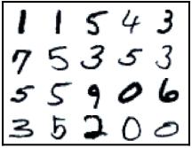
In later chapters, we’ll see several examples of either classification or regression problems. One such problem we’ll discuss is classifying handwritten digits of the Modified National Institute of Standards and Technology (MNIST) database (http://yann.lecun.com/exdb/mnist/). When given a set of images representing 0 to 9, the ML algorithm will try to classify each image in one of the 10 classes, wherein each class corresponds to one of the 10 digits. Each image is 28×28 (= 784) pixels in size. If we think of each pixel as one feature, then the algorithm will use a 784-dimensional feature space to classify the digits.
The following figure depicts the handwritten digits from the MNIST dataset:
Figure 1.1 – An example of handwritten digits from the MNIST dataset
In the next sections, we’ll talk about some of the most popular classical supervised algorithms. The following is by no means an exhaustive list or a thorough description of each ML method. We recommend referring to the book Python Machine Learning, by Sebastian Raschka (https://www.packtpub.
com/product/python-machine-learning-third-edition/9781789955750). It’s a simple review meant to provide you with a flavor of the different ML techniques in Python.
Linear and logistic regression
A regression algorithm is a type of supervised algorithm that uses features of the input data to predict a numeric value, such as the cost of a house, given certain features, such as size, age, number of bathrooms, number of floors, and location. Regression analysis tries to find the value of the parameters for the function that best fits an input dataset.
In a linear regression algorithm, the goal is to minimize a cost function by finding appropriate parameters for the function over the input data that best approximates the target values. A cost function is a function of the error – that is, how far we are from getting a correct result. A popular cost function is the mean squared error (MSE), where we take the square of the difference between the expected value and the predicted result. The sum of all the input examples gives us the error of the algorithm and represents the cost function.
Say we have a 100-square-meter house that was built 25 years ago with three bathrooms and two floors. Let’s also assume that the city is divided into 10 different neighborhoods, which we’ll denote with integers from 1 to 10, and say this house is located in the area denoted by 7. We can parameterize this house with a five-dimensional vector, x = (x1, x2, x3, x4, x5) = (100,25,3, 2,7). Say that we also know that this house has an estimated value of $100,000 (in today’s world, this would be enough for just a tiny shack near the North Pole, but let’s pretend). What we want is to create a function, f, such that f(x) = 100000.
A note of encouragement
Don’t worry If you don’t fully understand some of the terms in this section. We’ll discuss vectors, cost functions, linear regression, and gradient descent in more detail in Chapter 2. We will also see that training NNs and linear/logistic regressions have a lot in common. For now, you can think of a vector as an array. We’ll denote vectors with boldface font – for example, x. We’ll denote the vector elements with italic font and subscript – for example, xi.
In linear regression, this means finding a vector of weights, w = (w1, w2, w3, w4, w5), such that the dot product of the vectors, x ⋅ w = 100000, would be 100 w1 + 25 w2 + 3 w
+
5 = 100000 or ∑ xi wi = 100000. If we had 1,000 houses, we could repeat the same process for every house, and ideally, we would like to find a single vector, w, that can predict the correct value that is close enough for every house. The most common way to train a linear regression model can be seen in the following pseudocode block:
Initialize the vector w with some random values repeat:
E = 0 # initialize the cost function E with 0 for every pair (x (i) , t (i)) of the training set:
E += (x (i) w t (i)) 2 # here t (i) is the real house price
MSE = E total number of samples # Mean Square Error
use gradient descent to update the weights w based on MSE until MSE falls below threshold
First, we iterate over the training data to compute the cost function, MSE. Once we know the value of MSE, we’ll use the gradient descent algorithm to update the weights of the vector, w. To do this, we’ll calculate the derivatives of the cost function concerning each weight, wi. In this way, we’ll know how the cost function changes (increase or decrease) concerning wi. Then we’ll update that weight’s value accordingly.
Previously, we demonstrated how to solve a regression problem with linear regression. Now, let’s take a classification task: trying to determine whether a house is overvalued or undervalued. In this case, the target data would be categorical [1, 0] – 1 for overvalued and 0 for undervalued. The price of the house will be an input parameter instead of the target value as before. To solve the task, we’ll use logistic regression. This is similar to linear regression but with one difference: in linear regression, the output is x ⋅ w. However, here, the output will be a special logistic function (https://en.wikipedia. org/wiki/Logistic_function), σ(x ⋅ w). This will squash the value of x ⋅ w in the (0:1) interval. You can think of the logistic function as a probability, and the closer the result is to 1, the more chance there is that the house is overvalued, and vice versa. Training is the same as with linear regression, but the output of the function is in the (0:1) interval, and the labels are either 0 or 1.
Logistic regression is not a classification algorithm, but we can turn it into one. We just have to introduce a rule that determines the class based on the logistic function’s output. For example, we can say that a house is overvalued if the value of σ(x ⋅ w) < 0.5 and undervalued otherwise.
Multivariate regression
The regression examples in this section have a single numerical output. A regression analysis can have more than one output. We’ll refer to such analysis as multivariate regression
Support vector machines
A support vector machine (SVM) is a supervised ML algorithm that’s mainly used for classification. It is the most popular member of the kernel method class of algorithms. An SVM tries to find a hyperplane, which separates the samples in the dataset.
Hyperplanes
A hyperplane is a plane in a high-dimensional space. For example, a hyperplane in a onedimensional space is a point, and in a two-dimensional space, it would just be a line. In threedimensional space, the hyperplane would be a plane, and we can’t visualize the hyperplane in four-dimensional space, but we know that it exists.
We can think of classification as the process of trying to find a hyperplane that will separate different groups of data points. Once we have defined our features, every sample (in our case, an email) in the dataset can be thought of as a point in the multidimensional space of features. One dimension of that space represents all the possible values of one feature. The coordinates of a point (a sample) are the specific values of each feature for that sample. The ML algorithm task will be to draw a hyperplane to separate points with different classes. In our case, the hyperplane would separate spam from non-spam emails.
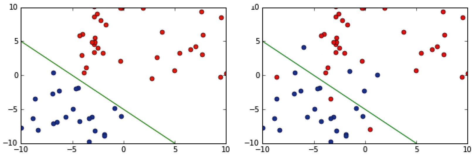
In the following diagram, at the top and bottom, we can see two classes of points (red and blue) that are in a two-dimensional feature space (the x and y axes). If both the x and y values of a point are below 5, then the point is blue. In all other cases, the point is red. In this case, the classes are linearly separable, meaning we can separate them with a hyperplane. Conversely, the classes in the image on the right are linearly inseparable:
Figure 1.2 – A linearly separable set of points (left) and a linearly inseparable set (right)
The SVM tries to find a hyperplane that maximizes the distance between itself and the points. In other words, from all possible hyperplanes that can separate the samples, the SVM finds the one that has the maximum distance from all points. In addition, SVMs can deal with data that is not linearly separable. There are two methods for this: introducing soft margins or using the kernel trick
Soft margins work by allowing a few misclassified elements while retaining the most predictive ability of the algorithm. In practice, it’s better not to overfit the ML model, and we could do so by relaxing some of the SVM hypotheses.
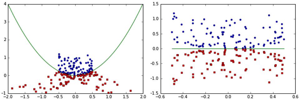
The kernel trick solves the same problem differently. Imagine that we have a two-dimensional feature space, but the classes are linearly inseparable. The kernel trick uses a kernel function that transforms the data by adding more dimensions to it. In our case, after the transformation, the data will be three-dimensional. The linearly inseparable classes in the two-dimensional space will become linearly separable in the three dimensions and our problem is solved:
Figure 1.3 – A non-linearly separable set before the kernel was applied (left) and the same dataset after the kernel has been applied, and the data can be linearly separated (right)
Lets move to the last one in our list, decision trees.
Decision trees
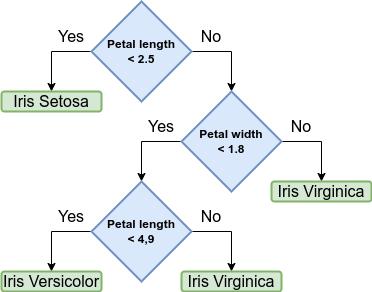
Another popular supervised algorithm is the decision tree, which creates a classifier in the form of a tree. It is composed of decision nodes, where tests on specific attributes are performed, and leaf nodes, which indicate the value of the target attribute. To classify a new sample, we start at the root of the tree and navigate down the nodes until we reach a leaf.
A classic application of this algorithm is the Iris flower dataset (http://archive.ics. uci.edu/ml/datasets/Iris), which contains data from 50 samples of three types of irises (Iris Setosa, Iris Virginica, and Iris Versicolor). Ronald Fisher, who created the dataset, measured four different features of these flowers:
• The length of their sepals
• The width of their sepals
• The length of their petals
• The width of their petals
Based on the different combinations of these features, it’s possible to create a decision tree to decide which species each flower belongs to. In the following diagram, we have defined a decision tree that will correctly classify almost all the flowers using only two of these features, the petal length and width:
1.4 – A decision tree for classifying the Iris dataset
To classify a new sample, we start at the root note of the tree (petal length). If the sample satisfies the condition, we go left to the leaf, representing the Iris Setosa class. If not, we go right to a new node (petal width). This process continues until we reach a leaf.
In recent years, decision trees have seen two major improvements. The first is random forests, which is an ensemble method that combines the predictions of multiple trees. The second is a class of algorithms called gradient boosting, which creates multiple sequential decision trees, where each tree tries to improve the errors made by the previous tree. Thanks to these improvements, decision trees have become very popular when working with certain types of data. For example, they are one of the most popular algorithms used in Kaggle competitions.
Unsupervised learning
The second class of ML algorithms is unsupervised learning. Here, we don’t label the data beforehand; instead, we let the algorithm come to its conclusion. One of the advantages of unsupervised learning algorithms over supervised ones is that we don’t need labeled data. Producing labels for supervised algorithms can be costly and slow. One way to solve this issue is to modify the supervised algorithm so that it uses less labeled data; there are different techniques for this. But another approach is to use an algorithm, which doesn’t need labels in the first place. In this section, we’ll discuss some of these unsupervised algorithms.
Clustering
One of the most common, and perhaps simplest, examples of unsupervised learning is clustering. This is a technique that attempts to separate the data into subsets.
Figure
To illustrate this, let’s view the spam-or-not-spam email classification as an unsupervised learning problem. In the supervised case, for each email, we had a set of features and a label (spam or not spam). Here, we’ll use the same set of features, but the emails will not be labeled. Instead, we’ll ask the algorithm, when given the set of features, to put each sample in one of two separate groups (or clusters). Then, the algorithm will try to combine the samples in such a way that the intraclass similarity (which is the similarity between samples in the same cluster) is high and the similarity between different clusters is low. Different clustering algorithms use different metrics to measure similarity. For some more advanced algorithms, you don’t have to specify the number of clusters.
The following graph shows how a set of points can be classified to form three subsets:
1.5 – Clustering a set of points in three subsets
K-means
K-means is a clustering algorithm that groups the elements of a dataset into k distinct clusters (hence the k in the name). Here’s how it works:
1. Choose k random points, called centroids, from the feature space, which will represent the center of each of the k clusters.
2. Assign each sample of the dataset (that is, each point in the feature space) to the cluster with the closest centroid.
3. For each cluster, we recomputed new centroids by taking the mean values of all the points in the cluster.
4. With the new centroids, we repeat Steps 2 and 3 until the stopping criteria are met.
The preceding method is sensitive to the initial choice of random centroids, and it may be a good idea to repeat it with different initial choices. It’s also possible for some centroids to not be close to any of
Figure
the points in the dataset, reducing the number of clusters down from k. Finally, it’s worth mentioning that if we used k-means with k=3 on the Iris dataset, we may get different distributions of the samples compared to the distribution of the decision tree that we’d introduced. Once more, this highlights how important it is to carefully choose and use the correct ML method for each problem.
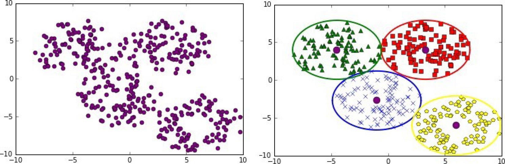
Now, let’s discuss a practical example that uses k-means clustering. Let’s say a pizza delivery place wants to open four new franchises in a city, and they need to choose the locations for the sites. We can solve this problem with k-means:
1. Find the locations where pizza is ordered most often; these will be our data points.
2. Choose four random points where the sites will be located.
3. By using k-means clustering, we can identify the four best locations that minimize the distance to each delivery place:
Figure 1.6 – The distribution of points where pizza is delivered most often (left); the round points indicate where the new franchises should be located and their corresponding delivery areas (right)
Self-supervised learning
Self-supervised learning refers to a combination of problems and datasets, which allow us to automatically generate (that is, without human intervention) labeled data from the dataset. Once we have these labels, we can train a supervised algorithm to solve our task. To understand this concept better, let’s discuss some use cases:
• Time series forecasting: Imagine that we have to predict the future value of a time series based on its most recent historical values. Examples of this include stock (and nowadays crypto) price prediction and weather forecasting. To generate a labeled data sample, let’s take a window with length k of the historical data that ends at past moment t. We’ll take the historical values in the range [t – k; t] and we’ll use them as input for the supervised algorithm. We’ll also take the historical value at moment t + 1 and we’ll use it as the label for the given input sample. We can apply this division to the rest of the historical values and generate a labeled training dataset automatically.