Published by John Wiley & Sons, Inc., Hoboken, New Jersey
Published simultaneously in Canada
No part of this publication may be reproduced, stored in a retrieval system, or transmitted in any form or by any means, electronic, mechanical, photocopying, recording, scanning, or otherwise, except as permitted under Section 107 or 108 of the 1976 United States Copyright Act, without either the prior written permission of the Publisher, or authorization through payment of the appropriate per-copy fee to the Copyright Clearance Center, Inc , 222 Rosewood Drive, Danvers, MA 01923, (978) 750-8400, fax (978) 750-4470, or on the web at www copyright com Requests to the Publisher for permission should be addressed to the Permissions Department, John Wiley & Sons, Inc., 111 River Street, Hoboken, NJ 07030, (201) 748-6011, fax (201) 748-6008, or online at http://www wiley com/go/permissions
Limit of Liability/Disclaimer of Warranty: While the publisher and author have used their best efforts in preparing this book, they make no representations or warranties with respect to the accuracy or completeness of the contents of this book and specifically disclaim any implied warranties of merchantability or fitness for a particular purpose No warranty may be created or extended by sales representatives or written sales materials The advice and strategies contained herein may not be suitable for your situation You should consult with a professional where appropriate Neither the publisher nor author shall be liable for any loss of profit or any other commercial damages, including but not limited to special, incidental, consequential, or other damages
For general information on our other products and services or for technical support, please contact our Customer Care Department within the United States at (800) 762-2974, outside the United States at (317) 572-3993 or fax (317) 5724002
Wiley also publishes its books in a variety of electronic formats. Some content that appears in print may not be available in electronic formats For more information about Wiley products, visit our web site at www wiley com
Library of Congress Cataloging-in-Publication Data:
Baker, Kenneth R., 1943–Optimization modeling with spreadsheets / Kenneth R Baker – Third Edition
pages cm
Includes bibliographical references and index
ISBN 978-1-118-93769-3 (hardback)
1 Mathematical optimization 2 Managerial economics–Mathematical models 3 Electronic spreadsheets 4 Programming (Mathematics) I Title
HB143.7.B35 2015 005 54–dc23 2015011069
Cover image courtesy of Kenneth R Baker
PREFACE
This is an introductory textbook on optimization that is, on mathematical programming intended for undergraduates and graduate students in management or in engineering The principal coverage includes linear programming, nonlinear programming, integer programming, and heuristic programming; and the emphasis is on model building using Microsoft® Office Excel® and Solver
The emphasis on model building (rather than algorithms) is one of the features that make this book distinctive. Most textbooks devote more space to algorithmic details than to formulation principles. These days, however, it is not necessary to know a great deal about algorithms in order to apply optimization tools, especially when relying on the spreadsheet as a solution platform.
The emphasis on spreadsheets is another feature that makes this book distinctive. Few textbooks devoted to optimization pay much attention to spreadsheet implementation of optimization principles, and many books that emphasize model building ignore spreadsheets entirely Thus, someone looking for a spreadsheet-based treatment would otherwise have to use a textbook that was designed for some other purpose, such as a survey of management science topics, rather than one devoted to optimization.
WHYMODELBUILDING?
The model building emphasis derives from an attempt to be realistic about what management and engineering students need most when learning about optimization. At an introductory level, the most practical and motivating theme is the wide applicability of optimization tools To apply optimization effectively, the student needs more than a brief exposure to a series of numerical examples, which is the way that most mathematical programming books treat applications With a systematic modeling emphasis, the student can begin to see the basic structures that appear in optimization models and, as a result, develop an appreciation for potential applications well beyond the examples in the text.
Formulating optimization models is both an art and a science, and this book pays attention to both. The art can be refined with practice, especially supervised practice, just the way a student would learn sculpture or painting. The science is reflected in the structure that organizes the topics in this book. For example, there are several distinct problem types that lend themselves to linear programming formulations, and it makes sense to study these types systematically In that spirit, the book builds a library of templates against which new problems can be compared. Analogous structures are developed for the presentation of other topics as well
WHYSPREADSHEETS?
Now that optimization tools have been made available with spreadsheets (i.e., with Excel), every spreadsheet user is potentially a practitioner of optimization techniques No longer do practitioners of optimization constitute an elite, highly trained group of quantitative specialists who are well versed in computer software Now, anyone who builds a spreadsheet model can call on optimization techniques and can do so without any need to learn about specialized software. The basic optimization tool, in the form of Excel’s Standard Solver, is now as readily available as the spellchecker. So why not raise modeling ability up to the level of software access? Let’s not pretend that most users of optimization tools will be inclined to shop around for algebraic modeling languages and industrial-strength “solvers” if they want to produce numbers. More likely, they will be drawn to Excel.
Students using this book can take advantage of even more powerful software packages (Analytic Solver Platform and OpenSolver) by using the material in the online appendices For the instructor who wants students to be working on one of these platforms, the book provides sufficient information to get started and to learn the user interface
WHAT’SSPECIAL?
Mathematical programming techniques have been invented and applied for more than half a century, so by now they represent a relatively mature area of applied mathematics There is not much new that can be said in an introductory textbook regarding the underlying concepts. The innovations in this book can instead be found in the delivery and elaboration of certain topics, making them accessible and understandable to the novice. The most distinctive of these features are as follows:
The major topics are not illustrated merely with a series of numerical examples Instead, the chapters introduce a classification for the problem types. An early example is the organization of basic linear programming models in Chapter 2 along the lines of allocation, covering, and blending models. This classification strategy, which extends throughout the book, helps the student to see beyond the particular examples to the breadth of possible applications.
Network models are a special case of linear programming models. If they are singled out for special treatment at all in optimization books, they are defined by a strict requirement for mass balance. Here, in Chapter 3, network models are presented in a broader framework, which allows for a more general form of mass balance, thereby extending the reader’s capability for recognizing and analyzing network problems.
Interest has been growing in data envelopment analysis (DEA), a special kind of linear programming application. Although some books illustrate DEA with a single example, this book provides a systematic introduction to the topic by providing a patient, comprehensive treatment in Chapter 5.
Analysis of an optimization problem does not end when the computer displays the numbers in an optimal solution Finding a solution must be followed with a meaningful interpretation of the results, especially if the optimization model was built to serve a client. An important framework for interpreting linear programming solutions is the identification of patterns, which is discussed in detail in Chapter 4.
The topic of heuristic programming has developed somewhat outside the field of optimization. Although various specialized heuristic approaches have been developed, generic software has seldom been available. Now, however, the advent of the evolutionary solver brings heuristic programming alongside linear and nonlinear programming as a generic software tool for pursuing optimal decisions The evolutionary solver is covered in Chapter 9
Beyond these specific innovations, as this book goes to print, there is no optimization textbook exclusively devoted to model building rather than algorithms that relies on the spreadsheet platform The reliance on spreadsheets and on a model building emphasis is the most effective way to bring optimization capability to the many users of Excel.
WHAT’SNEW?
The Third Edition largely follows the topic coverage of the previous edition, with one important change. In the new edition, the presentation is organized around the use of Excel’s Solver. More advanced software, such as Analytic Solver Platform or OpenSolver, might be preferred by some instructors, so the Third Edition provides support for both of these in online appendices. However, students need access to no software other than Excel in order to follow the coverage in the book’s nine chapters
The set of homework exercises has been expanded in the Third Edition Each chapter now contains about ten homework exercises, most of which appeared in the previous edition. In addition, a supplementary set of homework exercises can be found online for instructors who are looking for a broader set of exercises or for students who want additional practice.
THEAUDIENCE
This book is aimed at management students and secondarily to engineering students In business curricula, a course focused on optimization is viable in two situations. If there is no required introduction to management science at all, then the treatment of management science at the elective level is probably best done with specialized courses on deterministic and probabilistic models. This book is an ideal text for a first course dedicated to deterministic models If instead there is a required introduction to management science, chances are that the coverage of optimization glides
by so quickly that even the motivated student is left wanting more detail, more concepts, and more practice This book is also well suited to a second-level course that delves specifically into mathematical programming applications.
In engineering curricula, it is still typical to find a full course on optimization, usually as the first course on (deterministic) modeling Even in this setting, though, traditional textbooks tend to leave it to the student to seek out spreadsheet approaches to the topic, while covering the theory and perhaps encouraging students to write code for algorithms This book can capture the energies of students by covering what they would be spending most of their time doing in the real world building and solving optimization problems on spreadsheets.
This book has been developed around the syllabi of two courses at Dartmouth College that have been delivered for several years One course is a second-year elective for MBA students who have had a brief, previous exposure to optimization during a required core course that surveyed other analytic topics A second course is a required course for engineering management students in a graduate program at the interface between business and engineering. These students have had no formal exposure to spreadsheet modeling, although some may previously have taken a survey course in operations research. Thus, the book has proven to be appropriate for students who are about to study optimization with only a brief or nonexistent exposure to the subject.
ACKNOWLEDGMENTS
As I wrote in the preface to the first edition, I can trace the roots of this book to my collaboration with Steve Powell. Using spreadsheets to teach optimization is part of a broader activity in which Steve has been an active and inspiring leader, and I continue to benefit from his colleagueship. Several people contributed to the review process with constructive feedback and suggestions. For their help in this respect, I want to acknowledge Tim Anderson (Portland State University), David T Bourgeois (Southern New Hampshire University), Jeffrey Camm (University of Cincinnati), Ivan G. Guardiola (Missouri University of Science & Technology), Rich Metters (Texas A&M University), Jamie Peter Monat (Worcester Polytechnic Institute), Khosrow Moshirvaziri (California State University, Long Beach), Susan A Slotnick (Cleveland State University), and Mohit Tawarmalani (Purdue University).
The Third Edition makes only minor changes in the coverage of the previous edition, the main exception being the reliance on Excel’s Solver To make this software emphasis possible, it was critical to have an updated package for sensitivity analysis, and this was accomplished in a timely and professional manner by Bob Burnham In addition, there were many details to manage in preparing a new manuscript, and I was helped by several people willing to pay attention to details in order to improve the final product. I particularly want to thank Bill MacKinnon, Alex Zunega, and Geneva Trotter for their efforts.
Once again, I offer sincere thanks to my current editor, Susanne Steitz-Filler, for her support in planning and realizing the publication of a new edition. With her help and guidance, I am hopeful that the pleasures of optimization modeling will be experienced by yet another generation of students.
INTRODUCTIONTOSPREADSHEETMODELSFOR OPTIMIZATION
This is a book about optimization with an emphasis on building models and using spreadsheets Each facet of this theme models, spreadsheets, and optimization has a role in defining the emphasis of our coverage.
A model is a simplified representation of a situation or problem. Models attempt to capture the essential features of a complicated situation so that it can be studied and understood more completely. In the worlds of business, engineering, and science, models aim to improve our understanding of practical situations Models can be built with tangible materials, or words, or mathematical symbols and expressions. A mathematical model is a model that is constructed and also analyzed using mathematics In this book, we focus on mathematical models Moreover, we work with decision models, or models that contain representations of decisions. The term also refers to models that support decision-making activities
A spreadsheet is a row-and-column layout of text, numerical data, and logical information. The spreadsheet version of a model contains the model’s elements, linked together by specific logical information. Electronic spreadsheets, like those built using Microsoft® Office Excel® , have become familiar tools in the business, engineering, and scientific worlds. Spreadsheets are relatively easy to understand, and people often rely on spreadsheets to communicate their analyses. In this book, we focus on the use of spreadsheets to represent and analyze mathematical models
This text is written for an audience that already has some familiarity with Excel. Our coverage assumes a level of facility with Excel comparable to a beginner’s level. Someone who has used other people’s spreadsheets and built simple spreadsheets for some purpose either personal or organizational has probably developed this skill level. Box 1.1 describes the Excel skill level assumed Readers without this level of background are encouraged to first work through some introductory materials, such as the books by McFedries (1) and Walkenbach (2).
BOX1.1ExcelSkillsAssumedasBackgroundforThisBook
Navigating in workbooks, worksheets, and windows
Using the cursor to select cells, rows, columns, and noncontiguous cell ranges
Entering text and data; copying and pasting; filling down or across
Formatting cells (number display, alignment, font, border, and protection)
Editing cells (using the formula bar and cell edit capability [F2])
Entering formulas and using the function wizard
Using relative and absolute addresses
Using range names
Creating charts and graphs
Optimization is the process of finding the best values of the variables for a particular criterion or, in our context, the best decisions for a particular measure of performance. The elements of an optimization problem are a set of decisions, a criterion, and perhaps a set of required conditions, or constraints, that the decisions must satisfy. These elements lend themselves to description in a mathematical model The term optimization sometimes refers specifically to a procedure that is implemented by software. However, in this book, we expand that perspective to include the modelbuilding process as well as the process of finding the best decisions
Not all mathematical models are optimization models. Some models merely describe the logical relationship between inputs and outputs Optimization models are a special kind of model in which the purpose is to find the best value of a particular output measure and the choices that produce it. Optimization problems abound in the real world, and if we ’ re at all ambitious or curious, we often find ourselves seeking solutions to those problems. Business firms are very interested in optimization because making good decisions helps a firm run efficiently, perform profitably, and compete effectively. In this book, we focus on optimization problems expressed in the form of spreadsheet models and solved using a spreadsheet-based approach.
1.1ELEMENTSOFAMODEL
To restate our premise, we are interested in mathematical models. Specifically, we are interested in two forms algebraic and spreadsheet models. In the former, we use algebraic notation to represent elements and relationships, and in the latter, we use spreadsheet entries and structure. For example, in an algebraic statement, we might use the variable x to represent a quantitative decision, and we might use some function f(x) to represent the measure of performance that results from choosing decision x. Then, we might adopt the letter z to represent a criterion for decision making and construct the equation z = f(x) to guide the choice of a decision Algebra is the basic language of analysis largely because it is precise and compact.
As an introductory modeling example, let’s consider the price decision in the scenario of Example 1 1
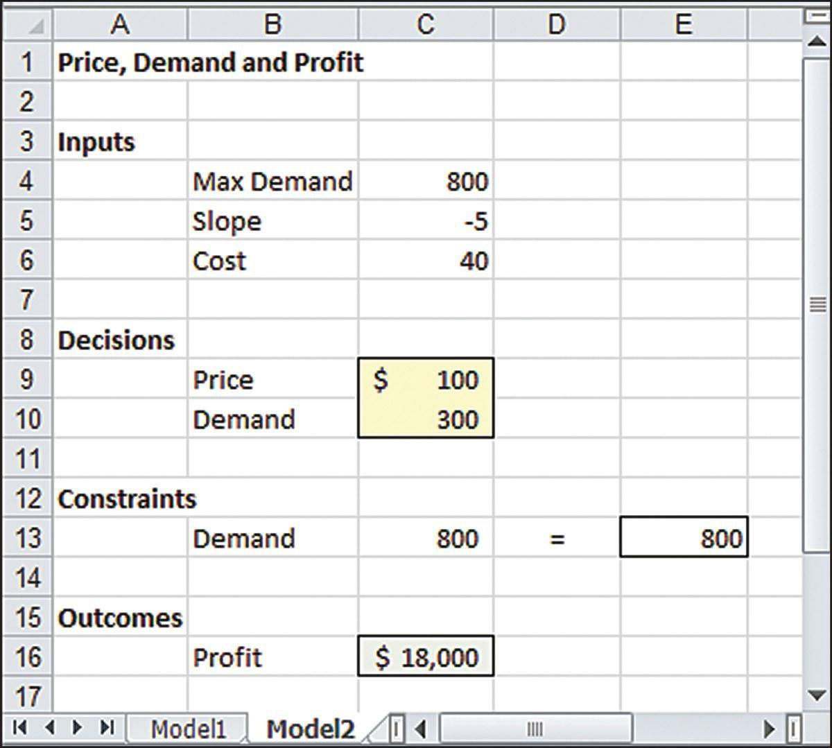
EXAMPLE1.1 Price,Demand,andProfit
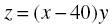
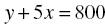
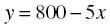
Our firm’s production department has carried out a cost accounting study and found that the unit cost for one of its main products is $40. Meanwhile, the marketing department has estimated the relationship between price and sales volume (the so-called demand curve for the product) as follows:
where y represents quarterly demand and x represents the selling price per unit. We wish to determine a selling price for this product, given the information available.
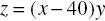
In Example 1.1, the decision is the unit price, and the consequence of that decision is the level of demand The demand curve in Equation 1 1 expresses the relationship of demand and price in algebraic terms. Another equation expresses the calculation of profit contribution, by multiplying the demand y by the unit profit contribution (x 40) on each item
where z represents our product’s quarterly profit contribution
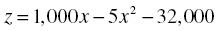
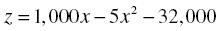
We can substitute Equation 1 1 into 1 2 if we want to write z algebraically as a function of x alone As a result, we can express the profit contribution as
This step embodies the algebraic principle that simplification is always desirable. Here, simplification reduces the number of variables in the expression for profit contribution. Simplification, however, is not necessarily a virtue when we use a spreadsheet model
Example 1.1 has some important features. First, our model contains three numerical inputs: 40 (the unit cost), 5 (the marginal effect of price on demand), and 800 (the maximum demand). Numerical inputs such as these are called parameters In some models, parameters correspond to raw data, but in many cases, parameters are summaries drawn from a more primitive data set. They may also be estimates made by a knowledgeable party, forecasts derived from statistical analyses, or predictions chosen to reflect a future scenario.
Our model also contains a decision an unknown quantity yet to be determined. In traditional
algebraic formulations, unknowns are represented as variables. Quantitative representations of decisions are therefore called decision variables The decision variable in our model is the unit price x.
Our model contains the equation that relates demand to price. We can think of this relationship as part of the model’s logic, prescribing a necessary relationship between two variables price and demand. Thus, in our model, the only admissible values of x and y are those that satisfy Equation 1 1
Finally, our model contains a calculation of quarterly profit contribution, which is the performance measure of interest and a quantity that we wish to maximize This output variable measures the consequence of selecting any particular price decision in the model. In optimization models, we are concerned with maximizing or minimizing some measure of performance, expressed as a mathematical function, and we refer to it as the objective function, or simply the objective.
1.2SPREADSHEETMODELS
Algebra is an established language that works well for describing problems, but not always for obtaining solutions. Algebraic solutions tend to occur in formulas, not numbers, but numbers most often represent decisions in the practical world By contrast, spreadsheets represent a practical language one that works very effectively with numbers. Like algebraic models, spreadsheets can be precise and compact, but there are also complications that are unique to spreadsheets For example, there is a difference between form and content in a spreadsheet. Two spreadsheets may look the same in terms of the numbers displayed on a computer screen, but the underlying formulas in corresponding cells could differ. Because the information behind the display can be different even when two spreadsheets have the same on-screen appearance, we can’t always determine the logical content from the form of the display Another complication is the lack of a single, well-accepted way to build a spreadsheet representation of a given model. In an optimization model, we want to represent decision variables, an objective function, and constraints However, that still leaves a lot of flexibility in choosing how to incorporate the logic of a particular model into a spreadsheet. Such flexibility would ordinarily be advantageous if the only use of a spreadsheet were to help individuals solve problems. But spreadsheets are perhaps even more important as vehicles for communication. When we use spreadsheets in that role, flexibility can sometimes lead to confusion and disrupt the intended communication.
We will try to mitigate these complications with some design guidelines. For example, it is helpful to create separate modules in the spreadsheet for decision variables, objective function, and constraints. To the extent that we follow such guidelines, we may lose some flexibility in building a spreadsheet model. Moving the design process toward standardization will, however, make the content of a spreadsheet more understandable from its form, so differences between form and content become less problematic.
With optimization, a spreadsheet model contains the analysis that ultimately provides decision support For this reason, the spreadsheet model should be intelligible to its users, not just to its developer. On some occasions, a spreadsheet might come into routine use in an organization, even when the developer moves on. New analysts may inherit the responsibilities associated with the model, so it is vital that they, too, understand how the spreadsheet works. For that matter, the decision maker may also move on. For the organization to retain the learning that has taken place, successive decision makers must also understand the spreadsheet In yet another scenario, the analyst develops a model for one-time use but then discovers a need to reuse it several months later in a different context In such a situation, it’s important that the analyst understands the original model, lest the passage of time obscure its purpose and logic. In all of these cases, the spreadsheet model fills a significant communications need Thus, it is important to keep the role of communication in mind while developing a spreadsheet.
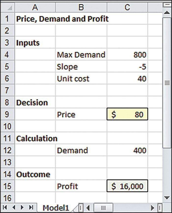
A spreadsheet version of our pricing model might look like the one in Figure 1.1. This spreadsheet contains a cell (C9) that holds the unit price, a cell (C12) that holds the level of demand, and a cell (C15) that holds the total profit contribution. Actually, cell C12 holds Equation 1.1 in the form of the Excel formula = C4 + C5 * C9 Similarly, cell C15 holds Equation 1 2 with the formula =(C9 C6) * C12. In cell C9, the unit price is initially set to $80. For this choice, demand is 400, and the quarterly profit contribution is $16,000.
Figure 1.1 Spreadsheet model for determining price
In a spreadsheet model, there is usually no premium on being concise, as there is when we use algebra. In fact, when conciseness begins to interfere with a model’s transparency, it becomes undesirable. Thus, in Figure 1.1, the model retains the demand equation and displays the demand quantity explicitly; we have not tried to incorporate Equation 1.3. This form allows a user to see how price influences profit contribution through demand because all of these quantities are explicit Furthermore, it is straightforward to trace the connection between the three input parameters and the calculation of profit contribution
To summarize, our model consists of three parameters and a decision variable, together with some intermediate calculations, all leading to an objective function that we want to maximize. In algebraic terms, the model consists of Equations 1 1 and 1 2, with the prescription that we want to maximize Equation 1.2. In spreadsheet terms, the model consists of the spreadsheet in Figure 1.1, with the prescription that we want to maximize the value in cell C15
The spreadsheet is organized into four modules: inputs, decision, calculation, and outcome, separating different kinds of information In spreadsheet models, it is a good idea to separate input data from decisions and decisions from outcome measures. Intermediate calculations that do not lead directly to the outcome measure should also be kept separate
In the spreadsheet model, cell borders and shading draw attention to the decision (cell C9) and the objective (cell C15) as the two most important elements of the optimization model. No matter how complicated a spreadsheet model may become, we want the decisions and the objective to be located easily by someone who looks at the display.
In the spreadsheet of Figure 1 1, the input parameters appear explicitly It would not be difficult to skip the Inputs section entirely and express the demand function in cell C12 with the formula =800 5 * C9 or to express the profit contribution in cell C15 with the formula =(C9 40) * C12 This approach, however, places the numerical parameters in formulas, so a user would not see them at all when looking at the spreadsheet Good practice calls for displaying parameters explicitly in the spreadsheet, as we have done in Figure 1.1, rather than burying them in formulas.
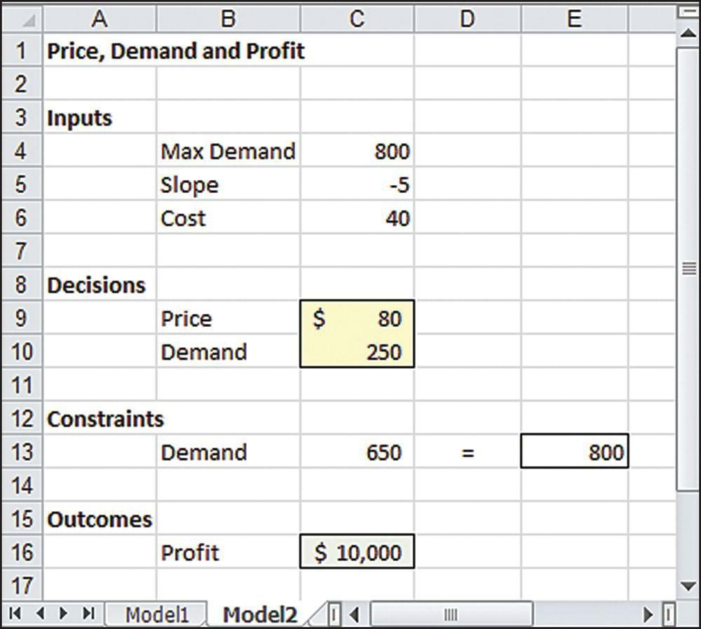
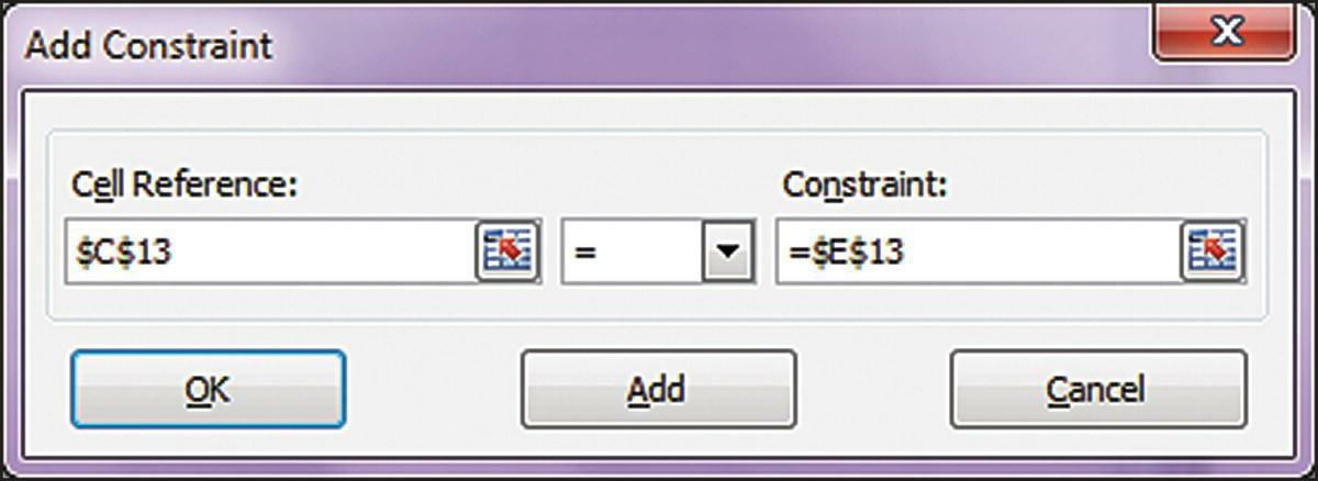
The basic version of our model, shown in Figure 1.1, is ready for optimization. But let’s look at an alternative, shown in Figure 1 2 This version contains the four modules, and the numerical inputs are explicit but placed differently than in Figure 1.1. The main difference is that demand is treated as a decision variable and the demand curve is expressed as an explicit constraint. Specifically, this form of the model treats both price and demand as variables in cells C9:C10, as if the two choices could be made arbitrarily. However, the constraints module describes a relationship between the two variables in the form of Equation 1 1, which can equivalently be expressed as
(1.4)
Figure 1.2 Alternative spreadsheet model for determining price.
We can meet this constraint by forcing cell C13 to equal cell E13, a condition that does not yet hold in Figure 1.2. Cell C13 contains the formula on the left-hand side of Equation 1.4, and cell E13 contains a reference to the parameter 800 The equals sign between them, in cell D13, signifies the nature of the constraint relationship to someone who is looking at the spreadsheet and trying to understand its logic Equation 1 4 collects all the terms involving decision variables on the left-hand side (in cell C13) and places the constant term on the right-hand side (in cell E13). This is a standard form for expressing a constraint in a spreadsheet model The spreadsheet itself displays, but does not actually enforce, this constraint. The enforcement task is left to the optimization software. Once the constraint is met, the corresponding decisions are called feasible
This is a good place to include a reminder about the software that accompanies this book. The software contains important files and programs In terms of files, the book’s website1 contains all of the spreadsheets shown in the figures. Figures 1.1 and 1.2, for example, can be found in the file that contains the spreadsheets for Chapter 1 Those files should be loaded, or else built from scratch, before continuing with the text. As we proceed through the chapters, the reader is welcome to load each file that appears in a figure, for hands-on examination
1.3AHIERARCHYFORANALYSIS
Before we proceed, some background on the development of models in organizations may be useful. Think about the person who builds a model as an analyst, someone who provides support to a decision maker or client. (In some cases, the analyst and the client are the same.) The development, testing, and application of a model constitute support for the decision maker a service to the client The application phase of this process includes some standard stages of model use.
When a model is built as an aid to decision making, the first stage often involves building a prototype, or a series of prototypes, leading to a model that the analyst and the client accept as a usable decision-support tool. That model provides quantitative analysis of a base-case scenario. In Example 1 1, suppose we set a tentative unit price of $80 This price might be called a base case, in the sense that it represents a tentative decision. As we have seen, this price leads to demand of 400 and profit contribution of $16,000.
After establishing a base case, it is usually appropriate to investigate the answers to a number of “what-if” questions We ask, what if we change a numerical input or a decision in the model what impact would that change have? Suppose, for example, that the marginal effect of price on demand (the slope of the demand curve) were 4 instead of 5 What difference would this make? Retracing our algebraic steps, or revising the spreadsheet in Figure 1.1, we can determine that the profit contribution would be $19,200.
Systematic investigations of this kind are called sensitivity analyses They explore how sensitive the results and conclusions are to changes in assumptions. Typically, we start by varying one assumption at a time and tracing the impact. Then, we might try varying two or more assumptions, but such probing can quickly become difficult to follow Therefore, most sensitivity analyses are performed one assumption at a time. Sometimes, it is useful to explore the what-if question in reverse That is, we might ask, for the result to attain a given outcome level, what would the numerical input have to be? For example, starting with the base-case model, we might ask, what unit price would generate a profit contribution of $17,000? We can answer this question algebraically, by setting z = 17,000 in Equation 1.3 and solving for x, or, with the spreadsheet model, we can invoke Excel’s Goal Seek tool to discover that the price would have to be about $86 (Actually, this is one of two prices that would deliver a profit contribution of $17,000.)
Sensitivity analyses are helpful in determining the robustness of the results and any risks that might be present. They can also reveal how to achieve improvement from better choices in decision making However, locating improvements this way is something of a trial-and-error process, which is inefficient. Faster and more reliable ways of locating improvements are available. Moreover, with trial-and-error approaches, we seldom know how far improvements can potentially reach, so a best outcome could exist that we never detect.
From this perspective, optimization can be viewed as a sophisticated form of sensitivity analysis that seeks the best values for the decisions and the best value for the performance measure Optimization takes us beyond mere improvement; we look for the very best outcome in our model, the maximum possible benefit or the minimum possible cost If we have constraints in our model, then
optimization also tells us which of those conditions ultimately limit what we want to accomplish. Optimization can also reveal what we might gain if we can find a way to overcome those constraints and proceed beyond the limitations they impose.
1.4OPTIMIZATIONSOFTWARE
Optimization procedures find the best values of the decision variables in a given model In the case of Excel, the optimization software is known as Solver, which is a standard tool available on the Data ribbon (The generic term solver often refers to optimization software, whether or not it is implemented in a spreadsheet.) Optimization tools have been available on computers for several decades and predate the widespread use of electronic spreadsheets Before spreadsheets became popular, optimization was available as stand-alone software. It relied on an algebraic approach and was often accessible only by technical experts. Decision makers and even their analysts had to rely on those experts to build and solve optimization models. Spreadsheets, if they were used at all, were limited to small examples. Now, however, the spreadsheet allows decision makers to develop their own models, without having to learn specialized software, and to find optimal solutions for those models using Solver. Two trends account for the popularity of spreadsheet optimization. First, familiarity with spreadsheets has become almost ubiquitous, at least in the business world The spreadsheet has come to represent a common language for analysis. Second, the software packages available for spreadsheet-based optimization now include some of the most powerful tools available The spreadsheet platform need not be an impediment to solving practical optimization problems. Spreadsheet-based optimization has several advantages. The spreadsheet allows model inputs to be documented clearly and systematically Moreover, if it is necessary to convert raw data into other forms for the purposes of setting up a model, the required calculations can be performed and documented conveniently in the same spreadsheet, or at least on another sheet in the same workbook. This allows integration between raw data and model data. Without this integration, errors or omissions are more likely, and maintenance becomes more difficult. Another advantage is algorithmic flexibility: The spreadsheet has the ability to call on several different optimization procedures, but the process of preparing the model is mostly the same no matter which procedure is applied Finally, spreadsheet models have a certain amount of intrinsic credibility because spreadsheets are now so widely used for other purposes. Although spreadsheets can contain errors (and often do), there is at least some comfort in knowing that logic and discipline must be applied in the building of a spreadsheet.
Table 1.1 summarizes and compares the advantages of spreadsheet and algebraic software approaches to optimization problems. The main advantage of algebraic approaches is the efficiency with which models can be specified With spreadsheets, the elements of a model are represented explicitly. Thus, if the model requires a hundred variables, then the model builder must designate a hundred cells to hold their respective values Algebraic codes use a different method If a model contains a hundred variables, the code might refer to x(k), with a specification that k may take on values from 1 to 100, but x(k) need not be represented explicitly for each of the hundred values
Table 1.1 Advantages of Spreadsheet and Algebraic Solution Approaches
Spreadsheet Approaches
Several algorithms available in one place
Integration of raw data and model data
Flexibility in layout and design
Ease of communication with nonspecialists
Intrinsic credibility
Algebraic Approaches
Large problem sizes accommodated
Concise model specification
Standardized model description
Enhancements possible for special cases
A second advantage of algebraic approaches is the fact that they can sometimes be tailored to a particular application. For example, the very large crew-scheduling applications used by airlines exhibit a special structure To exploit this structure in the solution procedure, algebraic codes are sometimes enhanced with specialized subroutines that add solution efficiencies when solving a crew-scheduling problem.
A disadvantage of using spreadsheets is that they are not always transparent. As noted earlier, the analyst has a lot of flexibility in the layout and organization of a spreadsheet, but this flexibility, taken too far, may detract from effective communication. In this book, we try to promote better
communication by suggesting standard forms for particular types of models By using some standardization, we make it easier to understand and debug someone else’s model Algebraic codes usually have very detailed specifications for model format, so once we ’ re familiar with the specifications, we should be able to read and understand anyone else’s model
In brief, commercially available algebraic solvers represent an alternative to spreadsheet-based optimization. In this book, our focus on a spreadsheet approach allows the novice to learn basic concepts of mathematical programming, practice building optimization models, obtain solutions readily, and interpret and apply the results of the analysis. All these skills can be developed in the accessible world of spreadsheets. Moreover, these skills provide a solid foundation for using algebraic solvers at some later date, when and if the situation demands it.
1.5USINGSOLVER
Excel’s Solver is an add-in that comes with Excel. An icon for Solver typically appears in the Data ribbon in the Analysis group. If the icon is not visible, it is possible to activate Solver by following the steps given below.
On the File tab, select Options and then Add-ins.
At the bottom of the window, set the drop-down menu to Manage Excel Add-ins. Then click Go
In the Add-ins window, check the box for Solver Add-in and click OK.
Purchasers of this book have the option to download a Windows-based software package called Analytic Solver Platform for Education (ASPE). ASPE was developed by the same team that created Excel’s Solver, and it will accommodate all models built with Excel’s Solver. However, ASPE is a more powerful version of Excel’s Solver and relies on a different user interface More information on ASPE can be found in Appendix 1.
In order to illustrate the use of Solver, we return to Example 1.1. The optimization problem is to find a unit price that maximizes quarterly profit contribution An algebraic statement of the problem is as follows:
This form of the model corresponds to Figure 1.2, which contains two decision variables (x and y, or price and demand) and one constraint on the decision variables The spreadsheet model in Figure 1.2 is ready for optimization.
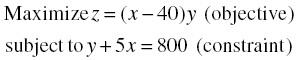
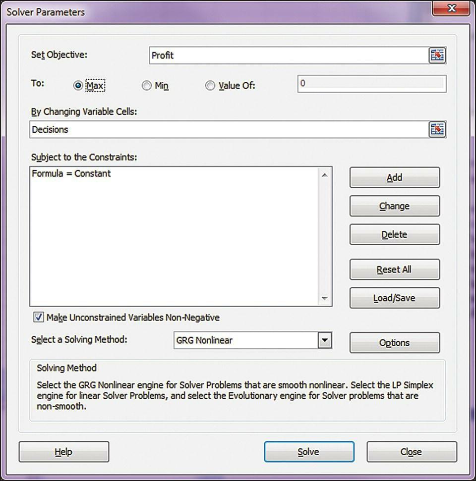
To start, we click on the Solver icon in the Data ribbon. This step opens the Solver Parameters window, shown in Figure 1.3. (The location of the cursor is reflected in the first data-entry window.) The Solver Parameters window allows us to specify our model in a way that’s consistent with the following sentence:
Figure 1.3 Solver Parameters window
Set objective C16 to a max[imum] by changing variable cells C9:C10 subject to the constraint C13 = E13
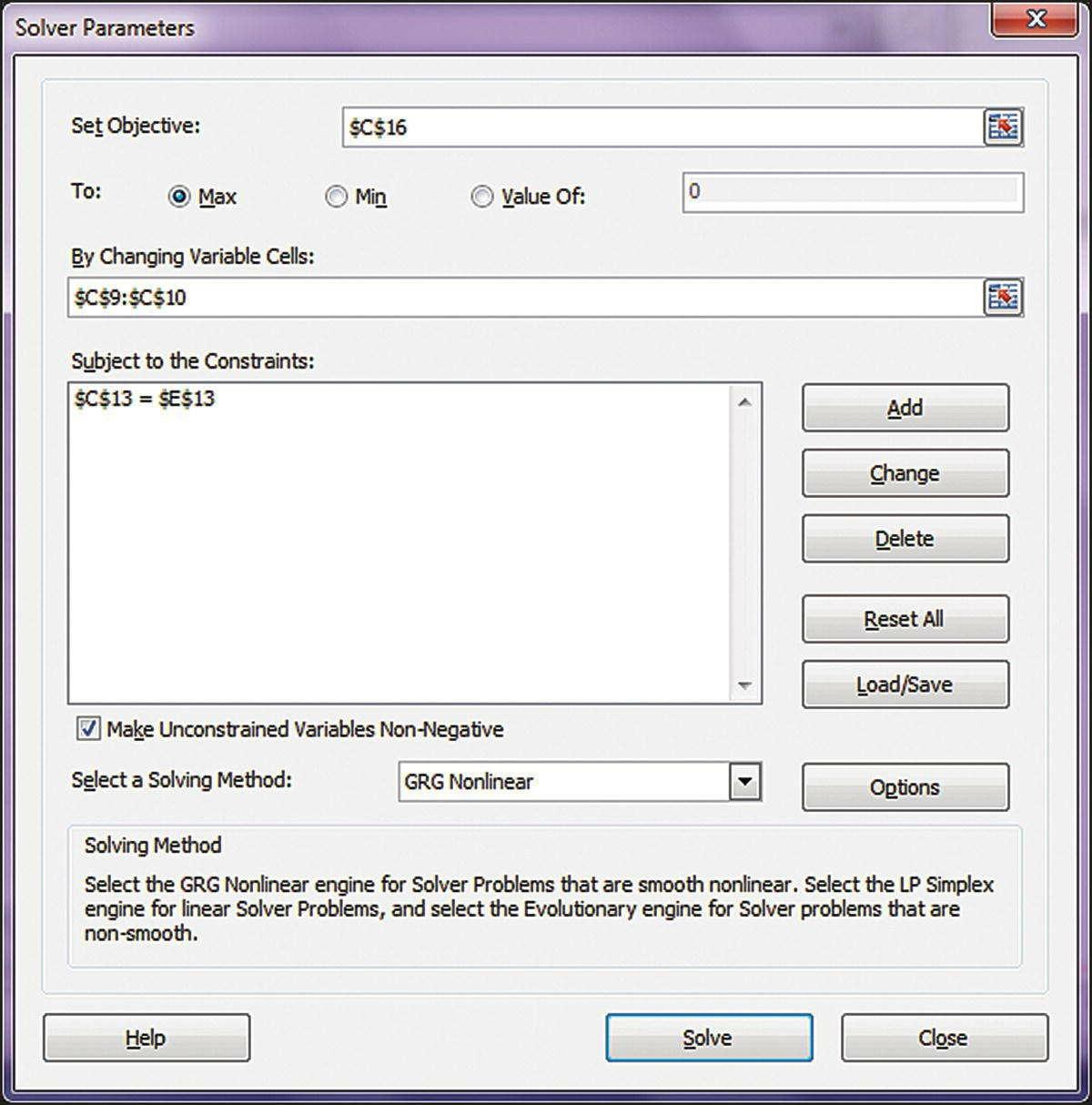
Three data-entry windows in Figure 1 3 allow us to make the specification In the Set Objective window, we point to C16 or enter C16, the address of the objective function; and on the next line, we select the button for Max (or confirm that it is already selected as the default) In the Changing Variable Cells window, we point to the two-cell range C9:C10. Then, to specify the constraint, we click the Add button, which opens the Add Constraint window Figure 1 4 shows this window as it looks when properly filled out, with the drop-down menu in the center to specify that the constraint is an equation
Figure 1.4 Add Constraint window.
In nearly all of the models we will encounter, negative values of the decision variables make no practical sense, so we typically want to require variables to be nonnegative The simplest way to impose this requirement is to check the box for making unconstrained variables nonnegative. (The reference to “unconstrained” variables allows us to impose more stringent constraints if we wish In our example, we might require the unit price to be at least 40 to ensure that profits will not be negative With such a constraint elsewhere in the model, it would be unnecessary to impose a nonnegative requirement on cell C9.)
When specifying constraints, one of our design guidelines for Solver models is to reference a cell containing a formula in the Cell Reference box and to reference a cell containing a number in the Constraint box. The use of cell references keeps the key parameters visible on the spreadsheet, rather than in the less accessible windows of Solver’s interface The principle at work here is to communicate as much as possible about the model using the spreadsheet itself. Ideally, another person would not have to examine the Solver Parameters window to understand the model. (Although Solver permits us to enter numerical values directly into the Constraint box, this form is less effective for communication and complicates sensitivity analysis. It would be reasonable only in special cases where the model structure is obvious from the spreadsheet and where we expect to perform no sensitivity analyses for the corresponding parameter.)
Finally, we specify a solving method for the optimization. In this case, the default choice (GRG Nonlinear) is appropriate, so nothing else is needed The specification is complete, and pressing Solve invokes the optimization procedure. (Alternatively, pressing Close saves the specification on the spreadsheet but does not run the optimization procedure.)
In summary, our model specification is the following:
Objective:C16 (maximize)
Variables:C9:C10
Constraint: C13 = E13
When we invoke the GRG Nonlinear procedure, Solver searches for the optimal price and ultimately places it in cell C9, as shown in Figure 1 5
1.5 Optimal solution produced by Solver
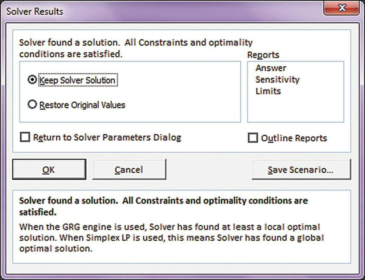
The result of the optimization run is summarized in the Solver Results window, shown in Figure 1.6, which opens when the optimization run completes. The message at the top of the window states, “Solver found a solution All Constraints and optimality conditions are satisfied ” This optimality message, which is elaborated at the bottom of the window, tells us that no problems arose during the optimization and Solver was able to find an optimal solution The profit-maximizing unit price is $100, yielding an optimal profit of $18,000. No other price can achieve more than this level. Thus, if we are confident that the demand curve continues to hold, the profit-maximizing decision would be to set the unit price at $100.
Figure
Figure 1.6 Solver Results window
Finally, the Solver Results window allows us to select a button to preserve the solution on the spreadsheet (as in Fig. 1.5) or to restore the values that were in the spreadsheet before the optimization run
We have used Example 1 1 to introduce Solver and its user interface This interface offers us several options that are not a concern in this problem. In later chapters, we cover many of these settings and discuss when they become relevant We also discuss the variations that can occur in optimization runs. For example, depending on the initial values of the decision variables, the nonlinear solver may generate the following message: “Solver has converged to the current solution All constraints are satisfied.” This convergence message indicates that Solver has not been able to confirm optimality Usually, this condition occurs because of numerical issues in the solution algorithm, and the resolution is to rerun Solver from the point where convergence occurred. Normally, one or two iterations are sufficient to produce the optimality message. We discuss Solver’s result messages in more detail later.
Using Solver, we can minimize an objective function instead of maximizing it We simply select the button for Min rather than Max. (A third option allows us to specify a target value and find a set of variables that achieves the target value This is not an optimization tool, and we will not pursue this particular capability.)
When an optimization model contains several decision variables, we can enter them one at a time, separated by commas More conveniently, we can arrange the spreadsheet so that all the variables appear in adjacent cells, as in Figure 1.2, and reference their cell range with just one entry in the Solver Parameters window. Because most optimization problems have several decision variables, we save time by placing them in adjacent cells. This layout also makes the information in the Solver Parameters window easier to interpret when someone else is trying to audit our work or if we are reviewing it after not having seen it for a long time However, exceptions to this design guideline sometimes occur. Certain applications sometimes lead us to use nonadjacent locations for convenience in laying out the decision variable cells (Box 1 2)
BOX1.2ExcelMini-Lesson:UsingRangeNameswithSolver
Excel offers the opportunity to refer to a cell range using a custom name. The range name can be entered in the Name box (located just above the heading for column A) after selecting the desired range of cells. A one-cell range can be named in the same manner.
To show the effect of named ranges, we return to the model of Figure 1.2 and name the following cells:
Cells Name
C9:C10 Decisions
C13 Formula
E13 Constant
C16 Profit
Then, the Solver Parameters window describes the model with range names instead of cell references, as shown in Figure 1.7. When a new user examines the model, this form is likely to be more meaningful than the use of literal cell references because the range names provide both description and documentation. Thus, range names are valuable for situations in which communicating the model to other audiences is an important consideration. When Solver is applied in an organizational setting, the use of range names is normally desirable In the remainder of this book, however, we will continue to rely on cell references because they relate the information in the Solver Parameters window directly to the contents of the spreadsheet display.
Figure 1.7 Solver Parameters window for the model with range names.
SUMMARY
Many types of applications invite the use of Excel’s Solver. In one sense, then, this book is about using Solver to obtain solutions to optimization problems Because Solver is a spreadsheet tool, the book builds skill and confidence in applying spreadsheet-based methods. In another sense, this book is about the problem types that Solver can handle, but the information on how to run Solver is incidental. The transcendent theme is the building of optimization models. If Solver weren’t around to produce solutions, then some other software would perform the computational task. The more basic skill is creating the model in the first place and recognizing its potential role in decision support Because a variety of problem types is covered, this book provides insight into the kinds of applications that can be addressed with optimization techniques. Thus far, we have introduced six design guidelines for spreadsheet optimization models:
1. Separate inputs from decisions and decisions from outputs.
2. Create distinct modules for decision variables, objective function, and constraints.
3 Display parameters explicitly on the spreadsheet, rather than in formulas
4. Enter parameters in the spreadsheet, rather than in the Add Constraints window.
5. Place decision variables in adjacent cells.
6. Highlight important cells, such as the decision variables and the objective.
Subsequent chapters introduce additional features of good spreadsheet design. This is not a claim that each example spreadsheet is the only possible way of designing a model, or even that it’s the best way. A model should be easy to recognize, debug, use routinely, and pass on to others. A key feature of a good spreadsheet model is its ability to communicate clearly.
Solver does not consist of a single procedure. Solver actually consists of four main optimization procedures, which are covered in subsequent chapters We refer to these procedures as:
The nonlinear solver
The linear solver
The integer solver
The evolutionary solver
Chapters 2–5 deal with the linear solver, introducing many features of optimization analysis in the process Chapters 6 and 7 deal with models that can be solved with the integer solver, and Chapter 8 deals with the nonlinear solver. The evolutionary solver, which is introduced in Chapter 9, is not properly an optimization procedure in the same sense as the others, but it applies in situations where the other solvers might fail. Each chapter is filled with illustrative examples and followed by a set of practice exercises If readers work through the examples and the exercises, they will develop a firm grasp on how to solve practical optimization problems using spreadsheets.
EXERCISES
1.1 Determining an Optimal Price: A firm’s marketing department has estimated the demand curve of a product as y = 1100 7x, where y represents demand and x represents the unit selling price (in dollars) for the relevant decision period The unit cost is known to be $24 What price maximizes net income from sales of the product?
1.2 Pricing in Two Markets: Global Products, Inc has been making an electronic appliance for the domestic market. Demand for the appliance is price sensitive, and the demand curve is known to follow the linear function D = 4000 5P, where D represents annual demand and P represents selling price in the home currency, which is the frank (F). The cost of manufacturing the appliance is 100 F
For the coming year, Global is planning to sell the same product in a foreign market, where the currency is the marc (M). From surveys, the demand curve in the foreign country is estimated to follow a different linear function, D = 2000 2P, where the price is denominated in marcs
All production will be carried out at Global’s domestic plant, with the expectation that the unit cost will remain unchanged The exchange rate is 1 5 M/F, and Global plans to offer an equivalent price in both markets.
a. If Global were to operate exclusively in its domestic market, what would be its profitmaximizing price and its annual profit?
b. When Global sells in both markets at one equivalent price, what is its profit-maximizing price and its annual profit?
1.3 Locating a Distribution Center: Northeast Parts Supply is a wholesale distributor of components for printers, fax machines, scanners, and related equipment. Northeast stocks expensive spare parts, which dealers prefer not to hold, and offers same-day delivery on any order. The firm now serves eight dealers in the New England area and wishes to locate its distribution facility at a central point In particular, its dealers have each been assigned a location on an x y grid, and Northeast would like to find the best location for the distribution facility
The eight dealers and their grid locations are shown in the following table:
y-location 32 36 71 58 68 163 149 192
a. Determine the location that minimizes the sum of the distances from the distribution facility to the dealers
b Determine the location that minimizes the maximum distance from the distribution facility to any of the dealers.
1.4 Siting a Warehouse: An appliance dealer offers free delivery in any one of its five Texas cities, which will be serviced by a single warehouse. The distance from the warehouse site to a given city is considered to be a good proxy for the annual cost of providing delivery service, and the objective is to minimize the total distance from the warehouse to the five cities. The cities are treated as if they were each a single point located at a specific latitude and longitude, as listed in the table below. City Austin Houston Midland Tyler Waco
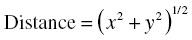
When locations are specified in terms of latitude (Lat) and longitude (Lon), a good approximation for the distance (in miles) between two locations is the following:
where x = 69 1 (Lat2 Lat1) and y = 69 1 (Lon2 Lon1) [cos(Lat1/57 3)]
What is the best location (latitude and longitude) for the warehouse?
1.5 Finding a Lost Plane: A private plane went down off the coast and sank during a bad storm although rescuers were able to save its crew Aboard the plane was a transmitter that was able to send out a signal for 72 hours after the plane went down. When the weather cleared, searchers went out in three different boats carrying equipment that could detect the signal and estimate its distance from the transmitter. The locations of the three boats on an x y grid and their distance estimates (in miles) are shown in the table below Searcher 1 2 3
x-location 25 35 70
y-location 60 40 10
Estimate 29 3 34 7 15 5
The estimates are known to be unreliable, but the information may sufficient to locate the sunken plane, at least approximately. What is its x y-location?
1.6 Collecting Credit Card Debt: A bank offers a credit card that can be used in various locations. The bank’s analysts believe that the percentage P of accounts receivable collected by t months after credit is issued increases at a decreasing rate Historical data suggest the following function:
The average credit issued in any 1 month is $125 million, and historical experience suggests that for new credit issued in any month, collection efforts cost $1 million/month
a Determine the number of months that collection efforts should be continued if the objective is to maximize the net collections (dollars collected minus collection costs). Allow for fractional months
b. Under the optimal policy in (a), what percentage of accounts receivable should be collected?
1.7 Allocating Plant Output: A firm owns five manufacturing plants that are responsible for the quarterly production of 50,000 pounds of an industrial solvent. The production process exhibits diseconomies of scale. At plant p, the cost of making x thousand pounds of the solvent is approximated by the quadratic function f(x) = (1/cp)x2 . The parameters cp are plant dependent, as shown in the following table.
p 1 2 3 4 5
How should production be allocated among the five plants in order to minimize the total cost of meeting the volume requirement?
1.8 Determining Production Lot Sizes: Four products are routed through a machining center that is notorious for its delays Each product has had stable demand for some time, so that average weekly demand is predictable over a 3–6 months’ time frame. However, in the short run, demand fluctuates a great deal, and the load at the machining center varies considerably. The production control system dictates the lot size for each of the products. These quantities are shown, along with other relevant information, in the following table.
With the current lot sizes, the machining center is running at a utilization of about 76%, but long lead times, sometimes over 2 weeks, have discouraged production planners from increasing its load (A week contains 120 productive hours ) In the past, lead times spiraled out of control when utilization grew to around 80%.
A lead time model for this problem has been constructed on a spreadsheet.2 The model permits the user to select lot sizes and thereby influence the average lead time through the bottleneck work center. The lead time prediction is based on advanced modeling techniques, but the details of the model are not of primary importance
What is the shortest possible lead time, and what lot sizes achieve this value?
1.9 Resolving a Construction Dilemma: A library building is about to undergo some renovations that will improve its structural integrity. As part of the process, a number of steel beams will be carried through the existing bookcases from a broad, open area around the entry point The central aisle between the bookcases is 10 ft wide, while the side aisles (which run perpendicular to the central aisle) are 6 ft wide. The renovation will require that steel beams be carried through the stacks, down the main aisle and turning into the smaller aisles
What is the longest steel beam that can be carried horizontally through this space to a construction point along the outer walls?
1.10 Selecting the Number of Warehouses: The customers of a particular company are located throughout an area comprised of S square miles, and they are serviced from k warehouses. On average, the distance in miles between a warehouse and a customer is given by the formula (S/k)0 5 The annual capital cost of building a warehouse is $40,000 and the annual operating cost of running a warehouse is $60,000. Annual shipping costs average $1 per mile per customer.
Suppose that the current market size is 250,000 customers, spread out over an area of 500 sq. miles What is the optimal number of warehouses for the firm to operate?
REFERENCES
1 McFedries, P Excel 2013 Simplified John Wiley and Sons, 2013
2. Walkenbach, J. Excel 2013 Bible. John Wiley and Sons, 2013.
NOTES
1 The URL for the book’s website is http:// faculty.tuck.dartmouth.edu/optimization-modeling/.
2 The lead time model is available in the Datasets workbook, at the book’s website: (http://faculty.tuck.dartmouth.edu/optimization-modeling).
The linear programming model is a very rich context for examining business decisions A large variety of applications has been reported in the 50 years or so that computers have been available for this type of decision support. Some of the routine early uses of linear programming appeared in operations management and led, for example, to the optimization of transportation and distribution plans, production schedules, and make/buy decisions. Later, linear programming moved into other business functions Examples of such applications included the optimization of investment portfolios, advertising expenditures, procurement decisions, and staffing plans. Opportunities for applying linear programming continue to occur, and linear programming may therefore represent the most valuable optimization tool available today.
Our first task in this chapter is to describe the features of linearity in optimization models. We then begin our survey of linear programming models, which carries through the next three chapters as well. Appendix 2 provides a graphical perspective on linear programming. This material may help with an understanding of the linear programming model, but it is not essential for proceeding with spreadsheet-based approaches.
The term linear refers to properties of the objective function and the constraints A linear function exhibits proportionality, additivity, and divisibility. Proportionality means that the contribution from any given decision variable to the objective grows in proportion to its value When a decision variable doubles, its contribution to the objective also doubles. Additivity means that the contribution from one decision is added to (or possibly subtracted from) the contributions of other decisions. In an additive function, we can separate the contributions that come from each decision variable Divisibility means that a fractional decision variable is meaningful When a decision variable involves a fraction, we can still interpret its significance for managerial purposes.
The algebra of model building leads us to models that are either linear or nonlinear. Problems in linear programming are built from linear relationships, whereas nonlinear programming includes other mathematical relationships. Together, these two categories comprise mathematical programming problems. Linear methods tend to be more efficient than nonlinear methods, and linear models allow for deeper interpretations Moreover, it is often a reasonable first step, in many applications, to assume that a linear relationship holds. For those reasons, we devote special attention to the case of linear programming
In the course of this chapter, we begin to see how different situations lend themselves to basic linear programming representation. Although it might be an oversimplification to say that only a few linear programming model “types” exist, it is still helpful to think in terms of a small number of basic structures when learning how to build linear programming models. This chapter presents three different types, classified as allocation, covering, and blending models. The next chapter covers another very important type, the network model Most linear programming applications are actually combinations of these four types, but seeing the building blocks separately helps clarify the key modeling concepts Chapter 5 is devoted to linear programming models for data envelopment analysis (DEA), where the model is essentially an allocation problem but the significance and application setting are specialized Before embarking on a tour of model types, however, we start with some preliminary concepts regarding all models we will encounter in the linear programming chapters
2.1LINEARMODELS
Linearity is an important technical consideration in building models for Solver. When working with a linear model, we can call on the linear solver to find optimal solutions Although Solver contains other procedures, as we mentioned in the previous chapter, the linear solver is the most reliable. As we will see later, it also offers us the deepest technical insights into sensitivity analysis However, to harness the linear solver, our model must adhere to the requirements of proportionality, additivity,
and divisibility.
Linearity is also an important practical consideration in building models. Many modeling applications involve linear relationships Ultimately, however, linearity is a feature of the model, not necessarily an intrinsic feature of the motivating problem. Therefore, if we use a linear model, it should provide an adequate representation of the problem at hand In any particular application, the users of a linear model must be satisfied that proportionality, additivity, and divisibility are reasonable assumptions Even when practical situations involve nonlinear relationships, they may be approximately linear in the region where realistic decisions are likely to lie.
Algebraically, a linear function is easy to recognize Variables in a linear function have an exponent of 1 and are never multiplied or divided by each other. Recall the demand curve and the profit contribution from Example 1 1:
Equation 2 1 is a linear function of x, but Equation 2 2 is nonlinear because it contains the product of x and y. We could of course substitute for y and rewrite the profit function, leading to the following equation:
In Equation 2 3, there is no product of variables in the profit contribution, but the function contains the variable x with an exponent of 2, another indication of nonlinearity. Thus, our pricing model is nonlinear Special functions, such as log(x), abs(x), and exp(x) are also nonlinear
Managerially, we can recognize linear behavior by asking questions about proportionality, additivity, and divisibility For example, suppose we write the total cost of transporting quantities of wheat (w) and corn (c) as z = 3w + 2c. To test whether this function is a good representation, we might ask the following questions:
When we transport an additional unit of wheat, does the total cost rise by same amount, no matter what the level of wheat? (proportionality)
When we transport an additional unit of corn, is the increase in total cost affected by the level of wheat? (additivity)
Are we permitted to transport a fractional quantity of wheat or corn? (divisibility)
If the answers are affirmative, we have good evidence that the transportation cost can be represented as a linear function
When an algebraic model contains several decision variables, we may give them letter names, such as x and y, as in our pricing example. Alternatively, we may number the variables and refer to them as x1, x2, x3, etc When n decision variables exist, we can write a linear objective function as follows:
where z represents the value of the objective function and the c-values are a set of given parameters called objective function coefficients In this expression, the x-values appear with exponents of 1 (so that the objective function exhibits proportionality), appear in separate terms (so that the objective function exhibits additivity), and are not restricted to integers (so that the objective function exhibits divisibility). In a spreadsheet, we could calculate z with the SUMPRODUCT function, which adds the pairwise products of corresponding numbers in two lists of the same length. Thus, in a spreadsheet, we can recognize a linear function if it consists of a sum of pairwise products, where one element of each product is a parameter and the other is a decision variable (Box 2.1).
The SUMPRODUCT function computes a quantity sometimes called an inner product or a scalar product First, we pair elements from two arrays; then we sum their pairwise products (The function can be applied to more than two arrays in Excel, but our primary concern in optimization models is the case of two arrays ) The basic form of the function is the following:
SUMPRODUCT(Array1, Array2)
Array1 references a rectangular array in this instance, normally, a row.
Array2 references a rectangular array with the same dimensions as Array1. For example, if the two arrays contain {1, 3, 5} and {2, 4, 6}, then the SUMPRODUCT function returns the value (2 × 1) + (4 × 3) + (6 × 5) = 44 The arrays must have the same dimensions that is, one array must have the same number of rows and columns as the other. If the number of cells in each array is the same but the dimensions differ, then the SUMPRODUCT function displays #VALUE! to indicate an error.
2.1.1LinearConstraints
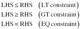
Constraints appear in three varieties in optimization models: less-than (LT) constraints, greaterthan (GT) constraints, and equal-to (EQ) constraints. Each constraint involves a relationship between a left-hand side (LHS) and a right-hand side (RHS) By convention, the RHS is a number (usually a parameter), and the LHS is a function of the decision variables. The forms of the three varieties are:
We use LT constraints to represent capacities or ceilings, GT constraints to represent commitments or thresholds, and EQ constraints to represent material balance or consistency among related variables. Box 2.2 lists some common examples of these kinds of constraints. For an example of consistency in an EQ constraint, think about a cash-planning application involving a requirement that end-of-month cash (E) must equal start-of-month cash (S) plus collections (C) minus disbursements (D).
BOX2.2ExamplesofConstraints
Less-than constraints
Number of pounds of steel consumed ≤ number of pounds available
Number of customers serviced ≤ service capacity
Thousands of televisions sold ≤ market demand (in thousands)
Greater-than constraints
Number of cartons delivered ≥ number of cartons ordered
Number of nurses scheduled ≥ number of nurses required on duty