978-9351500827
Visit to download the full and correct content document: https://ebookmass.com/product/etextbook-978-9351500827-discovering-statistics-usi ng-ibm-spss-statistics-4th-edition/
More products digital (pdf, epub, mobi) instant download maybe you interests ...
Discovering Statistics Using IBM SPSS Statistics: North American Edition 5th Edition, (Ebook PDF)
https://ebookmass.com/product/discovering-statistics-using-ibmspss-statistics-north-american-edition-5th-edition-ebook-pdf/
Statistics Using IBM SPSS: An Integrative Approach –Ebook PDF Version
https://ebookmass.com/product/statistics-using-ibm-spss-anintegrative-approach-ebook-pdf-version/
Using IBM SPSS Statistics: An Interactive Hands On Approach 3rd Edition, (Ebook PDF)
https://ebookmass.com/product/using-ibm-spss-statistics-aninteractive-hands-on-approach-3rd-edition-ebook-pdf/
Introductory Statistics Using SPSS 2nd Edition, (Ebook PDF)
https://ebookmass.com/product/introductory-statistics-usingspss-2nd-edition-ebook-pdf/
eTextbook 978-0134173054 Statistics for Managers Using Microsoft Excel
https://ebookmass.com/product/etextbook-978-0134173054statistics-for-managers-using-microsoft-excel/
A Simple Guide to IBM SPSS Statistics – version 23.0 –Ebook PDF Version
https://ebookmass.com/product/a-simple-guide-to-ibm-spssstatistics-version-23-0-ebook-pdf-version/
Practical Statistics for Nursing Using SPSS 1st Edition, (Ebook PDF)
https://ebookmass.com/product/practical-statistics-for-nursingusing-spss-1st-edition-ebook-pdf/
Using Statistics in the Social and Health Sciences with SPSS Excel 1st…
https://ebookmass.com/product/using-statistics-in-the-social-andhealth-sciences-with-spss-excel-1st/
Statistics: Informed Decisions Using Data 4th Edition, (Ebook PDF)
https://ebookmass.com/product/statistics-informed-decisionsusing-data-4th-edition-ebook-pdf/
2 Everything you never wanted to know about statistics
2.1. What will this chapter tell me? ①
2.2. Building statistical models ①
2.3. Populations and samples ①
2.4. Statistical models ①
2.4.1. The mean as a statistical model ①
2.4.2. Assessing the fit of a model: sums of squares and variance revisited ①
2.4.3. Estimating parameters ①
2.5. Going beyond the data ①
2.5.1. The standard error ①
2.5.2. Confidence intervals ②
2.6. Using statistical models to test research questions ①
2.6.1. Null hypothesis significance testing ①
2.6.2. Problems with NHST ②
2.7. Modern approaches to theory testing ②
2.7.1. Effect sizes ②
2.7.2. Meta-analysis ②
2.8. Reporting statistical models ②
2.9. Brian’s attempt to woo Jane ①
2.10. What next? ①
2.11. Key terms that I’ve discovered 2.12. Smart Alex’s tasks
2.13. Further reading
3 The IBM SPSS Statistics environment
3.1. What will this chapter tell me? ①
3.2. Versions of IBM SPSS Statistics ①
3.3. Windows versus MacOS ①
3.4. Getting started ①
3.5. The data editor ①
3.5.1. Entering data into the data editor ①
3.5.2. The variable view ①
3.5.3. Missing values ①
3.6. Importing data ①
3.7. The SPSS viewer ①
3.8. Exporting SPSS output ①
3.9. The syntax editor ③
3.10. Saving files ①
3.11. Retrieving a file ①
3.12. Brian’s attempt to woo Jane ①
3.13. What next? ①
3.14. Key terms that I’ve discovered
3.15. Smart Alex’s tasks
3.16. Further reading
4 Exploring data with graphs
4.1. What will this chapter tell me? ①
4.2. The art of presenting data ①
4.2.1. What makes a good graph? ①
4.2.2. Lies, damned lies, and … erm … graphs ①
4.3. The SPSS chart builder ①
4.4. Histograms ①
4.5. Boxplots (box–whisker diagrams) ①
4.6. Graphing means: bar charts and error bars ①
4.6.1. Simple bar charts for independent means ①
4.6.2. Clustered bar charts for independent means ①
4.6.3. Simple bar charts for related means ①
4.6.4. Clustered bar charts for related means ①
4.6.5. Clustered bar charts for ‘mixed’designs ①
4.7. Line charts ①
4.8. Graphing relationships: the scatterplot ①
4.8.1. Simple scatterplot ①
4.8.2. Grouped scatterplot ①
4.8.3. Simple and grouped 3-D scatterplots ①
4.8.4. Matrix scatterplot ①
4.8.5. Simple dot plot or density plot ①
4.8.6. Drop-line graph ①
4.9. Editing graphs ①
4.10. Brian’s attempt to woo Jane ①
4.11. What next? ①
4.12. Key terms that I’ve discovered
4.13. Smart Alex’s tasks
4.14. Further reading
5 The beast of bias
5.1. What will this chapter tell me? ①
5.2. What is bias? ①
5.2.1. Assumptions ①
5.2.2. Outliers ①
5.2.3. Additivity and linearity ①
5.2.4. Normally distributed something or other ①
5.2.5. Homoscedasticity/homogeneity of variance ②
5.2.6. Independence ②
5.3 Spotting bias ②
5.3.1. Spotting outliers ②
5.3.2. Spotting normality ①
5.3.3. Spotting linearity and heteroscedasticity/heterogeneity of variance ②
5.4. Reducing bias ②
5.4.1. Trimming the data ②
5.4.2. Winsorizing ①
5.4.3. Robust methods ③
5.4.4. Transforming data ②
5.5. Brian’s attempt to woo Jane ①
5.6. What next? ①
5.7. Key terms that I’ve discovered
5.8. Smart Alex’s tasks
5.9. Further reading
6 Non-parametric models
6.1. What will this chapter tell me? ①
6.2. When to use non-parametric tests ①
6.3. General procedure of non-parametric tests in SPSS ①
6.4. Comparing two independent conditions: the Wilcoxon rank-sum test and Mann–Whitney test ①
6.4.1. Theory ②
6.4.2. Inputting data and provisional analysis ①
6.4.3. The Mann–Whitney test using SPSS ①
6.4.4. Output from the Mann–Whitney test ①
6.4.5. Calculating an effect size ②
6.4.6. Writing the results ①
6.5. Comparing two related conditions: the Wilcoxon signed-rank test ①
6.5.1. Theory of the Wilcoxon signed-rank test ②
6.5.2. Running the analysis ①
6.5.3. Output for the ecstasy group ①
6.5.4. Output for the alcohol group ①
6.5.5. Calculating an effect size ②
6.5.6. Writing the results ①
6.6. Differences between several independent groups: the Kruskal–Wallis test ①
6.6.1. Theory of the Kruskal–Wallis test ②
6.6.2. Follow-up analysis ②
6.6.3. Inputting data and provisional analysis ①
6.6.4. Doing the Kruskal–Wallis test in SPSS ①
6.6.5. Output from the Kruskal–Wallis test ①
6.6.6. Testing for trends: the Jonckheere–Terpstra test ②
6.6.7. Calculating an effect size ②
6.6.8. Writing and interpreting the results ①
6.7. Differences between several related groups: Friedman’s ANOVA ①
6.7.1. Theory of Friedman’s ANOVA ②
6.7.2. Inputting data and provisional analysis ①
6.7.3. Doing Friedman’s ANOVA in SPSS ①
6.7.4. Output from Friedman’s ANOVA ①
6.7.5. Following-up Friedman’s ANOVA ②
6.7.6. Calculating an effect size ②
6.7.7. Writing and interpreting the results ①
6.8. Brian’s attempt to woo Jane ①
6.9. What next? ①
6.10. Key terms that I’ve discovered
6.11. Smart Alex’s tasks
6.12. Further reading
7 Correlation
7.1. What will this chapter tell me? ①
7.2. Modelling relationships ①
7.2.1. A detour into the murky world of covariance ①
7.2.2. Standardization and the correlation coefficient ①
7.2.3. The significance of the correlation coefficient ③
7.2.4. Confidence intervals for r ③
7.2.5. A word of warning about interpretation: causality ①
7.3. Data entry for correlation analysis using SPSS ①
7.4. Bivariate correlation ①
7.4.1. General procedure for running correlations in SPSS ①
7.4.2. Pearson’s correlation coefficient ①
7.4.3. Spearman’s correlation coefficient ①
7.4.4. Kendall’s tau (non-parametric) ①
7.4.5. Biserial and point-biserial correlations ③
7.5. Partial correlation ②
7.5.1. The theory behind part and partial correlation ③
7.5.2. Partial correlation in SPSS ③
7.5.3. Semi-partial (or part) correlations ②
7.6. Comparing correlations ③
7.6.1. Comparing independent rs ③
7.6.2. Comparing dependent rs ③
7.7. Calculating the effect size ①
7.8. How to report correlation coefficients ①
7.9. Brian’s attempt to woo Jane ①
7.10. What next? ①
7.11. Key terms that I’ve discovered
7.12. Smart Alex’s tasks
7.13. Further reading
8 Regression
8.1. What will this chapter tell me? ①
8.2. An introduction to regression ①
8.2.1. The simple linear model ①
8.2.2. The linear model with several predictors ②
8.2.3. Estimating the model ②
8.2.4. Assessing the goodness of fit, sums of squares, R and R2 ①
8.2.5. Assessing individual predictors ①
8.3. Bias in regression models? ②
8.3.1. Is the model biased by unusual cases? ②
8.3.2. Generalizing the model ②
8.3.3. Sample size in regression ③
8.4. Regression using SPSS: One Predictor ①
8.4.1. Regression: the general procedure ①
8.4.2. Running a simple regression using SPSS ①
8.4.3. Interpreting a simple regression ①
8.4.4. Using the model ①
8.5. Multiple regression ②
8.5.1. Methods of regression ②
8.5.2. Comparing models ②
8.5.3. Multicollinearity ②
8.6. Regression with several predictors using SPSS ②
8.6.1. Main options ②
8.6.2. Statistics ②
8.6.3. Regression plots ②
8.6.4. Saving regression diagnostics ②
8.6.5. Further options ②
8.6.6. Robust regression ②
8.7. Interpreting multiple regression ②
8.7.1. Descriptives ②
8.7.2. Summary of model ②
8.7.3. Model parameters ②
8.7.4. Excluded variables ②
8.7.5. Assessing multicollinearity ②
8.7.6. Bias in the model: casewise diagnostics ②
8.7.7. Bias in the model: assumptions ②
8.8. What if I violate an assumption? Robust regression ②
8.9. How to report multiple regression ②
8.10. Brian’s attempt to woo Jane ①
8.11. What next? ①
8.12. Key terms that I’ve discovered
8.13. Smart Alex’s tasks
8.14. Further reading
9 Comparing two means
9.1. What will this chapter tell me? ①
9.2. Looking at differences ①
9.2.1. An example: are invisible people mischievous? ①
9.2.2. Categorical predictors in the linear model ①
9.3. The t-test ①
9.3.1. Rationale for the t-test ①
9.3.2. The independent t-test equation explained ①
9.3.3. The paired-samples t-test equation explained ①
9.4. Assumptions of the t-test ①
9.5. The independent t-test using SPSS ①
9.5.1. The general procedure ①
9.5.2. Exploring data and testing assumptions ①
9.5.3. Compute the independent t-test ①
9.5.4. Output from the independent t-test ①
9.5.5. Calculating the effect size ②
9.5.6. Reporting the independent t-test ①
9.6. Paired-samples t-test using SPSS ①
9.6.1. Entering data ①
9.6.2. Exploring data and testing assumptions ①
9.6.3. Computing the paired-samples t-test ①
9.6.4. Calculating the effect size ①
9.6.5. Reporting the paired-samples t-test ①
9.7. Between groups or repeated measures? ①
9.8. What if I violate the test assumptions? ②
9.9. Brian’s attempt to woo Jane ①
9.10. What next? ①
9.11. Key terms that I’ve discovered
9.12. Smart Alex’s tasks
9.13. Further reading
10 Moderation, mediation and more regression
10.1. What will this chapter tell me? ①
10.2. Installing custom dialog boxes in SPSS ②
10.3. Moderation: interactions in regression ③
10.3.1. The conceptual model ③
10.3.2. The statistical model ②
10.3.3. Centring variables ②
10.3.4. Creating interaction variables ②
10.3.5. Following up an interaction effect ②
10.3.6. Running the analysis ②
10.3.7. Output from moderation analysis ②
10.3.8. Reporting moderation analysis ②
10.4. Mediation ②
10.4.1. The conceptual model ②
10.4.2. The statistical model ②
10.4.3. Effect sizes of mediation ③
10.4.4. Running the analysis ②
10.4.5. Output from mediation analysis ②
10.4.6. Reporting mediation analysis ②
10.5. Categorical predictors in regression ③
10.5.1. Dummy coding ③
10.5.2. SPSS output for dummy variables ③
10.6. Brian’s attempt to woo Jane ①
10.7. What next? ①
10.8. Key terms that I’ve discovered
10.9. Smart Alex’s tasks
10.10. Further reading
11 Comparing several means: ANOVA (GLM 1)
11.1. What will this chapter tell me? ①
11.2. The theory behind ANOVA ②
11.2.1. Using a linear model to compare means ②
11.2.2. Logic of the F-ratio ②
11.2.3. Total sum of squares (SST) ②
11.2.4. Model sum of squares (SSM) ②
11.2.5. Residual sum of squares (SSR) ②
11.2.6. Mean squares ②
11.2.7. The F-ratio ②
11.2.8. Interpreting F ②
11.3. Assumptions of ANOVA ③
11.3.1. Homogeneity of variance ②
11.3.2. Is ANOVA robust? ③
11.3.3. What to do when assumptions are violated ②
11.4. Planned contrasts ②
11.4.1. Choosing which contrasts to do ②
11.4.2. Defining contrasts using weights ②
11.4.3. Non-orthogonal comparisons ②
11.4.4. Standard contrasts ②
11.4.5. Polynomial contrasts: trend analysis ②
11.5. Post hoc procedures ②
11.5.1. Type I and Type II error rates for post hoc tests ②
11.5.2. Are post hoc procedures robust? ②
11.5.3. Summary of post hoc procedures ②
11.6. Running one-way ANOVA in SPSS ②
11.6.1. General procedure of one-way ANOVA ②
11.6.2. Planned comparisons using SPSS ②
11.6.3. Post hoc tests in SPSS ②
11.6.4. Options ②
11.6.5. Bootstrapping ②
11.7. Output from one-way ANOVA ②
11.7.1. Output for the main analysis ②
11.7.2. Output for planned comparisons ②
11.7.3. Output for post hoc tests ②
11.8. Calculating the effect size ②
11.9. Reporting results from one-way independent ANOVA ②
11.10. Key terms that I’ve discovered
11.11. Brian’s attempt to woo Jane ①
11.12. What next? ①
11.13. Smart Alex’s tasks
11.14. Further reading
12 Analysis of covariance, ANCOVA (GLM 2)
12.1. What will this chapter tell me? ②
12.2. What is ANCOVA? ②
12.3. Assumptions and issues in ANCOVA ③
12.3.1. Independence of the covariate and treatment effect ③
12.3.2. Homogeneity of regression slopes ③
12.3.3. What to do when assumptions are violated ②
12.4. Conducting ANCOVA in SPSS ②
12.4.1. General procedure ①
12.4.2. Inputting data ①
12.4.3. Testing the independence of the treatment variable and covariate ②
12.4.4. The main analysis ②
12.4.5. Contrasts
12.4.6. Other options ②
12.4.7. Bootstrapping and plots ②
12.5. Interpreting the output from ANCOVA ②
12.5.1. What happens when the covariate is excluded? ②
12.5.2. The main analysis ②
12.5.3. Contrasts ②
12.5.4. Interpreting the covariate ②
12.6. Testing the assumption of homogeneity of regression slopes ③
12.7. Calculating the effect size ②
12.8. Reporting results ②
12.9. Brian’s attempt to woo Jane ①
12.10. What next? ②
12.11. Key terms that I’ve discovered
12.12. Smart Alex’s tasks
12.13. Further reading
13 Factorial ANOVA (GLM 3)
13.1. What will this chapter tell me? ②
13.2. Theory of factorial ANOVA (independent designs) ②
13.2.1. Factorial designs ②
13.2.2. Guess what? Factorial ANOVA is a linear model ③
13.2.3. Two-way ANOVA: behind the scenes ②
13.2.4. Total sums of squares (SST)②
13.2.5. Model sum of squares, SSM②
13.2.6. The residual sum of squares, SSR②
13.2.7. The F-ratios ②
13.3. Assumptions of factorial ANOVA ③
13.4. Factorial ANOVA using SPSS ②
13.4.1. General procedure for factorial ANOVA ①
13.4.2. Entering the data and accessing the main dialog box ②
13.4.3. Graphing interactions ②
13.4.4. Contrasts ②
13.4.5. Post hoc tests ②
13.4.6. Bootstrapping and other options ②
13.5. Output from factorial ANOVA ②
13.5.1. Levene’s test ②
13.5.2. The main ANOVA table ②
13.5.3. Contrasts ②
13.5.4. Simple effects analysis ③
13.5.5. Post hoc analysis ②
13.6. Interpreting interaction graphs ②
13.7. Calculating effect sizes ③
13.8. Reporting the results of two-way ANOVA ②
13.9. Brian’s attempt to woo Jane ① 13.10. What next? ②
13.11. Key terms that I’ve discovered
13.12. Smart Alex’s tasks
14 Repeated-measures designs (GLM 4)
14.1. What will this chapter tell me? ②
14.2. Introduction to repeated-measures designs ②
14.2.1. The assumption of sphericity ②
14.2.2. How is sphericity measured? ②
14.2.3. Assessing the severity of departures from sphericity ②
14.2.4. What is the effect of violating the assumption of sphericity? ③
14.2.5. What do you do if you violate sphericity? ②
14.3. Theory of one-way repeated-measures ANOVA ②
14.3.1. The total sum of squares, SST②
14.3.2. The within-participant sum of squares, SSW②
14.3.3. The model sum of squares, SSM②
14.3.4. The residual sum of squares, SSR②
14.3.5. The mean squares ②
14.3.6. The F-ratio ②
14.3.7. The between-participants sum of squares ②
14.4. Assumptions in repeated-measures ANOVA ③
14.5. One-way repeated-measures ANOVA using SPSS ②
14.5.1. Repeated-measures ANOVA: the general procedure ②
14.5.2. The main analysis ②
14.5.3. Defining contrasts for repeated measures ②
14.5.4. Post hoc tests and additional options ③
14.6. Output for one-way repeated-measures ANOVA ②
14.6.1. Descriptives and other diagnostics ①
14.6.2. Assessing and correcting for sphericity: Mauchly’s test ②
14.6.3. The main ANOVA ②
14.6.4. Contrasts ②
14.6.5. Post hoc tests ②
14.7. Effect sizes for repeated-measures ANOVA ③
14.8. Reporting one-way repeated-measures ANOVA ②
14.9. Factorial repeated-measures designs ②
14.9.1. The main analysis ②
14.9.2. Contrasts ②
14.9.3. Simple effects analysis ③
14.9.4. Graphing interactions ②
14.9.5. Other options ②
14.10. Output for factorial repeated-measures ANOVA ②
14.10.1. Descriptives and main analysis ②
14.10.2. Contrasts for repeated-measures variables ②
14.11. Effect sizes for factorial repeated-measures ANOVA ③
14.12. Reporting the results from factorial repeated-measures ANOVA ②
14.13. Brian’s attempt to woo Jane ①
14.14. What next? ②
14.15. Key terms that I’ve discovered
14.16. Smart Alex’s tasks
14.17. Further reading
15 Mixed design ANOVA (GLM 5)
15.1 What will this chapter tell me? ①
15.2. Mixed designs ②
15.3. Assumptions in mixed designs ②
15.4. What do men and women look for in a partner? ②
15.5. Mixed ANOVA in SPSS ②
15.5.1. Mixed ANOVA: the general procedure ②
15.5.2. Entering data ②
15.5.3. The main analysis ②
15.5.4. Other options ②
15.6. Output for mixed factorial ANOVA ③
15.6.1. The main effect of gender ②
15.6.2. The main effect of looks ②
15.6.3. The main effect of charisma ②
15.6.4. The interaction between gender and looks ②
15.6.5. The interaction between gender and charisma ②
15.6.6. The interaction between attractiveness and charisma ②
15.6.7. The interaction between looks, charisma and gender ③
15.6.8. Conclusions ③
15.7. Calculating effect sizes ③
15.8. Reporting the results of mixed ANOVA ②
15.9. Brian’s attempt to woo Jane ①
15.10. What next? ②
15.11. Key terms that I’ve discovered
15.12. Smart Alex’s tasks
15.13. Further reading
16 Multivariate analysis of variance (MANOVA)
16.1. What will this chapter tell me? ②
16.2. When to use MANOVA ②
16.3. Introduction
16.3.1. Similarities to and differences from ANOVA ②
16.3.2. Choosing outcomes ②
16.3.3. The example for this chapter ②
16.4. Theory of MANOVA ③
16.4.1. Introduction to matrices ③
16.4.2. Some important matrices and their functions ③
16.4.3. Calculating MANOVA by hand: a worked example ③
16.4.4. Principle of the MANOVA test statistic ④
16.5. Practical issues when conducting MANOVA ③
16.5.1. Assumptions and how to check them ③
16.5.2. What to do when assumptions are violated ③
16.5.3. Choosing a test statistic ③
16.5.4. Follow-up analysis ③
16.6. MANOVA using SPSS ②
16.6.1. General procedure of one-way ANOVA ②
16.6.2. The main analysis ②
16.6.3. Multiple comparisons in MANOVA ②
16.6.4. Additional options ③
16.7. Output from MANOVA ③
16.7.1. Preliminary analysis and testing assumptions ③
16.7.2. MANOVA test statistics ③
16.7.3. Univariate test statistics ②
16.7.4. SSCP matrices ③
16.7.5. Contrasts ③
16.8. Reporting results from MANOVA ②
16.9. Following up MANOVA with discriminant analysis ③
16.10. Output from the discriminant analysis ④
16.11. Reporting results from discriminant analysis ②
16.12. The final interpretation ④
16.13. Brian’s attempt to woo Jane ①
16.14. What next? ②
16.15. Key terms that I’ve discovered
16.16. Smart Alex’s tasks
16.17. Further reading
17 Exploratory factor analysis
17.1. What will this chapter tell me? ①
17.2. When to use factor analysis ②
17.3. Factors and components ②
17.3.1. Graphical representation ②
17.3.2. Mathematical representation ②
17.3.3. Factor scores ②
17.4. Discovering factors ②
17.4.1. Choosing a method ②
17.4.2. Communality ②
17.4.3. Factor analysis or PCA? ②
17.4.4. Theory behind PCA ③
17.4.5. Factor extraction: eigenvalues and the scree plot ②
17.4.6. Improving interpretation: factor rotation ③
17.5. Research example ②
17.5.1. General procedure ①
17.5.2. Before you begin ②
17.6. Running the analysis ②
17.6.1. Factor extraction in SPSS ②
17.6.2. Rotation ②
17.6.3. Scores ②
17.6.4. Options ②
17.7. Interpreting output from SPSS ②
17.7.1. Preliminary analysis ②
17.7.2. Factor extraction ②
17.7.3. Factor rotation ②
17.7.4. Factor scores ②
17.7.5. Summary ②
17.8. How to report factor analysis ①
17.9. Reliability analysis ②
17.9.1. Measures of reliability ③
17.9.2. Interpreting Cronbach’s a (some cautionary tales) ②
17.9.3. Reliability analysis in SPSS ②
17.9.4. Reliability analysis output ②
17.10. How to report reliability analysis ②
17.11. Brian’s attempt to woo Jane ①
17.12. What next? ②
17.13. Key terms that I’ve discovered
17.14. Smart Alex’s tasks
17.15. Further reading
18 Categorical data
18.1. What will this chapter tell me? ①
18.2. Analysing categorical data ①
18.3. Theory of analysing categorical data ①
18.3.1. Pearson’s chi-square test ①
18.3.2. Fisher’s exact test ①
18.3.3. The likelihood ratio ②
18.3.4. Yates’s correction ②
18.3.5. Other measures of association ①
18.3.6. Several categorical variables: loglinear analysis ③
18.4. Assumptions when analysing categorical data ①
18.4.1. Independence ①
18.4.2. Expected frequencies ①
18.4.3. More doom and gloom ①
18.5. Doing chi-square in SPSS ①
18.5.1. General procedure for analysing categorical outcomes ①
18.5.2. Entering data ①
18.5.3. Running the analysis ①
18.5.4. Output for the chi-square test ①
18.5.5. Breaking down a significant chi-square test with standardized residuals ②
18.5.6. Calculating an effect size ②
18.5.7. Reporting the results of chi-square ①
18.6. Loglinear analysis using SPSS ②
18.6.1. Initial considerations ②
18.6.2. Running loglinear analysis ②
18.6.3. Output from loglinear analysis ③
18.6.4. Following up loglinear analysis ②
18.7. Effect sizes in loglinear analysis ②
18.8. Reporting the results of loglinear analysis ②
18.9. Brian’s attempt to woo Jane ①
18.10. What next? ①
18.11. Key terms that I’ve discovered
18.12. Smart Alex’s tasks
18.13. Further reading
19 Logistic regression
19.1. What will this chapter tell me? ①
19.2. Background to logistic regression ①
19.3. What are the principles behind logistic regression? ③
19.3.1. Assessing the model: the log-likelihood statistic ③
19.3.2. Assessing the model: the deviance statistic ③
19.3.3. Assessing the model: R and R2 ③
19.3.4. Assessing the contribution of predictors: the Wald statistic ②
19.3.5. The odds ratio: exp(B) ③
19.3.6. Model building and parsimony ②
19.4. Sources of bias and common problems ④
19.4.1. Assumptions ②
19.4.2. Incomplete information from the predictors ④
19.4.3. Complete separation ④
19.4.4. Overdispersion ④
19.5. Binary logistic regression: an example that will make you feel eel ②
19.5.1. Building a model ①
19.5.2. Logistic regression: the general procedure ①
19.5.3. Data entry ①
19.5.4. Building the models in SPSS ②
19.5.5. Method of regression ②
19.5.6. Categorical predictors ②
19.5.7. Comparing the models ②
19.5.8. Rerunning the model ①
19.5.9. Obtaining residuals ②
19.5.10. Further options ②
19.5.11. Bootstrapping ②
19.6. Interpreting logistic regression ②
19.6.1. Block 0 ②
19.6.2. Model summary ②
19.6.3. Listing predicted probabilities ②
19.6.4. Interpreting residuals ②
19.6.5. Calculating the effect size ②
19.7. How to report logistic regression ②
19.8. Testing assumptions: another example ②
19.8.1. Testing for linearity of the logit ③
19.8.2. Testing for multicollinearity ③
19.9. Predicting several categories: multinomial logistic regression ③
19.9.1. Running multinomial logistic regression in SPSS ③
19.9.2. Statistics ③
19.9.3. Other options ③
19.9.4. Interpreting the multinomial logistic regression output ③
19.9.5. Reporting the results ②
19.10. Brian’s attempt to woo Jane ①
19.11. What next? ①
19.12. Key terms that I’ve discovered
19.13. Smart Alex’s tasks
19.14. Further reading
20 Multilevel linear models
20.1. What will this chapter tell me? ①
20.2. Hierarchical data ②
20.2.1. The intraclass correlation ②
20.2.2. Benefits of multilevel models ②
20.3 Theory of multilevel linear models ③
20.3.1. An example ②
20.3.2. Fixed and random coefficients ③
20.4 The multilevel model ④
20.4.1. Assessing the fit and comparing multilevel models ④
20.4.2. Types of covariance structures ④
20.5 Some practical issues ③
20.5.1. Assumptions ③
20.5.2. Robust multilevel models ③
20.5.3. Sample size and power ③
20.5.4. Centring predictors ③
20.6 Multilevel modelling using SPSS ④
20.6.1. Entering the data ②
20.6.2. Ignoring the data structure: ANOVA ②
20.6.3. Ignoring the data structure: ANCOVA ②
20.6.4. Factoring in the data structure: random intercepts ③
20.6.5. Factoring in the data structure: random intercepts and slopes ④
20.6.6. Adding an interaction to the model ④
20.7. Growth models ④
20.7.1. Growth curves (polynomials) ④
20.7.2. An example: the honeymoon period ②
20.7.3. Restructuring the data ③
20.7.4. Running a growth model on SPSS ④
20.7.5. Further analysis ④
20.8. How to report a multilevel model ③
20.9. A message from the octopus of inescapable despair ①
20.10. Brian’s attempt to woo Jane ①
20.11. What next? ②
20.12. Key terms that I’ve discovered
20.13. Smart Alex’s tasks
20.14. Further reading
21 Epilogue: life after discovering statistics
21.1. Nice emails
21.2. Everybody thinks that I’m a statistician
21.3. Craziness on a grand scale
21.3.1. Catistics
21.3.2. Cult of underlying numerical truths
21.3.3. And then it got really weird
Glossary
Appendix
References
Index
PREFACE
Karma Police, arrest this man, he talks in maths, he buzzes like a fridge, he’s like a detuned radio
Radiohead, ‘Karma Police’, OK Computer (1997)
Introduction
Many behavioural and social science students (and researchers for that matter) despise statistics. Most of us have a non-mathematical background, which makes understanding complex statistical equations very difficult. Nevertheless, the evil goat-warriors of Satan force our non-mathematical brains to apply themselves to what is the very complex task of becoming a statistics expert. The end result, as you might expect, can be quite messy. The one weapon that we have is the computer, which allows us to neatly circumvent the considerable disability of not understanding mathematics. Computer programs such as IBM SPSS Statistics, SAS, R and the like provide an opportunity to teach statistics at a conceptual level without getting too bogged down in equations. The computer to a goat-warrior of Satan is like catnip to a cat: it makes them rub their heads along the ground and purr and dribble ceaselessly. The only downside of the computer is that it makes it really easy to make a complete idiot of yourself if you don’t really understand what you’re doing. Using a computer without any statistical knowledge at all can be a dangerous thing. Hence this book.
My first aim is to strike a good balance between theory and practice: I want to use the computer as a tool for teaching statistical concepts in the hope that you will gain a better understanding of both theory and practice. If you want theory and you like equations then there are certainly better books: Howell (2012), Stevens (2002) and Tabachnick and Fidell (2012) have taught (and continue to teach) me more about statistics than you could possibly imagine. (I have an ambition to be cited in one of these books, but I don’t think that will ever happen.) However, if you want a stats book that also discusses digital rectal stimulation then you have just spent your money wisely.
Too many books create the impression that there is a ‘right’ and ‘wrong’ way to do statistics. Data analysis is more subjective than is often made out. Therefore, although I make recommendations, within the limits imposed by the senseless destruction of rainforests, I hope to give you enough background in theory to enable you to make your own decisions about how best to conduct your analysis.
A second (ridiculously ambitious) aim is to make this the only statistics book that you’ll ever need to buy. It’s a book that I hope will become your friend from first year at university right through to your professorship. The start of the book is aimed at first-year undergraduates (Chapters 1–9), and then we move onto second-year undergraduate level material (Chapters 5, 8 and 10–15) before a dramatic climax that should keep postgraduates tickled (Chapters 16–20). There should be something for everyone in each chapter also, and to help you gauge the difficulty of material, I flag the level of each section within each chapter (more on that in a moment).
My final and most important aim is to make the learning process fun. I have a sticky history with maths. This extract is from my school report at the age of 11:
The ‘27’ in the report is to say that I came equal 27th with another student out of a class of 29. That’s pretty much bottom of the class. The 43 is my exam mark as a percentage. Oh dear. Four years later (at 15) this was my school report:
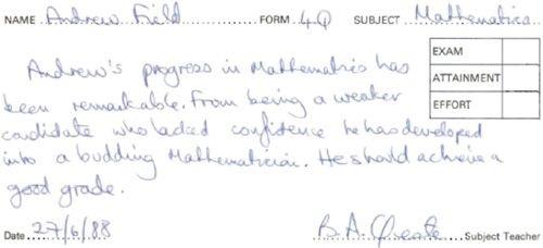
The catalyst of this remarkable change was having a good teacher: my brother, Paul. I owe my life as an academic to Paul’s ability to teach me stuff in an engaging way – something my maths teachers failed to do. Paul’s a great teacher because he cares about bringing out the best in people, and he was able to make things interesting and relevant to me. He got the ‘good teaching’ genes in the family, but wasted them by not becoming a teacher; however, they’re a little less wasted because his approach inspires mine. I strongly believe that people appreciate the human touch, and so I try to inject a lot of my own personality and sense of humour (or lack of) into Discovering Statistics Using … books. Many of the examples in this book, although inspired by some of the craziness that you find in the real world, are designed to reflect topics that play on the minds of the average student (i.e., sex, drugs, rock and roll, celebrity, people doing crazy stuff). There are also some examples that are there simply because they made me laugh. So, the examples are light-hearted (some have said ‘smutty’, but I prefer ‘lighthearted’) and by the end, for better or worse, I think you will have some idea of what goes on in my head on a daily basis. I apologize to those who think it’s crass, hate it, or think that I’m undermining the seriousness of science, but, come on, what’s not funny about a man putting an eel up his anus?
I never believe that I meet my aims, but previous editions have certainly been popular. I enjoy the rare luxury of having complete strangers emailing me to tell me how wonderful I am. (Admittedly, there are also emails calling me a pile of gibbon excrement, but you have to take the rough with the smooth.) The second edition of this book also won the British Psychological Society book award in 2007. However, with every new edition, I fear that the changes I make will ruin all of my previous hard work. Let’s see what those changes are.
What do you get for your money?
This book takes you on a journey (and I try my best to make it a pleasant one) not just of statistics but also of the weird and wonderful contents of the world and my brain. It’s full of daft, bad jokes, and smut. Aside from the smut, I have been forced reluctantly to include some academic content. In essence it contains everything I know about statistics (actually, more than I know …). It also has these features:
Everything you’ll ever need to know: I want this book to be good value for money, so it guides you from complete ignorance (Chapter 1 tells you the basics of doing research) to being an expert on multilevel modelling (Chapter 20). Of course no book that it’s physically possible to lift will contain everything, but I think this one has a fair crack. It’s pretty good for developing your biceps also.
Stupid faces: You’ll notice that the book is riddled with stupid faces, some of them my own. You can find out more about the pedagogic function of these ‘characters’in the next section, but even without any useful function they’re nice to look at.
Data sets: There are about 132 data files associated with this book on the companion website. Not unusual in itself for a statistics book, but my data sets contain more sperm (not literally) than other books. I’ll let you judge for yourself whether this is a good thing.
My life story: Each chapter is book-ended by a chronological story from my life. Does this help you to learn about statistics? Probably not, but hopefully it provides some light relief between chapters.
SPSS tips: SPSS does weird things sometimes. In each chapter, there are boxes containing tips, hints and pitfalls related to SPSS.
Self-test questions: Given how much students hate tests, I thought the best way to commit commercial suicide was to liberally scatter tests throughout each chapter. These range from simple questions to test what you have just learned to going back to a technique that you read about several chapters before and applying it in a new context. All of these questions have answers to them on the companion website so that you can check on your progress.
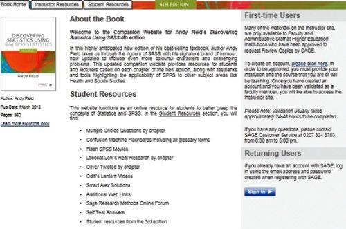
Companion website: The companion website contains an absolutely insane amount of additional material, all of which is described in the section about the companion website.
Digital stimulation: No, not the aforementioned type of digital stimulation, but brain stimulation. Many of the features on the companion website will be accessible from tablets and smartphones, so that when you’re bored in the cinema you can read about the fascinating world of heteroscedasticity instead.
Reporting your analysis: Every chapter has a guide to writing up your analysis. How you write up an analysis varies a bit from one discipline to another, but my guides should get you heading in the right direction.
Glossary: Writing the glossary was so horribly painful that it made me stick a vacuum cleaner into my ear to suck out my own brain. You can find my brain in the bottom of the vacuum cleaner in my house.
Real-world data: Students like to have ‘real data’to play with. The trouble is that real research can be quite boring. However, just for you, I trawled the world for examples of research on really fascinating topics (in my opinion). I then stalked the authors of the research until they gave me their data. Every chapter has a real research example.
What do you get that you didn’t get last time?
I suppose if you have spent your hard-earned money on the previous edition it’s reasonable that you want a good reason to spend more money on this edition. In some respects it’s hard to quantify all of the changes in a list: I’m a better writer than I was 4 year ago, so there is a lot of me rewriting things because I think I can do it better than before. I spent 6 months solidly on the updates, so suffice it to say that a lot has changed; but anything you might have liked about the previous edition probably hasn’t
changed:
IBM SPSS compliance: This edition was written using versions 20 and 21 of IBM SPSS Statistics. IBM bring out a new SPSS each year and this book gets rewritten about every 4 years, so, depending on when you buy the book, it may not reflect the latest version. This shouldn’t bother you because one edition of SPSS is usually much the same as another (see Section 3.2).
New! Mediation and Moderation: Even since the first edition I have been meaning to do a chapter on mediation and moderation, because they are two very widely used techniques. With each new edition I have run out of energy. Not this time though: I wrote it in the middle of the update before I managed to completely burn myself out. Chapter 10 is brand spanking new and all about mediation and moderation.
New! Structure: My publishers soiled their underwear at the thought of me changing the structure because they think lecturers who use the book don’t like this sort of change. They might have a point, but I changed it anyway. So, logistic regression (a complex topic) has moved towards the end of the book, and non-parametric tests (a relatively straightforward topic) have moved towards the beginning. In my opinion this change enables the book’s story to flow better.
New! Focus: Statistical times are a-changing, and people are starting to appreciate the limitations of significance testing, so I have discussed this more in Chapter 2, and the points made there permeate the rest of the book. The theme of ‘everything being the same model’has run through all editions of the book, but I have made this theme even more explicit this time.
New! Tasks: There are 111 more Smart Alex tasks, and 8 more Labcoat Leni tasks. This, of course, means there are quite a lot more pages of answers to these tasks on the companion website.
New! Bootstrapping: The SPSS bootstrapping procedure is covered in every chapter where it is relevant.
New! Process diagrams: Every chapter has a diagrammatic summary of the key steps that you go through for a particular analysis.
New! Love story: Every chapter has a diagrammatic summary at the end (Brian’s attempt to woo Jane). More interesting, though, Brian Haemorrhage has fallen in love with Jane Superbrain (see next section) and these diagrams follow Brian’s attempts to convince Jane to go on a date with him.
New! Characters: I enjoy coming up with new characters, and this edition has a crazy hippy called Oditi, and a deranged philosopher called Confusius (see the next section).
New-ish! Assumptions: I’ve never really liked the way I dealt with assumptions, so I completely rewrote Chapter 5 to try to give more of a sense of when assumptions actually matter.
Every chapter had a serious edit/rewrite, but here is a chapter-by-chapter run-down of the more substantial changes:
Chapter 1 (Doing research): I added some more material on reporting data. I added stuff about variance and standard deviations, and expanded the discussion of p-values.
Chapter 2 (Statistical theory): I added material on estimating parameters, significance testing and its limitations, problems with one-tailed tests, running multiple tests (i.e., familywise error), confidence intervals and significance, sample size and significance, effect sizes (including Cohen’s d and meta-analysis), and reporting basic statistics. It’s changed a lot.
Chapter 3 (IBM SPSS): No dramatic changes.
Chapter 4 (Graphs): I moved the discussion of outliers into Chapter 5, which meant I had to rewrite one of the examples. I now include population pyramids also.
Chapter 5 (Assumptions): I completely rewrote this chapter. It’s still about assumptions, but I try to explain when they matter and what they bias. Rather than dealing with assumptions separately in every chapter, because everything in the book is a linear model, I deal with the assumptions of linear models here. Therefore, this chapter acts as a single reference point for all subsequent chapters. I also cover other sources of bias such as outliers (which used to be scattered about in different chapters).
Chapter 6 (Non-parametric models): This is a fully updated and rewritten chapter on nonparametric statistics. It used to be later in the book, but now flows gracefully on from the discussion of assumptions.
Chapter 7 (Correlation): No dramatic changes.
Chapter 8 (Regression): I restructured this chapter so that most of the theory is now at the beginning and most of the SPSS is at the end. I did a fair bit of editing, too, moved categorical predictors into Chapter 10, and integrated simple and multiple regression more.
Chapter 9 (t-tests): The old version of this chapter used spider examples, but someone emailed me to say that this freaked them out, so I changed the example to be about cloaks of invisibility. Hopefully that won’t freak anyone out. I restructured a bit, too, so that the theory is in one place and the SPSS in another.
Chapter 10 (Mediation and moderation): This chapter is completely new.
Chapter 11 (GLM 1): I gave more prominence to ANOVA as a general linear model because this makes it easier to think about assumptions and bias. I moved some of the more technical bits of the SPSS interpretation into boxes so that you can ignore them if you wish.
Chapter 12 (GLM 2): Again some restructuring and a bit more discussion on whether the covariate and predictor need to be independent.
Chapters 13–15 (GLM 3–5): These haven’t changed much. I restructured each one a bit, edited down/rewrote a lot and gave more prominence to the GLM way of thinking.
Chapter 16 (MANOVA): I gave the writing a bit of a polish, but no real content changes.
Chapter 17 (Factor analysis): I added some stuff to the theory to make the distinction between principal component analysis (PCA) and factor analysis (FA) clearer. The chapter used to focus on PCA, but I changed it so that the focus is on FA. I edited out 3000 words of my tedious, repetitive, superfluous drivel.
Chapters 18 and 19 (Categorical data and logistic regression): Because these chapters both deal with categorical outcomes, I rewrote them and put them together. The basic content is the same as before.
Chapter 20 (Multilevel models): I polished the writing a bit and updated, but there are no changes that will upset anyone.
Goodbye
The first edition of this book was the result of two years (give or take a few weeks to write up my Ph.D.) of trying to write a statistics book that I would enjoy reading. With each new edition I try not just to make superficial changes but also to rewrite and improve everything (one of the problems with getting older is you look back at your past work and think you can do things better). This fourth edition is the culmination of about 6 years of full-time work (on top of my actual job). This book has literally consumed the last 15 years or so of my life, and each time I get a nice email from someone who found it useful I am reminded that it is the most useful thing I’ll ever do with my life. It began and continues to
be a labour of love. It still isn’t perfect, and I still love to have feedback (good or bad) from the people who matter most: you.
HOW TO USE THIS BOOK
When the publishers asked me to write a section on ‘How to use this book’ it was tempting to write ‘Buy a large bottle of Olay anti-wrinkle cream (which you’ll need to fend off the effects of ageing while you read), find a comfy chair, sit down, fold back the front cover, begin reading and stop when you reach the back cover.’However, I think they wanted something more useful.
What background knowledge do I need?
In essence, I assume that you know nothing about statistics, but that you have a very basic grasp of computers (I won’t be telling you how to switch them on, for example) and maths (although I have included a quick revision of some very basic concepts, so I really don’t assume much).
Do the chapters get more difficult as I go through the book?
Yes, more or less: Chapters 1–9 are first-year degree level, Chapters 8–15 move into second-year degree level, and Chapters 16–20 discuss more technical topics. However, my main aim is to tell a statistical story rather than worrying about what level a topic is at. Many books teach different tests in isolation and never really give you a grasp of the similarities between them; this, I think, creates an unnecessary mystery. Most of the tests in this book are the same thing expressed in slightly different ways. I want the book to tell this story, and I see it as consisting of seven parts:
Part 1 (Doing research and introducing linear models): Chapters 1–3.
Part 2 (Exploring data): Chapters 4–6.
Part 3 (Linear models with continuous predictors): Chapters 7 and 8.
Part 4 (Linear models with continuous or categorical predictors): Chapters 9–15.
Part 5 (Linear models with multiple outcomes): Chapter 16 and 17.
Part 6 (Linear models with categorical outcomes): Chapters 18–19.
Part 7 (Linear models with hierarchical data structures): Chapter 20.
This structure might help you to see the method in my madness. If not, to help you on your journey I’ve coded each section with an icon. These icons are designed to give you an idea of the difficulty of the section. It doesn’t mean you can skip the sections (but see Smart Alex in the next section), but it will let you know whether a section is at about your level, or whether it’s going to push you. It’s based on a wonderful categorization system using the letter ‘I’:
① Introductory, which I hope means that everyone should be able to understand these sections. These are for people just starting their undergraduate courses.
② Intermediate. Anyone with a bit of background in statistics should be able to get to grips with these sections. They are aimed at people who are perhaps in the second year of their degree, but they can still be quite challenging in places.
③ In at the deep end. These topics are difficult. I’d expect final-year undergraduates and recent postgraduate students to be able to tackle these sections.
④ Incinerate your brain. These are difficult topics. I would expect these sections to be challenging for undergraduates, but postgraduates with a reasonable background in research methods shouldn’t find them too much of a problem.
Why do I keep seeing silly faces everywhere?

Brian Haemorrhage: Brian is a really nice guy, and he has a massive crush on Jane Superbrain. He’s seen her around the university campus carrying her jars of brains (see below). Whenever he sees her, he gets a knot in his stomach and he imagines slipping a ring onto her finger on a beach in Hawaii, as their friends and family watch through their gooey eyes. Jane never even notices him; this makes him very sad. His friends have told him that the only way she’ll marry him is if he becomes a statistics genius (and changes his surname). Therefore, he’s on a mission to learn statistics. It’s his last hope of impressing Jane, settling down and living happily ever after. At the moment he knows nothing, but he’s about to embark on a journey that will take him from statistically challenged to a genius, in 900 pages. Along his journey he pops up and asks questions, and at the end of each chapter he flaunts his newly found knowledge to Jane in the hope she’ll go on a date with him.
New! Confusius: The great philosopher Confucius had a lesser-known brother called Confusius. Jealous of his brother’s great wisdom and modesty, Confusius vowed to bring confusion to the world. To this end, he built the confusion machine. He puts statistical terms into it, and out of it come different names for the same concept. When you see Confusius he will be alerting you to statistical terms that mean the same thing.
Cramming Sam: Samantha thinks statistics is a boring waste of time and she just wants to pass her exam and forget that she ever had to know anything about normal distributions. She appears and gives you a summary of the key points that you need to know. If, like Samantha, you’re cramming for an exam, she will tell you the essential information to save you having to trawl through hundreds of pages of my drivel.
Curious Cat: He also pops up and asks questions (because he’s curious). The only reason he’s here is because I wanted a cat in the book … and preferably one that looks like mine. Of course the educational specialists think he needs a specific role, and so his role is to look cute and make bad cat-related jokes.
Jane Superbrain: Jane is the cleverest person in the whole universe. A mistress of osmosis, she acquired vast statistical knowledge by stealing the brains of statisticians and eating them. Apparently they taste of sweaty tank tops. Having devoured some top statistics brains and absorbed their knowledge, she knows all of the really hard stuff. She appears in boxes to tell you advanced things that are a bit tangential to the main text. Her friends tell her that a half-whit called Brian is in love with her, but she doesn’t know who he is.
Labcoat Leni: Leni is a budding young scientist and he’s fascinated by real research. He says, ‘Andy, man, I like an example about using an eel as a cure for constipation as much as the next guy, but all of your data are made up. We need some real examples, dude!’ So off Leni went: he walked the globe, a lone data warrior in a thankless quest for real data. He turned up at universities, cornered academics, kidnapped their families and threatened to put them in a bath of crayfish unless he was given real data. The generous ones relented, but others? Well, let’s just say their families are sore. So, when you see Leni you know that you will get some real data, from a real research study to analyse. Keep it real.

New! Oditi’s Lantern: Oditi believes that the secret to life is hidden in numbers and that only by largescale analysis of those numbers shall the secrets be found. He didn’t have time to enter, analyse and interpret all of the data in the world, so he established the cult of undiscovered numerical truths. Working on the principle that if you gave a million monkeys typewriters, one of them would re-create Shakespeare, members of the cult sit at their computers crunching numbers in the hope that one of them will unearth the hidden meaning of life. To help his cult Oditi has set up a visual vortex called ‘Oditi’s Lantern’. When Oditi appears it is to implore you to stare into the lantern, which basically means there is a video tutorial to guide you.

Oliver Twisted: With apologies to Charles Dickens, Oliver, like the more famous fictional London urchin, is always asking ‘Please, Sir, can I have some more?’ Unlike Master Twist though, our young Master Twisted wants more statistics information. Of course he does, who wouldn’t? Let us not be the ones to disappoint a young, dirty, slightly smelly boy who dines on gruel. When Oliver appears he’s telling you that there is additional information to be found on the companion website. (It took a long time to write, so someone please actually read it.)

Satan’s Personal Statistics Slave: Satan is a busy boy – he has all of the lost souls to torture in hell; then there are the fires to keep fuelled, not to mention organizing enough carnage on the planet’s surface to keep Norwegian black metal bands inspired. Like many of us, this leaves little time for him to analyse data, and this makes him very sad. So, he has his own personal slave, who, also like some of us, spends all day dressed in a gimp mask and tight leather pants in front of IBM SPSS analysing Satan’s data. Consequently, he knows a thing or two about SPSS, and when Satan’s busy spanking a goat, he pops up in a box with SPSS tips.
Smart Alex: Alex is a very important character because he appears when things get particularly difficult. He’s basically a bit of a smart alec, and so whenever you see his face you know that something scary is about to be explained. When the hard stuff is over he reappears to let you know that it’s safe to continue. You’ll also find that Alex gives you tasks to do at the end of each chapter to see whether you’re as smart as he is.
Why do I keep seeing QR codes?
MobileStudy: QR stands for ‘quantum reality’, and if you download a QR scanner and scan one of these funny little barcode things into your mobile device (smartphone, tablet, etc…) it will transport you and your device into a quantum reality in which left is right, time runs backwards, drinks pour themselves out of your mouth into bottles, and statistics is interesting. Scanning these codes will be your gateway to revision resources such as Chapter Introductions, Cramming Sam’s Tips, Interactive Multiple Choice Questions, and more. Don’t forget to add MobileStudy to your favourites on your device so you can revise any time you like – even on the toilet!
What is on the companion website?
In this age of downloading, CD-ROMs are for losers (at least that’s what the ‘kids’ tell me), so I’ve put my cornucopia of additional funk on that worldwide interweb thing. To enter my world of delights, go to www.sagepub.co.uk/field4e. The website contains resources for students and lecturers alike, with additional content from some of the characters from the book.
Testbank: There is a comprehensive testbank of multiple choice and numeracy questions for instructors. This comes in two flavours: (1) Testbank files supporting a range of disciplines are available for lecturers to upload into their online teaching system; (2) A powerful, online, instructional tool for students and lecturers called WebAssign® . WebAssign® allows instructors to assign questions for exams and assignments which can be automatically graded for formative and summative assessment. WebAssign® also supports student revision by allowing them to learn at their own pace and practise statistical principles again and again until they master them. To further assist learning WebAssign® also gives feedback on right and wrong answers and provides students with access to an electronic version of the textbook to further their study.

Data files: You need data files to work through the examples in the book and they are all on the companion website. We did this so that you’re forced to go there and once you’re there Sage will
flash up subliminal messages to make you buy more of their books. Resources for different subject areas: I am a psychologist and although I tend to base my examples around the weird and wonderful, I do have a nasty habit of resorting to psychology when I don’t have any better ideas. I realize that not everyone is as psychologically oriented as me, so my publishers have recruited some non-psychologists to provide data files and an instructor’s testbank of multiple-choice questions for those studying or teaching in business and management, education, sport sciences and health sciences. You have no idea how happy I am that I didn’t have to write those.
Webcasts: Whenever you see Oditi in the book it means that there is a webcast to accompany the chapter. These are hosted on my YouTube channel (www.youtube.com/user/ProfAndyField), which I have amusingly called μ-Tube (see what I did there?). You can also get to them via the companion website.
Self-assessment multiple-choice questions: Organized by chapter, these will allow you to test whether wasting your life reading this book has paid off so that you can annoy your friends by walking with an air of confidence into the examination. If you fail said exam, please don’t sue me.
Flashcard glossary: As if a printed glossary wasn’t enough, my publishers insisted that you’d like an electronic one too. Have fun here flipping through terms and definitions covered in the textbook; it’s better than actually learning something.
Oliver Twisted’s pot of gruel: Oliver Twisted will draw your attention to the 300 pages or so of more technical information that we have put online so that (1) the planet suffers a little less, and (2) you won’t die when the book falls off of your bookshelf onto your head.
Labcoat Leni solutions: For all of the Labcoat Leni tasks in the book there are full and detailed answers on the companion website.
Smart Alex answers: Each chapter ends with a set of tasks for you to test your newly acquired expertise. The chapters are also littered with self-test questions. The companion website contains around 300 pages (that’s a different 300 pages to the 300 above) of detailed answers. Will I ever stop writing?
PowerPoint slides: I can’t come and teach you all in person (although you can watch my lectures on YouTube). Instead I rely on a crack team of highly skilled and super-intelligent pan-dimensional beings called ‘lecturers’. I have personally grown each and every one of them in a greenhouse in my garden. To assist in their mission to spread the joy of statistics I have provided them with PowerPoint slides for each chapter. If you see something weird on their slides that upsets you, then remember that’s probably my fault.
Links: Every website has to have links to other useful websites, and the companion website is no exception.
Cyberworms of knowledge: I have used nanotechnology to create cyberworms that crawl down your broadband connection, pop out of the USB port of your computer and fly through space into your brain. They rearrange your neurons so that you understand statistics. You don’t believe me? Well, you’ll never know for sure unless you visit the companion website ….
Happy reading, and don’t get distracted by Facebook and Twitter.