EKSEMPLER PÅ
ENERGIFLEKSIBILITETSPOTENTIALER I

AFSLUTNINGSRAPPORT CASE 1
BORNHOLMS HOSPITAL
FUTURE
– Case 2: Integration af vedvarende energi i komplekse bygninger
Ressourcer

FUTU nergiE
FUTURessourcer nergiE

1
Projektleder

Projektet er støttet af
Projektet støttes af den Europæiske Regionaludviklingsfond og Interreg ÖKS samt Region Hovedstaden, Region Sjælland og Region Skåne.

Forfattere
Janne Dragsted, Weiqiang Kong, Simon Furbo, Per Dahlgaard Pedersen
Publiceret af
FUTURE
Layout forside og bagside
Kasper Laulund Kjeldsmark (Gate 21)
2021
2
FUTURE FREMTIDENS INTELLIGENTE ENERGI- OG RESSOURCESYSTEM
FUTURE-projektet består af syv visionære casesamarbejder på tværs af de tre regioner i Greater Copenhagen. De syv cases tester og demonstrerer forskellige teknologier, værktøjer eller forretningsmodeller indenfor vedvarende energi eller udnyttelse af ressourcer:
• Case 1: Fleksibel energilagring i individuelle bygninger
• Case 2: Integration af vedvarende energi i komplekse bygninger
• Case 3: Forbedret energihusholdning gennem balanceret varme og køling i sygehusbygninger
• Case 4: Energioptimering gennem smarte grids i bygninger
• Case 5: Cirkulære løsninger, der integrerer energi, ressourcer og affald
• Case 6: Resttekstiler som en del af fremtidens byggeri
• Case 7: Intelligent brug af produktdata, der forbedrer og fremmer genbrug i cirkulære samfund
Vedvarende energi
Projektet vil:
• Udnytte, integrere og lagre vedvarende energi bedre, så vi får et mere fleksibelt energisystem
• Fremme energieffektive løsninger i bygninger
Derfor skal vi designe løsninger og infrastruktur, der kan bygge bro mellem behovet for forsyningssikkerhed på den ene side, og det faktum at vedvarende energikilder ofte fluktuerer.
Ressourceudnyttelse
Projektet vil:
• Øge ressourceeffektiviteten og skabe en cirkulær omstilling af samfundet. Vi skal forlænge levetiden af materialer, genanvende affald og rester så de indgår i nye kredsløb.
• Begrænse produktionen af jomfruelige materialer og dermed også energiforbruget
Derfor demonstrerer projektet, hvordan man lokalt kan styre produkt- og materialestrømme, så man fremmer en mere intelligent materialeanvendelse
Læs mere her: https://www.gate21.dk/future/
Introduction

FUTURE is a project funded bythe EU program Interreg and hasthe overallgoalto increase the usages of renewable energy.The projectis divided into differentcases, where case #1 focusesonstorage and smart controlsof energy systemsfor individualbuildings.
The purpose of case #1 is to testa number of differentheat pump systemsinstalled with a storage and controls, in order to support and balance the electricity consumption By utilize private dwellingsand their energysystems to decrease the fluctuation in the electricity consumption during peak hours, the usages ofrenewable energy are increased.
Case #1 will investigate theeffectsof heatpump systems installed with storage tanksin order to offer flexibility the electricitygrid.
This report givesan overview ofthe gained knowledge and conclusions fromcase #1
Content 1. Systemdescription Lolland Falster Airport 5 1.1 Airport – Lolland Falster 5 1.2 Added control system installed in the airport 9 2. Systemdescriptionprivatedwellings ............................................................ 12 2.1 House 1 12 2.2 House 2 18 2.3 House 3 22 3. Storage capacity and potential 27 3.1 Water storage..............................................................................................................................27 3.2 PCM storage 27 4. Optimised control of heatpumps 29 4.1 Introduction 29 4.2 Heat pump survey and control access 29 4.3 Flexibility 29 4.4 Value proposition 31 4.5 Optimized control 32 4.6 Results and perspectives 34 5. Conclusion 38 Appendix A 39
1. SystemdescriptionLollandFalsterAirport
In the following, the installed systemin Lolland Falster Airport is presented along with measurements from the system.Evaluation of the energy performance is given, and added control for the systemis described with the effectson the flexibility.

1.1 Airport – Lolland Falster
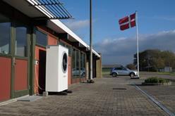
The airport in Lolland Falster is located in the southern part ofLolland. It is a commercialbuilding, with one individual working the controlsfor the runway, from8 am to 5 pm during weekdays, and no activityduring the weekend,see Figure 1.1-1.The building isa one-storeybuilding,with large glass surfacesand wooden structure.
The building consists of a control room,meeting room, canteen,kitchen, and varioussmaller utility rooms.The heating system isa water based radiator systemwith individualthermostatson the radiators.The indoor temperature sensor is placed in the control roomwhere the person working at the airport is sitting.The set pointfor the sensor is 20°C,decided bythe user.The set pointfor the radiators in the canteen and kitchen is lowered to 17 °C, since these roomsare seldomused,thisis also decided bythe user.
In Table 1.1-1 some keyparameters are given for the building and the systeminstalled at theairport. The heat loss from the building ishere not determined asdescribed in DS418,butfrom the measurements based on energydelivered to the building for space heating during stable indoor temperature periods.
5
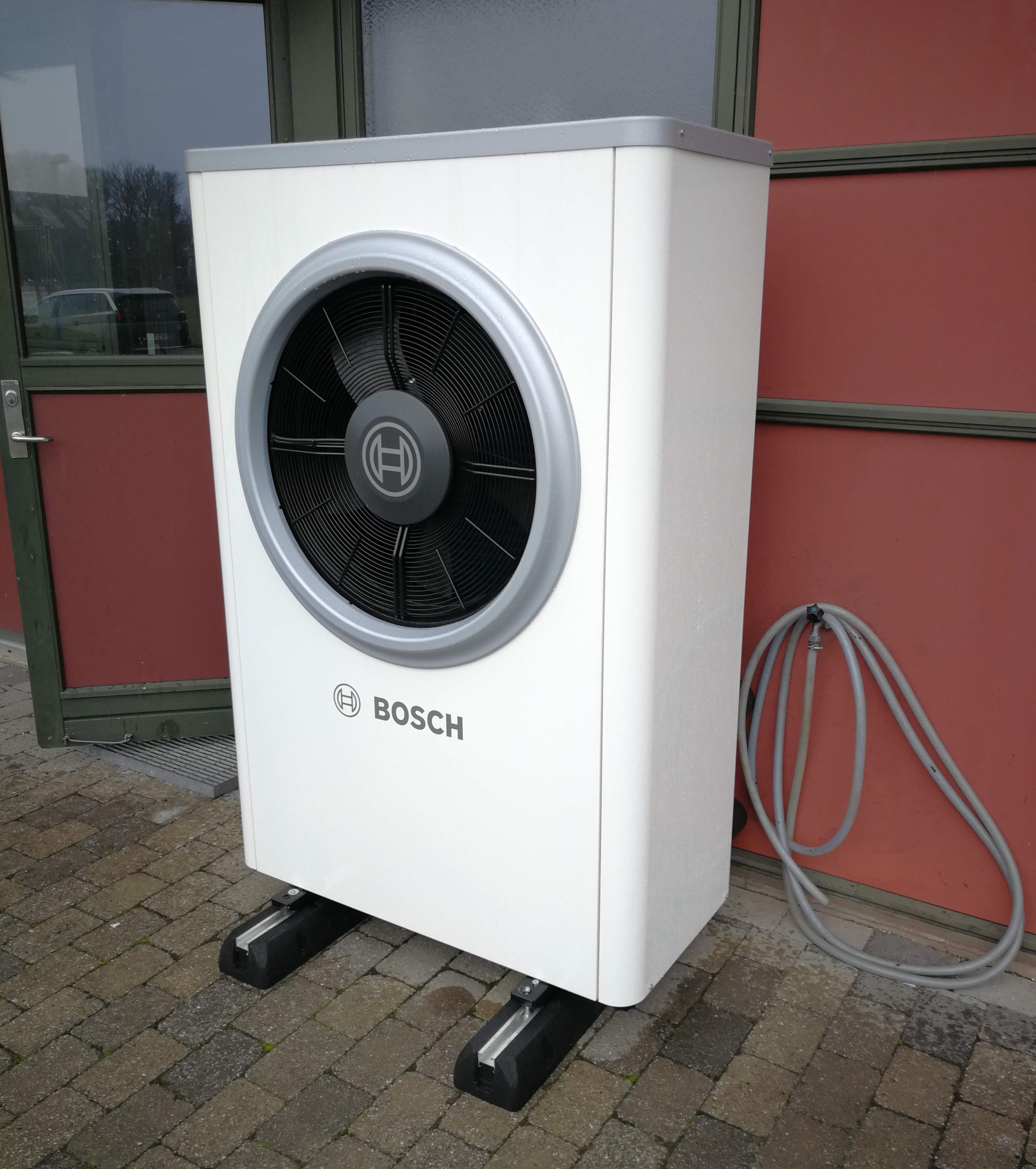
Figure 1.1-1 Aerial photo of the airport and picture of the heat pump installed at the airport.
* the building heat loss is determined based on measurements of the delivered space heating during periods with a constant indoor temperature.
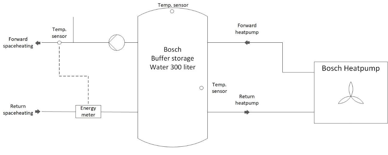
The system installed at the airport isa Bosch system,with a 13 kW heat pump and a 300 liters buffer storage,see Figure 1.1-2.The systemis onlyconnected to the space heating loop in the building, since the domestic hotwater is delivered separately, heated byan electricalheating element.
This configuration has itsadvantagesand disadvantages.It is here possible to allow the heat pump to be shut down for longer periodsand thereby lowering the temperature in the buffer storage to temperatures below domestichotwater temperatures, becauseit is not necessaryto standbywith a heated volume of hot water for domesticuse.This offersmore flexibilityin termsof the electricity used by the heatpump and a greater potential for avoiding peakhours. The disadvantages are that the domestichot water isheated by a simple heating element, which has a much lower efficiency than a heat pump. Also,the on/off controlsfor the heating element are not connected to anysmart controlsand is therebyonlycontrolled by demand.
6
Airport Lolland Falster Building area 342 [m²] Year of build 1973 [-] Building heat loss* 0.476 [kW/K] Building time constant 57 [hour] Building heat capacity 27.4 [kWh/K] Size heat pump 13 [kW] Size buffer storage (water) 300 [liters] Measurements from 1/11-2018 [dd/mm-yyyy]
Table 1.1-1 Descriptive figures for the airport
Figure 1.1-2 Diagram of the systeminstalled at airport delivered by Bosch.
Although there are disadvantagesa systemonlyconnected to the space heating loop is still very appropriate for a commercial building where the operating hoursoften for a majorityof the time is outside the morning and evening peakhours.Also,the hotwater consumption islow in smaller commercial installations where there are no shower facility and industrial kitchen activity.
Space heating
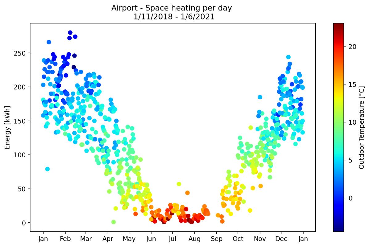
The needed energyfor space heating isgiven in Table 1.1-2. Here it is seen that the yearly consumption is between 26 MWh - 33 MWh for the measured period,dependenton the weather conditionsduring the winter.
On Figure 1.1-3 the dailyneed for space heating isgiven asa function of the time of theyear The colour indication showsthe mean daily outdoor temperature. Asexpected, the need for space heating is highestduring the winter where the outdoor temperature low.
7
Airport Lolland Falster 2018 2019 2020 2021 1/11 – 31/12 1/1 – 31/12 1/1 – 31/12 1/1 – 1/6 Degree days [-] 701 2535 2366 1774 Energy space heating [MWh] 9.84 32.77 26.32 23.87 Energy heat pump [MWh] 3.42 11.53 8.31 8.17
Table 1.1-2 Energy for space heating at the airport from the 1/11-2018 to 1/6-2021.
Figure 1.1-3 The daily need for space heating in the airport measured during the project
Performance
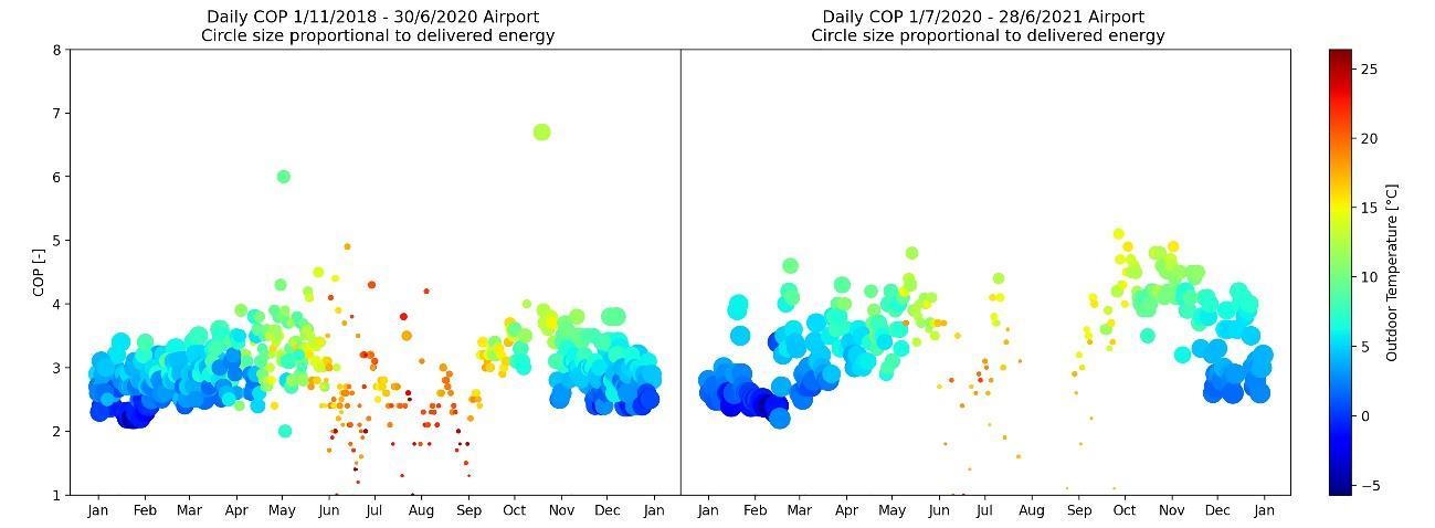
The performance of the heat pump system installed at the airport isshown on Figure 1.1-4.The figure showsthe dailyvariation over the course ofa year of the System COP, derived by the energy consumption for the heat pump and the energydelivered to the space heating loop.The size of the circle on the figure are proportional to the energy delivered,where the larger circlesare during the winter months corresponding to when the mostheat isdelivered through the space heating loop.
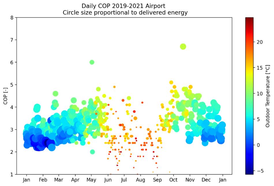
The efficiencyof the Bosch systemin the outdoor temperature interval from-5°C to 17°C is a COP of 2.0 – 4.5, which is considered within acceptable ranges for an air/water heat pump.
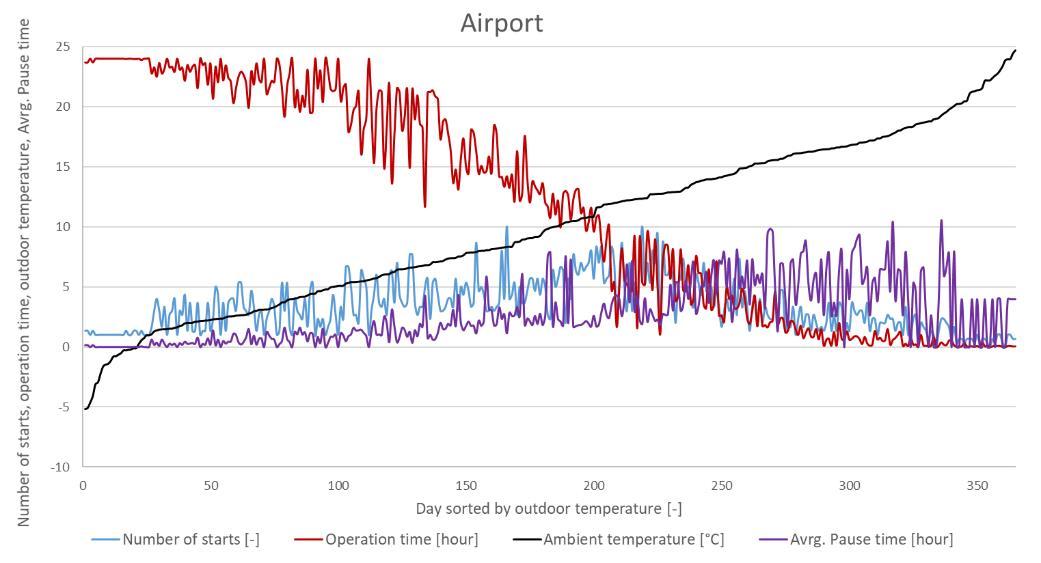
The overall performanceof the systemis given in Figure 1.1-5, where weeklyperformance indicators are plotted. At low outdoor temperaturesthe operationtime isalmostall day,meaning the heat pump is running continuously. When the outdoor temperature increases, the operation time decreases allowing for longer periodswithoutheat pump operation.
8
Figure 1.1-4 System COP for the heat pump installed at the airport.
Figure 1.1-5 Performance of the systeminstalled at the airport.
1.2 Added control system installed in the airport
The Bosch heat pump runs onitsinternal control strategybut in thisproject three relays are designed and implemented for external control purpose.If relay1 is activated theheat pump is shut off.If relay2 is activated the pump supplying the airportwith heat isshut off. If relay 3 is activated the heat pump isturned on for force running of the heat pump lifting the heating profile controlling the heat pump.
The APIcontrol programwas setup remotelycontrolling Relay 1 and Relay 2 according to the indoor and outdoor environment.
First, it will connect Neogrid Gateway and askfor the real time data of the indoor and outdoor temperatures.Second,bycomparing the indoor and outdoor temperatureswith the threshold temperatures,the control signalsfor Relay 1 and 2 will be calculated according to the control strategy. Then the control signalswill be sentoutto the Neogrid Gatewayand implement the control signals to the Relays. The control start time,stop time and the time step can be specified byusers. The APIcontrol is deployed in the DTU server and runscontinuously24 hoursper day.
Reduce run time for the heat pump when the outdoor temperature is high
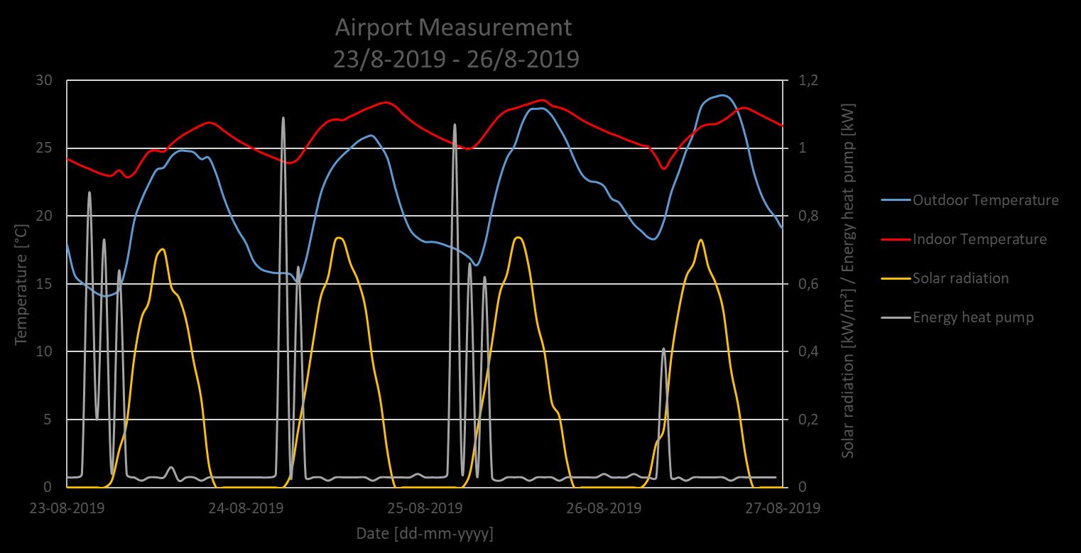
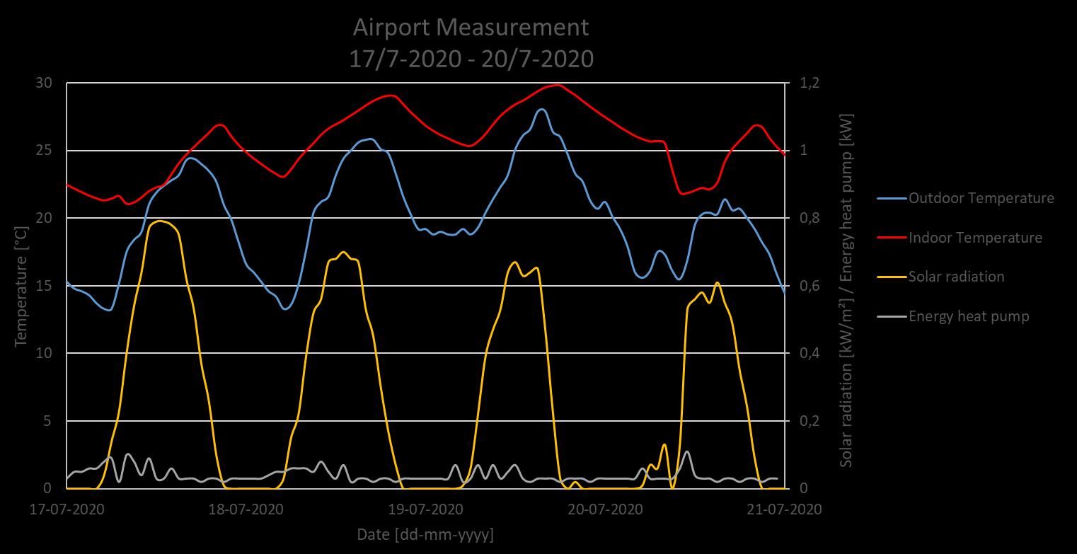
It was observed that the heat pump would startup during periodswhere there was no need for heating since the indoor temperature was well above 20°C. This isbecause the heat pump doesnot look to the indoor temperature,butis controlled bya profile based on the outdoor temperature as well as other internal algorithmswhere time playsa role.The unneeded starting of the heatpump can be seen on Figure 1.2-1 where the red curve is the indoor temperature and the grey curve isthe energy consumption ofthe heat pump.The blue curveis the outdoor temperature and the yellow curve is the solar radiation,which shows these days were sunnydayswith high temperatures during the day.
The added control implemented the1st of July 2020,simplystatesthatif the indoor temperature is above 20°C, relay1 is pulled and the heat pump isblocked from starting.When the indoor temperature dropsbelow 19°C the blockis lifted and relay1 is released meaning the heat pump is
9
Figure 1.2-1 The in- and outdoor temperature as well as the solar radiation and energy consumed by the heat pump from the 23/8-2019 to 26/8-2019.
returned to itsnormal controls. The effect of this can be seen on Figure 1.2-2 where the energy consumed bythe heat pump isreduce to a minimum, which is needed for running the control system internally in the heat pump.
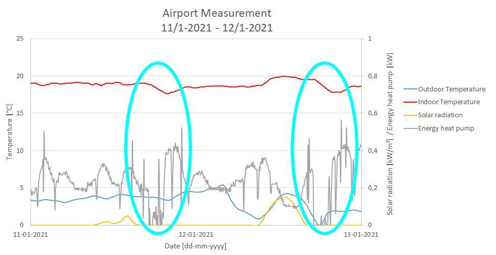
Reducing the energy consumption during peak hours in the winter period. To utilize the flexibility the storage tank offersadditionalcontrols were implemented. The control states that the heatpump shutsdown at hour 17:00 to hour 20:00. If the room temperature drop below 17°C the heat pump is released and returned to its normalcontrol.
10
Figure 1.2-2 The in- and outdoor temperature as well as the solar radiation and energy consumed by the heat pump from the 17/7-2020 to 20/7-2020.
Figure 1.2-3 The in- and outdoor temperature as well as the solar radiation and energy consumed by the heat pump from the 11/1-2021 to 13/1-2021.
The effectsof the added controlscan be seen in Figure 1.2-3.The two circlesshow the time periods where the heat pump is forced to shutdown.The grey curvesindicate theenergyconsumption ofthe heat pump, and show it is lowered in thistime period. The red curveshowsthe indoor temperature and here the effectsof the forced shut down on the indoor temperature. It can also be observed that there is a delay in the drop in indoor temperature, which isthe effectsof the storage tank. The storage tankcontinuesto deliver energy to the building after the heat pump isshutdown.When the tank temperature is below the roomtemperature the building is no longer supplied with heat and therefore the indoor temperature drops.When the lower limitof 17°C is reached theheat pump is released and the consumptionof the heat pump shows itturns on and startssupplying the building with heat again.
On Figure 1.2-4 the effecton the system COPbefore and after the control were added are given. Here it can be seen that the added control hasa positive effect on the systemCOP.During the summer months unnecessaryrun-time is reduced. During the winter monthsthe systemCOP is increased.
Experiences running the heat pump through relays and API controls
In order to maintain a robustcontrolsystem, the APIcontrolis further designed with the following extra functions.
1. Automatic fallbackcontrolsignal.When a signal iscalculated and sentoutto the relay,the signal alwayscontainstwo parts.The first part isthe currentcontrolsignal and then followed by a 0 signal for the nexttime step. This isto make sure thatonce the control collapsesor fails, the relaycan fall backto itsinitial condition.
2. Automatic notification.The controlsystemcan automaticallysend emails to notifyusers that the controlstarts, stopsand errors found.
3. Hold on period. It appears thatsometimesthe Bosch systemare offline due to WIFI problems. Then the control system cannot request the real time data fromNeogrid Gateway. Then the controlsystemcan hold on for a period that user specified and attempt to connect again. The total attempttimes before error reporting can also be specified.
4. Control file.The control systemcan automaticallyrecord all the control signals, control status and time stepsand writeto a log file with the name of thestartdate.
11
Figure 1.2-4 The system COP before and after the controls are added to the system.
2. Systemdescriptionprivatedwellings
2.1
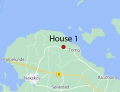
House 1 is a brickhouse builtin 1947, located in Lolland,see Figure 2.1-1.The occupantsare a family with three adultsand one child.The space heating loop consists ofradiators with a forward and return temperature of 55°C and 45°C.
The house was previously heated byan oil burner,with a yearlyconsumption of 2000 liters.In September of 2019 the house wasfitted with a new system fromSuntherm,consisting of a 7kW heat pump and a 400 literswater and PCM storage.Keyfiguresfor House 1 and the system installed is given in Figure 2.1-1 The measurements used in the analysisare from 1st of November 2019 to the 1st of June 2021.

* the building heat loss is determined based on measurements of the delivered space heating during periods with a constant indoor temperature.
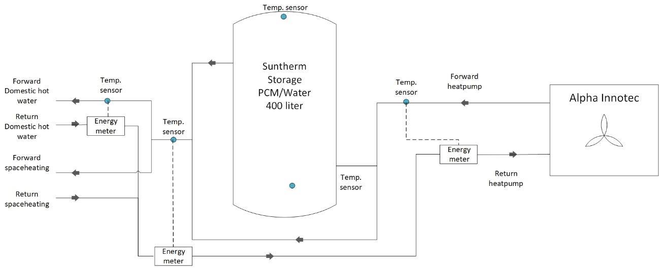
A sketch of the system installed is shown on Figure 2.1-2 The systemisdesign to cover both space heating and domestichot water.On the figure,the heat pump isshown to the rightwith connections
12
House 1
Figure 2.1-1 Location of House 1 and a picture of the house.
House 1 Building area 125 [m²] Year of build 1947 [-] Building heat loss* 0.265 [kW/K] Building time constant 57 [hour] Building heat capacity 15 [kWh/K] Size heat pump 7 [kW] Size buffer storage (water/PCM) 400 [liters] Measurements from 1/11-2019 [dd/mm-yyyy]
Table 2.1-1 Key figures for House 1 and the system installed.
to the storage in the middle.The systemis designed with a by-passoption so theheat pump can deliver directlyto the house. The additional energymetersinstalled in the systemare also shown in the figure.
Space heating
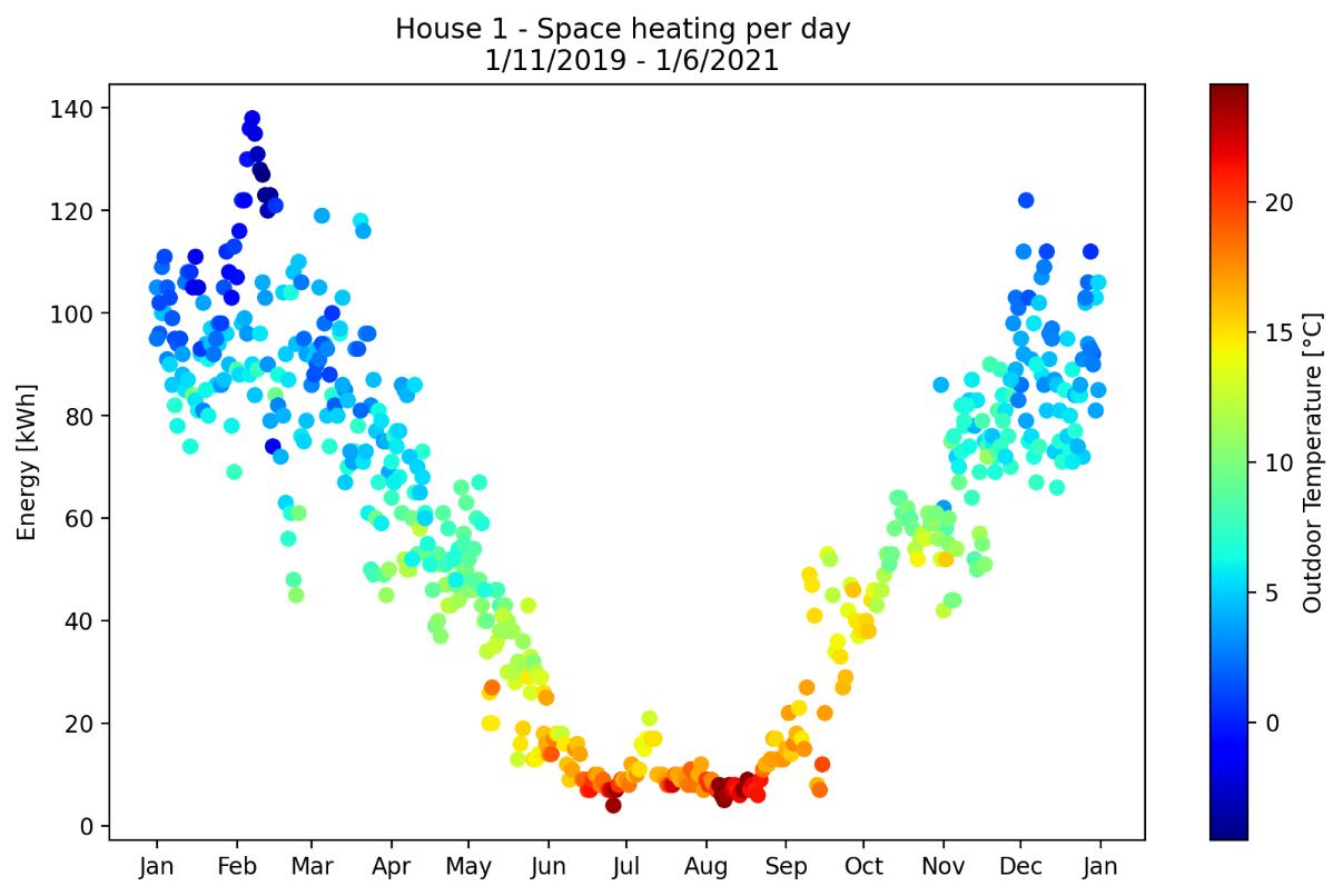
Based on the collected measurements theenergyused for space heating is determined and given in Table 2.1-2. The energy consumption for space heating is of course dependentonthe weather conditionsduring the heating season For house 1 the space heating need is approx.20 MWh per year.
The daily space heating need is also shown on Figure 2.1-3 over the course of a year The mean daily outdoor temperature is indicated with colour corresponding to the outdoor temperature,see scale to the right. When the outdoor temperature increasesthe energyfor space heating decreases and comesclose to 0 kWh atoutdoor temperaturesof 17°C.
13
Figure 2.1-2 Sketch of the systeminstalled in House 1 delivered by Suntherm.
House 1 – Space heating 2019 2020 2021 1/11 – 31/12 1/1 – 31/12 1/1 – 1/6 Degree days [-] 692 2370 1764 Energy Space heating [MWh] 4.96 19.68 11.30
Table 2.1-2 Energy for space heating House 1 from the 1/11-2019 to 1/6-2021.
Domestic hot water
The same way the energy for space heating is measured so is the energyfor domestichot water. The family hasyearlyenergyconsumption of approx.1.0-1.5 MWh, see Table 2.1-3 Also, their daily consumption isbetween 119 litersand 151 liters.
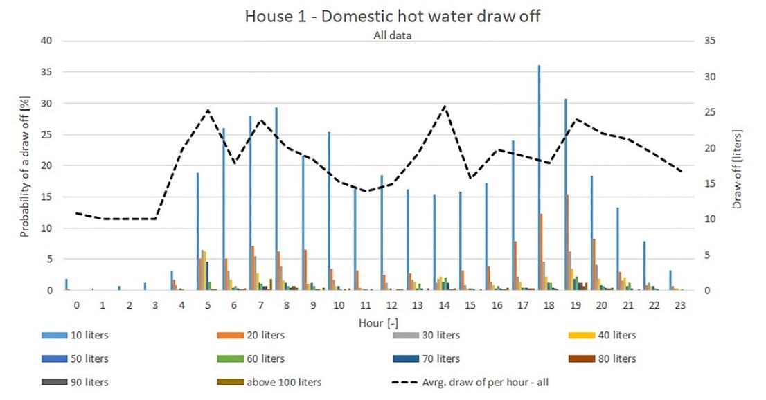
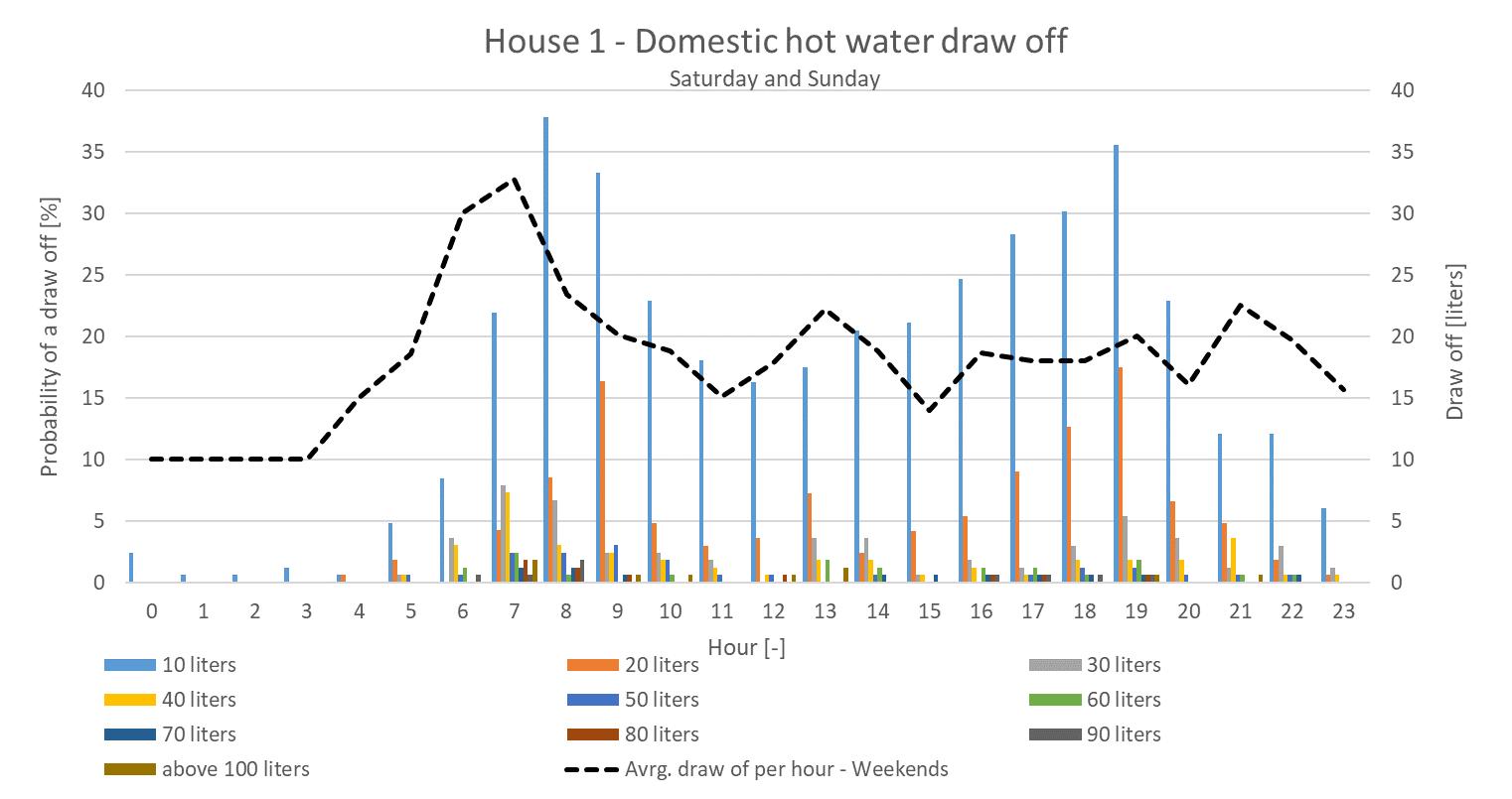
The measurement also givesinformation of the pattern for the domestichotwater draw off. On Figure 2.1-4 the average draw off over the courseof 24 hoursis given, along with the probabilityof differentsizesdraw offbased on all the measurements.
14
Figure 2.1-3 The need for space heating for house 1 as a function of the time of the year, with the colour indicating the outdoor temperature.
House 1 – Domestic hot water 2019 2020 2021 1/11 – 31/12 1/1 – 31/12 1/1 – 1/6 Energy domestic hot water [MWh] 0.28 0.93 0.95 Average draw off per day [liters] 119 127 151
Table 2.1-3 Energy for domestic hot water for House 1 from the 1/11-2019 to 1/6-2021.
The vertical barsgive the probabilityof a certain size hot water draw off within a specifichour, excluding the hourswhere there are no draw off. The blue barsindicate a 10 liter draw offand therefore is the most common draw offin all the hours. This givesan indication of when there are large hot water draw off and if there are hourswhere it is unlikely there are hotwater draw off. Larger draw off are seen in the morning hoursand dinner time hours. The average draw offper hour show on the figure withthe dotted curve givesthe average size of the hot water draw offonlytake during periods with draw off. Here it isseen thatthere are large hot water draw offsduring the morning hoursfrom 5 to 8 am and again at 2 pm.In evening there are again large draw offsaround 7 to 8 pm.
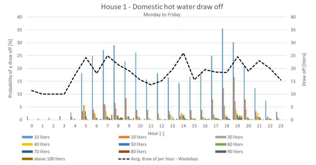
Based on the measurementscollected itis also investigated if there are differentprofilesfor the differentdaysof the week. For House 1 the profilesfor weekdaysand weekendsare much the same, which can be seen on Figure 2.1-5 and Figure 2.1-6
15
Figure 2.1-4 Probability of a draw off from House 1 and the average draw off based on all data.
Figure 2.1-5 Probability of a draw off from House 1 and the average draw off based on data from Monday to Friday.
On weekdaysthere are lesslarge draw offsin the evening compared with the weekends,at the same time there is a higher probabilityof a 10 liters draw off during the nightin the weekdaysas oppose to the weekends.
Performance
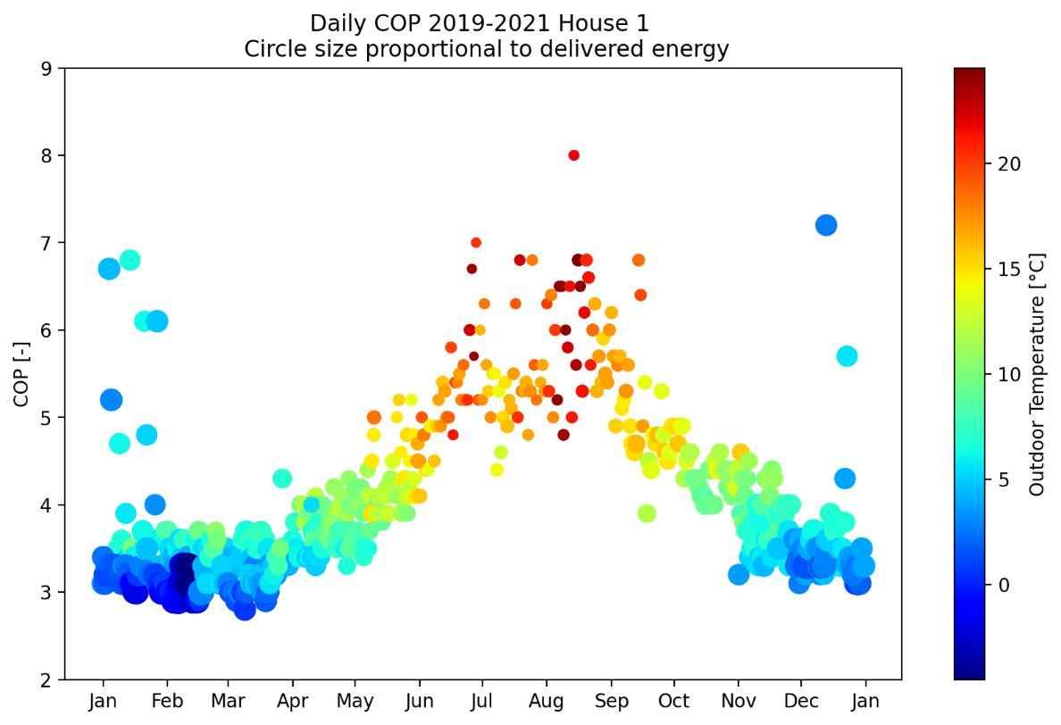
The efficiencyof the systeminstallationin House 1 is given on Figure 2.1-8 The SystemCOP is shown over the course of a year where the outdoor temperature isindicated with the colours. The sizes of the circlescorrespond to the energy delivered to the house by the heatpump.
16
Figure 2.1-6 Probability of a draw off from House 1 and the average draw off based on data from Saturday and Sunday.
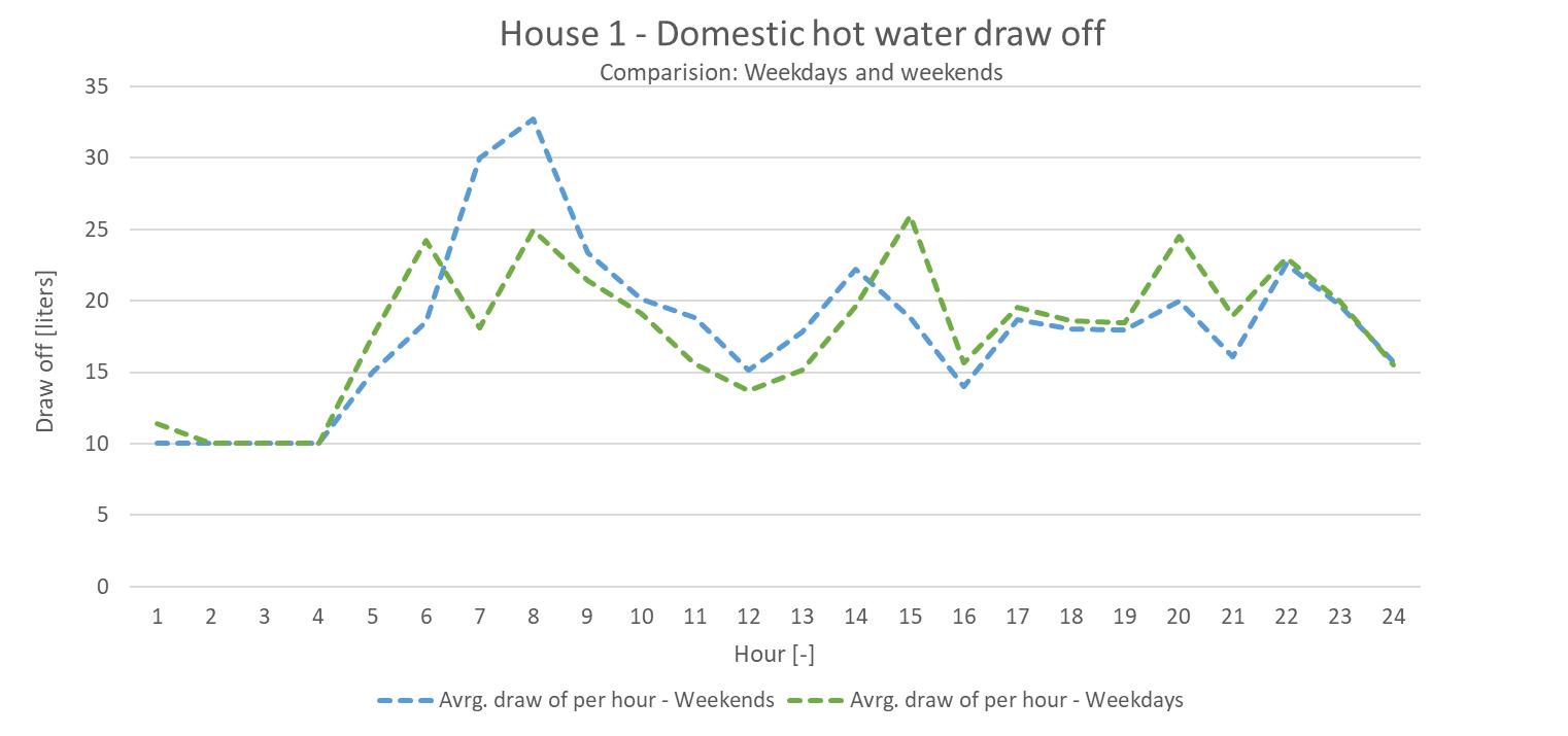
Figure 2.1-7 showsthe difference in the weekdaysand weekend profiles, where it becomes clearer that there is a higher probabilityfor larger draw offsduring the morning in the weekends.
Figure 2.1-7 Comparison between weekdays and weekend profiles for House 1.
The System COPis between3 – 7, which is considered asa well operating heat pump. The System COP is temperature dependentas itis seenon the figure, with higher performance atwarmer outdoor temperatures.
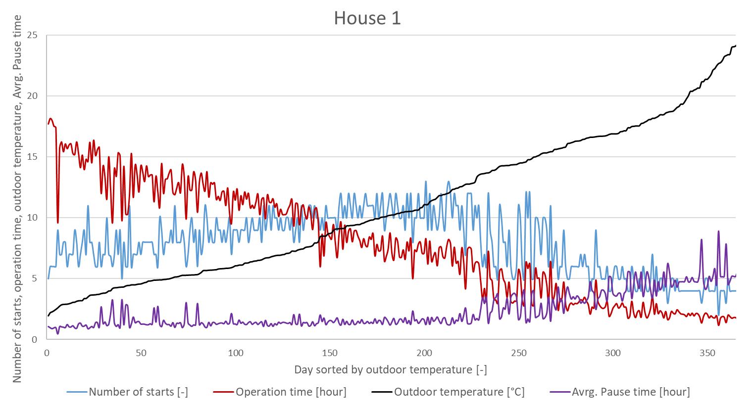
On Figure 2.1-9 the overall performance of the Sunthem system isgiven. Here it can be seen that the operation time at low outdoor temperaturesis approx. 16 hours,with avg.pause time around 1-2 hours. At increasing outdoor temperatures, the operation timedecreases and the avg. pause time increases. This indicatesthatthere is a potential for flexibility.
17
Figure 2.1-8 System COP for the heat pump system installed at House 1
Figure 2.1-9 Performance of the systeminstalled at House 1.
2.2 House 2
House 2 is located in the southern part of Zealand on Bogø, see Figure 2.2-1. It is a wood house build in 2005. Two adultswith one child occupiesthe house.The previousenergy source before the installation of the Sunthermsystem waselectricitywith a yearly consumption was 19.000 kWh.


Radiatorsheat the ground floor of the house and the firstfloor is heated byfloor heating.
Key figures for the house and systeminstalled for House 2 is given inTable 2.2-1
The heat pump installed is a 7 kW heat pump with a 400 literswater and PCM storage.The measurements are available from1st of December 2019.
* the building heat loss is determined based on measurements of the delivered space heating during periods with a constant indoor temperature.
18
Figure 2.2-1 Location of House 2 and a picture of the house.
House 2 Building area 179 [m²] Year of build 2005 [-] Building heat loss* 0.170 [kW/K] Building time constant 84 [hour] Building heat capacity 14.32 [kWh/K] Size heat pump 6 [kW] Size buffer storage (water/PCM) 400 [liters] Measurements from 1/12-2019 [dd/mm-yyyy]
Table 2.2-1 Descriptive figures for House 2 and the systeminstalled.
Space heating
Table 2.2-2 shows the measured energy for space heating in House 2 along with the number of degree days.The yearly energyconsumption for space heating isapprox.10 MWh per year.
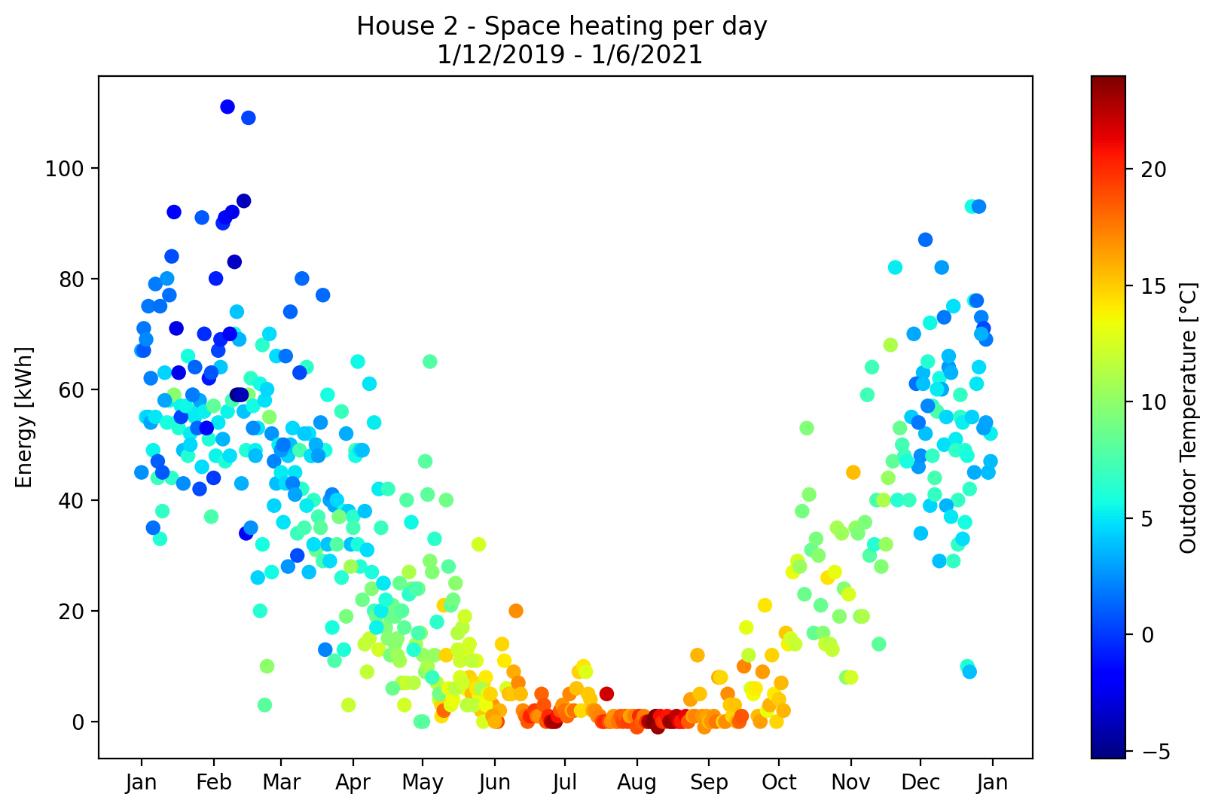
The energy for space heating over the course of a year is shown in Figure 2.2-2. The dependencyof the outdoor temperature can be seen with the colour scale indicating the variation of the outdoor temperature. It can also be seen that House 2 has a much lower heat demand for space heating compared to House 1, which is because thehouse is more recently build with more insulation according to the harder restrictionsin the Danish build code.
The energy for domestichot water usage for House 2 is approx. 1.4 MWh per year,with an average daily consumption of just under 100 liters per day,see Table 2.2-3
19
House 2 – Space heating 2019 2020 2021 1/12 – 31/12 1/1 – 31/12 1/1 – 1/6 Degree days [-] 377 2368 1788 Energy Space heating [MWh] 1.74 9.52 6.16
Table 2.2-2 Energy for space heating House 2 from the 1/12-2019 to 1/6-2021.
Figure 2.2-2 The need for space heating for house 2 as a function of the time of the year, with the colour indicating the outdoor temperature.
The profile of the domestichotwater consumption in House 2 can be seen on Figure 2.2-3 based on all the data available fromHouse 2. The figure shows a high draw offin the early morning hours. Also in the morning,occurrence of smalltapsof 10 liters isalmostno existing.The figuresshow most often the tapsin the morning are larger ranging from 30 liters to 50 liters.
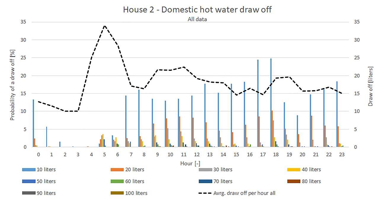
The evening peakwhere larger tap occurscan beseen from hour 18 to hour 19,
taps
30 liters and more.
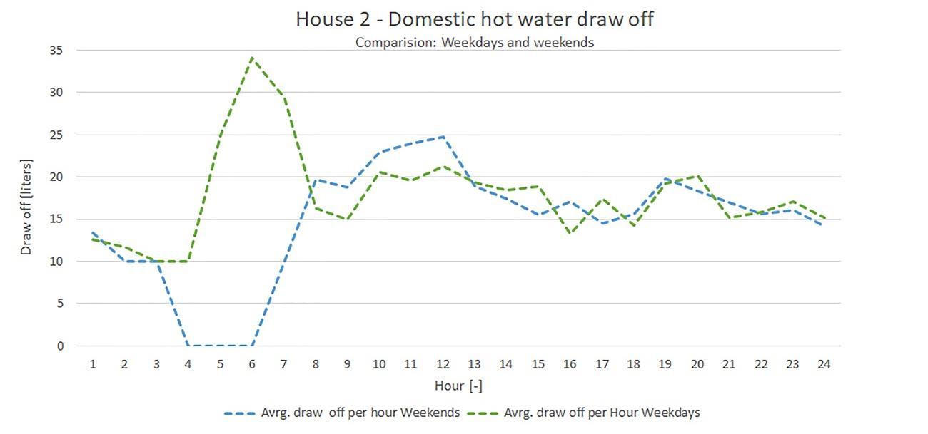
When the data is spilt into weekdaysand weekendsand profilesare created it appear that the early morning draw offdoes not occur in the weekends, seeFigure 2.2-4 The consumption of hot water is moved fromthe earlymorning hours at 5-6 in the weekdaysto the hours of 8-12 which isseen with the increase in the average usages in the profile for the weekend (blue curve).
20
House 2 – Domestic
2019 2020 2021 1/12 – 31/12 1/1 – 31/12 1/1 – 1/6 Energy domestic hot water [MWh] 0.12 1.39 0.61 Average Tap per day [liters] 95 98 90
Table 2.2-3 Energy for domestic hot water for House 2 from the 1/12-2019 to 1/6-2021.
hot water
Figure 2.2-3 Probability of a draw off from House 2 and the average draw off based on all data.
with
of
Performance
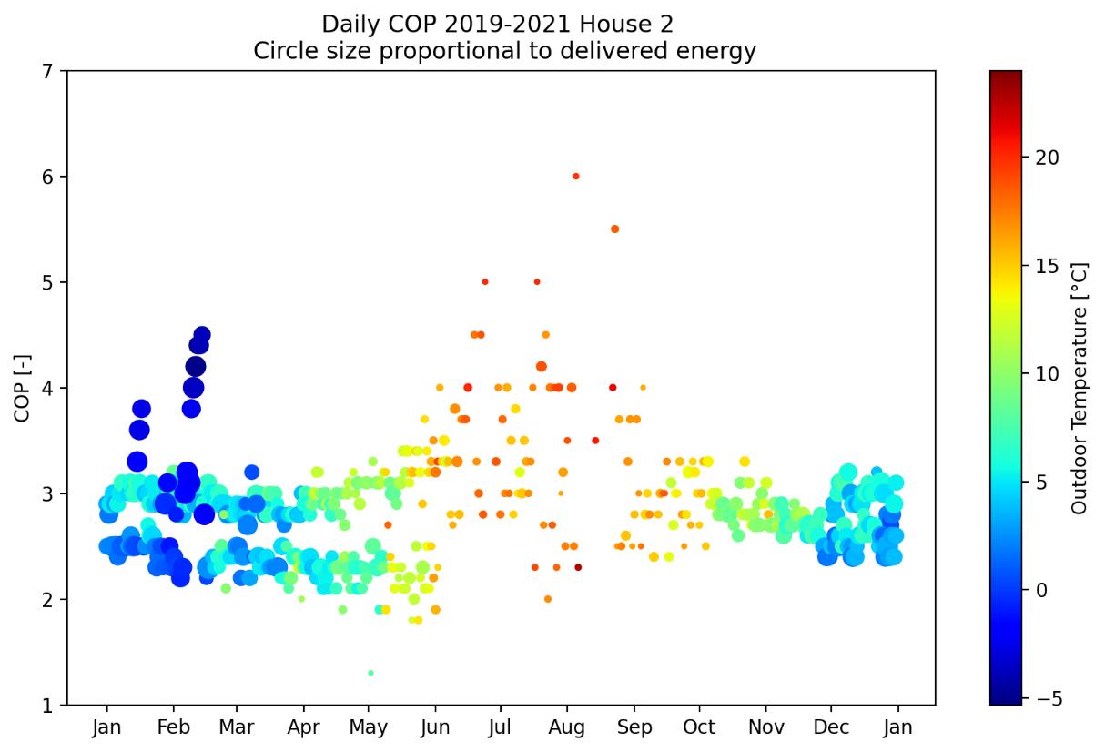
The system COPfor the Suntherm system installed at House 2 is given in Figure 2.2-5,where it can be seen that the system COPis between 2.0 and 5.0 dependentonthe outdoor temperature. In the figure, the size of the circlescorrespondsto the delivered energyby the heat pump to the house. It can be seen that as expected the most energyis delivered during the winter monthswhere the space heating needsare highest.
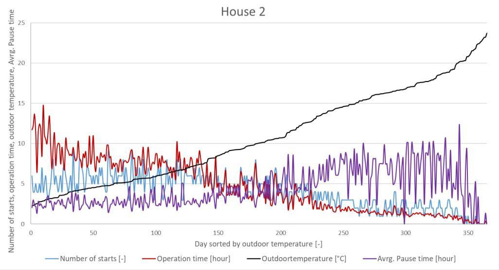
The overall performanceof the systeminstalled in House 2 is given in Figure 2.2-6.Compared with the systeminstalled in House 1,it can be seen thatthe operation time islowered, also there is an increase in the duration of the periodswithoutheat pump operation which meansthatthere is a
21
Figure 2.2-4 Comparison between weekdays and weekend profiles for House 2.
Figure 2.2-5 System COP for the heat pump system installed at House 2
greater potentialfor offering flexibility. The measurementsshow that the average duration of the periodswithoutheat pump operation reaches5-6 hourswhen the outdoor temperature is above 10°C. At outdoor temperatures around 0°C the daily operation time is approx. 13 hoursand the average duration of periodswithoutheat pump operation is 3 hours.
The houseis a brick house from1997 with 190 m² living area. It is heated with floor heating. It is occupied with two adults and one child. The house is differentfrom the other two houses, in regardsto the domestichot water. The house has a circulation pipefor the domestichot water ensuring hotwater as soon as the hot tap is turned on.
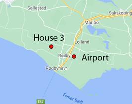
House 3 located close to the airport in the southern part of Lolland,see Figure

The previousenergysystemfor the housewas an oil burner with a yearlyconsumption of 1800 liters oil. The systeminstalled in this house is again a Suntherm system witha slightly bigger heat pump of 9 kW and a 400 liters storage tank with water and PCM.The configuration ofthe systemis the same as House 1 and House 2. The measurementsare available from1/12-2019.
22
Figure 2.2-6 Performance of the systeminstalled at House 2
2.3 House 3
2.3-1.
Figure 2.3-1 Location of House 3 and a picture of the house.
In Table 2.3-1 key figures for House 3 are given.
* the building heat loss is determined based on measurements of the delivered space heating during periods with a constant indoor temperature.
Space heating
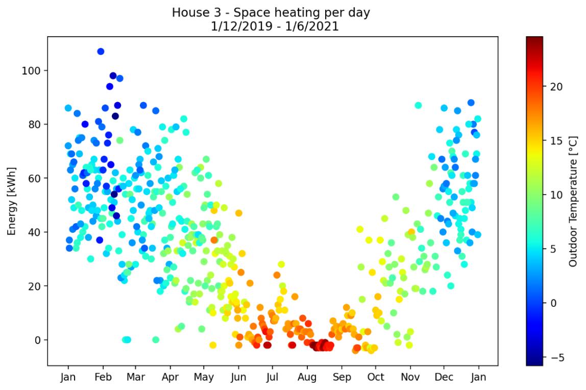
The yearly consumption for space heating is approx. 11 MWh,see Table 2.3-2, whichis much like the consumption for House 2. The consumption correspondswith when the house is builtand demand for insulation resulting in a low heat looscoefficientfor the house.
The space heating delivered to House 3 isshown onFigure 2.3-2 over the course of a year. Again, the outdoor temperature is given with the colour scale,where the higher consumption of space heating occurswhen the outdoor temperature is low.
23
House 3 Building area 190 [m²] Year of build 1997 [-] Building heat loss* 0.157 [kW/K] Building time constant 146 [hour] Building heat capacity 22.8 [kWh/K] Size heat pump 9 [kW] Size buffer storage (water/PCM) 400 [liters] Measurements from 1/12-2019 [dd/mm-yyyy]
Table 2.3-1 Key figures for House 3 and the system installed.
House 3 – Space heating 2019 2020 2021 1/12 – 31/12 1/1 – 31/12 1/1 – 1/6 Degree days [-] 376 2372 1777 Energy Space heating [MWh] 1.79 10.39 7.68
Table 2.3-2 Energy for space heating House 3 from the 1/12-2019 to 1/6-2021.
Domestic hot water
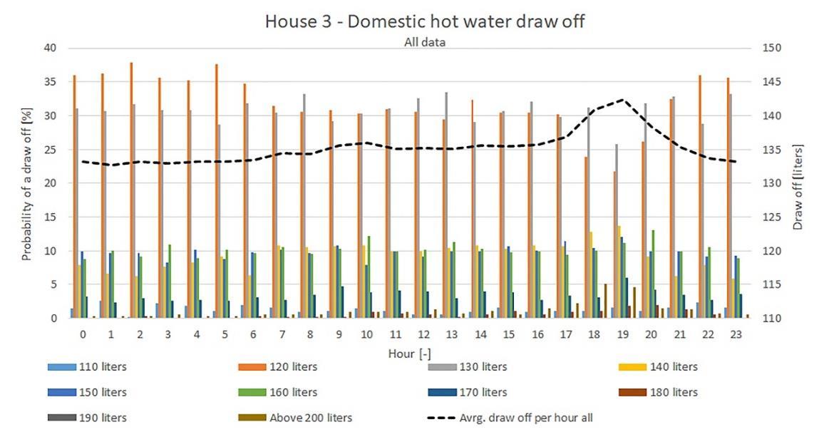
There is, as mentioned earlier, a circulation pipe for the domestic hotwater, which appear in the yearly consumption measured in the house of approx.10 MWh, see Table 2.3-3 The consumption here consists of the lossesfrom the pipesand the domestic hotwater consumption.Also because of the circulation the dailyconsumption ofhotwater in litersis not given, butthe litersflowing through the energy meter incl.the circulation.
On Figure 2.3-3 the average hourly consumption isshown with the blackdotted curved. Because of the circulation it isdifficult to detectan actualprofile,only an evening peakaround hour 17 to 20 can be seen.
24
Figure 2.3-2 The need for space heating for house 3 as a function of the time of the year, with the colour indicating the outdoor temperature.
House 3 – Domestic hot water 2019 2020 2021 1/12 – 31/12 1/1 – 31/12 1/1 – 1/6 Energy domestic hot water [MWh] 0.86 9.47 4.16 Average flow through the energy meter per day [liters] 3580 4149 2987
Table 2.3-3 Energy for domestic hot water for House 3 from the 1/12-2019 to 1/6-2021.
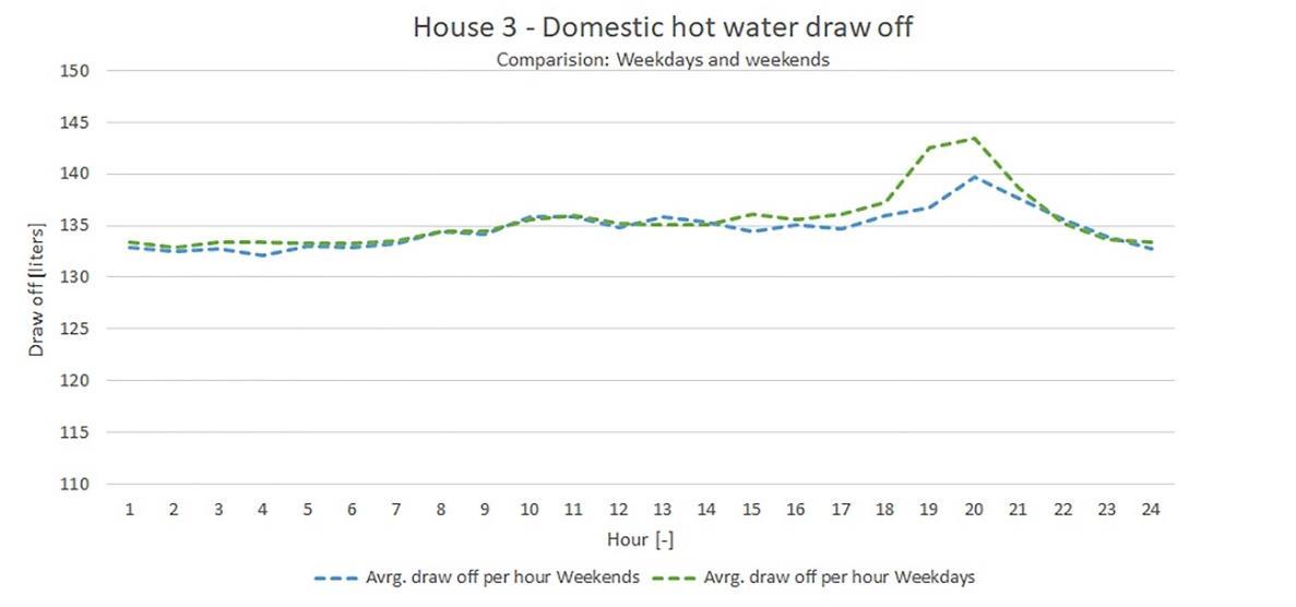
The same difficultiesto detect profiles isalso seen in Figure 2.3-4 where weekdayprofile is compared with weekend profile.
Performance
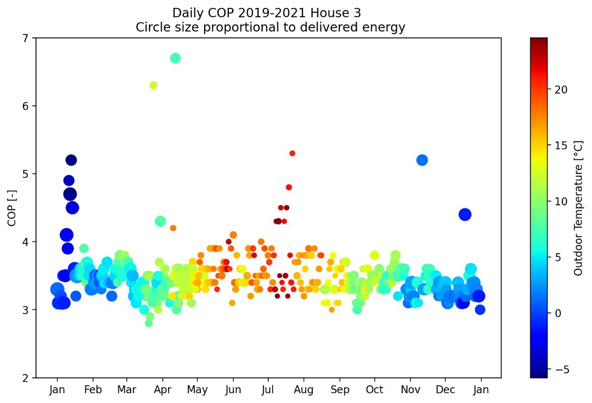
The system performance of House 3 is shown on Figure 2 3 5. Here it can be seen thatthe daily system COPis more or lessconstant around 3.5.
25
Figure 2.3-3 The effects of circulation on the probability for House 3 and the average draw off based on all data.
Figure 2.3-4 Comparison between weekdays and weekend profiles for House 3.
The size of the circlescorresponds to the amount ofenergydelivered bythe heat pump. Because of the circulation on the domestichot water,the operation of the heat pump ishigher during the summer months compared with the other two-familyhouses.
The overall performancefor the systeminstalled in House 3 is given in Figure 2.3-6.On the figure it can be seen the average duration of periods without heatpump operation and the number of starts is more or less constantover the course of a year. The operation time over the course of a dayranges from 13 hoursto 2 hours.
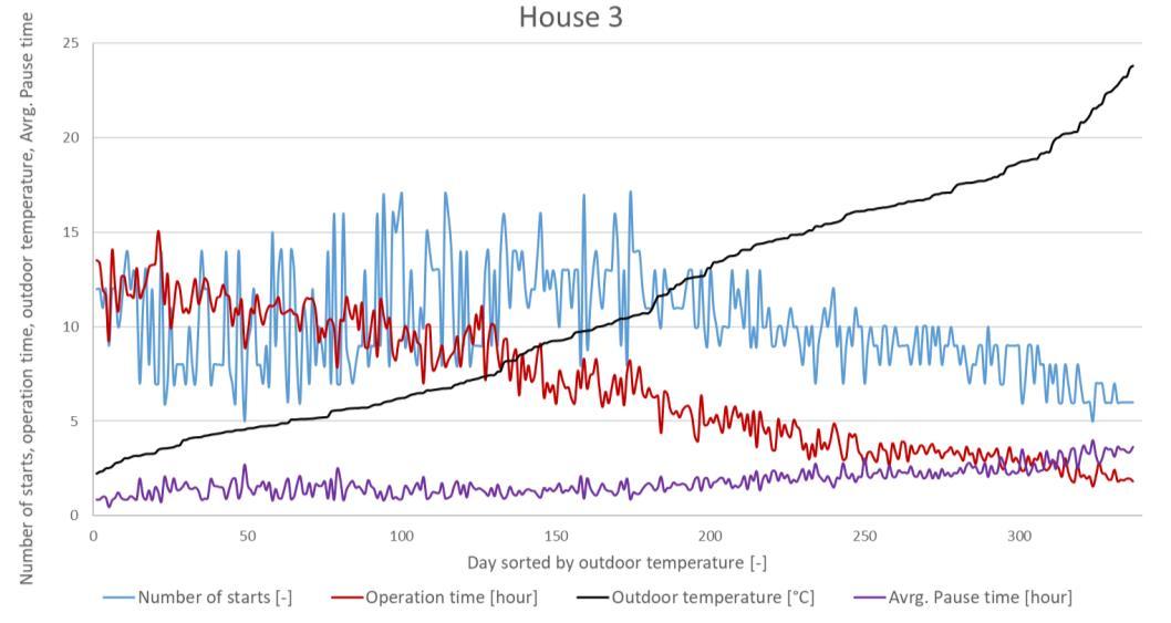
26
Figure 2.3-5 System COP for the heat pump system installed at House 3.
Figure 2.3-6 Performance of the systeminstalled at House 3.
3. Storagecapacityandpotential
Thermal energy storage isan importantcomponentin energysystems,especially when there is a wish to shiftbetween when energyis produced and when energy isused.Having an energy storage will allow for an increasein utilization of sustainable energy.
Three typical typesof storage for energy system are: Sensible heat storage, heatof fusion storage and chemical storage. A sensible heat storage is utilizing a temperature increase in a heat storage material, usuallywater. Heat of fusion storage iswhere a phase change is utilized in order to increase the energy contentper volume compared with e.g. water.In chemical storage a chemical reaction is utilized in the storage.The chemical storagesare not included in thisproject,and are therefore not described further
3.1 Water storage
Water storagesare the most common sensible heat storage and are usually cylindrical tanksmade of steelor stainlesssteel with water inside.The freezing point for water is0°C and the boiling pointis 100°C, making the operating temperature vary from0°C to 100°C, which correspondswell with demands for many energysystems.
For the Bosch system installed in the airportthe operating temperature of the storage is between 30°C to 45°C with a water volume of 300 liters. The theoretical energy contentin the storage is 5.2 kWh. The measured discharge power fromthe storage is between1.5-2.0 kW. The total energy discharged from thetank during a shutdown period is approx.4.5-5 kWh over the course of 2-2.5 hours.
3.2 PCM storage
In a phase change storage, a large partof the heat isstored during the phase change ofthe heat storage material.The most promising change isfrom solid to liquid phase since many materialshave a melting pointbetween 25°C to 70°C, see Table 3.2-1
The PCM material used bySuntherm hasa melting pointof 48°C. A comparison between the theoretical heatcontent of 100 l storeswith water,PCMwith a melting point of 48°C and PCM witha melting point of 58°C is given in Figure 3.2-1
27
Formula Melting point, °C Heat of fusion, kJ/kg salthydrate Sodiumcarbonate decahydrate Na2CO3∙10H2O 33 247 Sodiumthiosultfate pentahydrate Na2S2CO3∙5H2O 48 209 Sodiumacetate trihydrate NaCH3COO∙3H2O 58 265
Table 3.2-1 Different salt hydrates which can be used as heat storage material.
The blue curve shows the heat content in a 100 liters volume of PCMwith a melting point of 48°C. Up until the melting point the increase in energymore or lessfollowsthe increase in the 100 liters water volume. When the melting pointis reached, the temperature remainsat 48°C while the heat content increasesand the PCMchangesfrom solid to liquid. When all PCMis melted,the temperature increases again during charge of the heat storage. The orange curve showsthe same pattern for a PCM with a melting pointof 58°C. The dotted curve shows heat contentof the water storage.
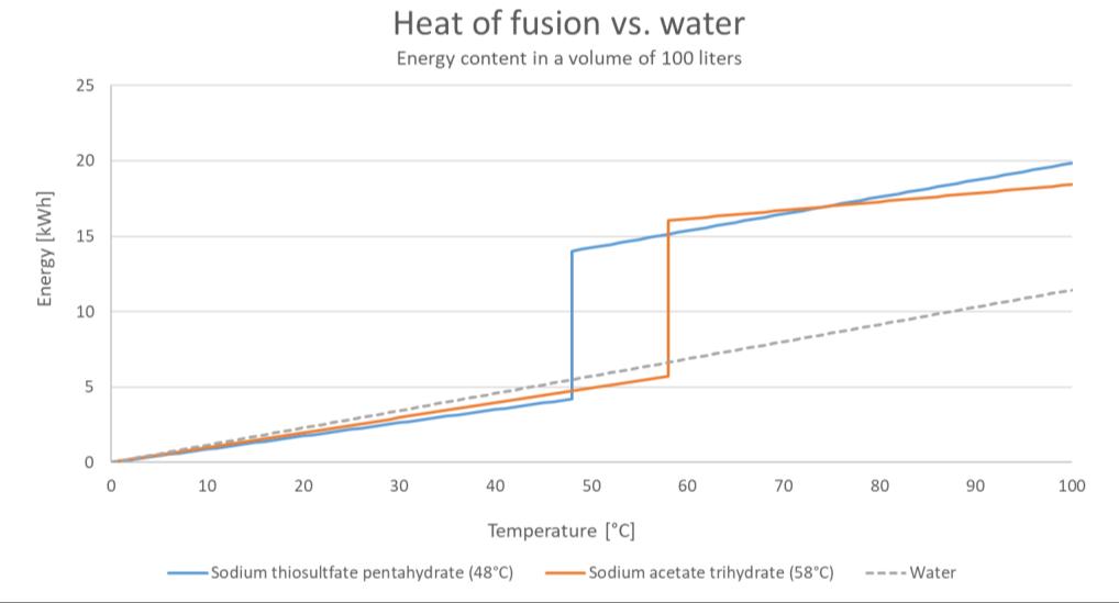
Overall, it can be observed thatthere isa great potential in utilizing the latent heat contentin the PCM compared with sensible heat contentin water. The PCM allowsfor larger heat storage capacities without increasing the volume.
The Suntherm storages installed in thisprojectall have a volume of 400 liters.Of the 400 liters30 % is PCM material, 66 % iswater and 4 % isthe plasticencapsulating the PCM. The operating temperatures in the storages are from47°C to 58°C.
The maximum theoreticalheat content in the Sunthermstorages is 11.4 kWh,where the water accountsfor 3.6 kWh and the PCM for 7.8 kWh. A water storage with a heat contentof 11.4 kWh in the same temperature interval 47°C-58°C would have a volume of 893 l. That is, the water storage volume would be 2.2 timeslarger than the PCMheat storage used by Suntherm.
In this project, the measured discharge power fromthe Suntherm storagesis approx.2.5 kW depending on the control settingsin the storage tank. In total the energydischarge from thetank during a shutdown period is between 4.0– 5.0 kWh of the course of 1.5 – 2 hours.
One of the obstacles making it difficult to utilize more of the energyin the PCM isthe plastic encapsulating the PCM. It hinders a high heat transfer fromthe PCMto the water and vice versa. Also, the theoretical energycontent calculated for the PCM isbased on verysmall quantities determined byT-historymethod. Investigationshave shown difficultiesin upscaling the volumeof PCM and obtaining the same latentheat content because of phase separation problemsin the PCM.
28
Figure3.2-1 Heat contentof100 l stores with water and PCMs
4. Optimisedcontrolofheatpumps
4.1 Introduction
Some of the heat pumpsin the FUTURE projecthas been connected to Neogrid server and optimised controlhas been applied. In thischapter the optimised controlis explained and the results from the analysisand tests are shown.
4.2 Heat pump survey and control access
Heat pumpscan be separated into 3 categories with regard to their “Smart Grid Readiness”.
In order to make a heat pump useful for optimised control basicdata must be logged and sent to Neogrid’sserver.Then analysistake place and an operation schedule for the heat pump is calculated and sent back to the heat pump.This can be implemented in differentwaysdependant on the type of heat pump.
● Gateway with relay control
1 Standard heat pump with relay input
2 Bigger heat pumpsand heat pumps with Modbus(RS-485) interface
3 Cloud connected heat pump with APIfor logging of data and control
● Room temperature sensor
● PT-1000 outdoor temperature sensor emulator
● Gateway with RS-485 interface
● Room temperature sensor
● Nothing
The table above shows three typesof heat pumps and the required retrofit in order to make the heat pump ideal for optimised control. Older and/or simpler heat pumps(cat1) requires a gatewayto get it online and to collectall sensor and meter data.Control isestablished via theheat pumpsrelay input or bymanipulating the outdoor temperature sensor. Other heat pumps(cat 2) have a communication interfacewhere much more data and control capabilitiesare available.Newer heat pumps (cat.3) are “born” online and have the possibilityto collectdata from external sensors and meters. The heat pump manufacture typicallyoperatesa cloud where all data are collected and available for a third-party actor like Neogrid via an API.
Heat pumpsused by Sunthermin the FUTURE project belong to cat 3,with full onlineaccessto all data and control setup.The Bosch heat pump in the airport iscat 1 type.
4.3 Flexibility
For a given installation the flexibility isthe heat pumpscapabilityto postpone or put forward its operation and still deliver the agreed comfort.Manyparameters in the installationdetermine the flexibility, some typical are listed in the tablebelow:
1 Energy and electricitymeterdata is assumed to be available
29
Table 4.2-1 Heat pump types and add-on equipmentfor optimized control Heat pump type Necessary equipment for optimized control1
Table
Parameters which determine flexibility
Big storage tank
Big domestic hotwater tank
Big heat pump
Frequencycontrolled heat pump vson/offtype
Ground water heat pump vsair water type
Large heat capacityof building
High time constant ofthe building
Low temperature for the heat pump
No limiting thermostatsinside building
Use of floor heating
Relaxed comfort requirementsinside building
Use of woodburner
Use of shortshowering
For a typical building a simple model to describe the dynamicsare:
where
• Pheat
Power delivered to the house [kW]
• Ti, Ta In- and outdoor temperature [˚C]
• Ri
• ksun
• C
• kbase
Heat resistance fromindoor to outdoor [˚C/kW]
Transfer function between out- and indoor sun power [1/m2]
Heat capacity of thehouse [kWh/˚C]
User behaviour generated power to the house [kW]
For “house 2” of the Suntherminstallations(the newer wooden house) the keyfigures: Ri, ksun,C and kbase are determined. It’salso tested thatone degree of variation on the indoor temperature is acceptableand then itis possible to determine the dailyamountof flexibilityin hours.This is plotted in Figure 4.3-2
30
4.3-1 Parameters determineflexibility
+ C Ta Ti Ri ksun · Psun Pheatkbase
Figure 4.3-1 Buildingmodel for astandard house
In the above figure daily key valueslike“No of starts”, “run time”, “rest time” and “1-degC flexibility” are sorted based on ascending Toutand plotted. “1-degC flexibility” is the duration it takes for the indoor temperature to drop one degree based on thespecific weather. It can beseen thatthishouse has minimum 5 hoursof flexibility even on the coldestday.This meansthatthishouse in bestcase can handle 5 hours with no added heatif the indoor temperature is at maximumcomfortalways and thus avoid operation on these hours.It should however be noticed thathotwater storage capabilities and demand also has an impacton the available flexibility.
4.4 Value proposition
Table 4.4-1 Heat
Type
servicelist
1 Operation optimisation and monitoring
2 Services against
● DSO
● ElectricityMarkets
3 Aggregator services
● ElectricityMarkets
Heat pump owner
Value proposition
● Online access to keydata from heatpump
● Low operation cost
● Improved comfort
● Lower energy bill
● Reduced CO2 footprint
In Table 4.4-1 the value propositionsfrom a heat pump running optimized control are separated into three categories.The first categoryare servicesavailable assoon as data iscollected fromthe heat
31
Figure4.3-2 Daily operation characteristics for aSuntherm operated buildingduringayear
pump
pump and connected meters. Then calculation of keyperformance indicators ispossible like daily COP and can be delivered bya companylike Neogrid or a third-partyactor. If external control is activated extra services like MPC2 control can secure a lower operation costof the heat pump.This category“only” requiresa bilateral agreementwith the heat pump owner and a cloud connected operator.
In category 2 variable prices, tariffsand servicesto the DSO are taken into account. Variable prices and tariffsare rolled out over most of Denmark,butDSOsflexibility demand to cope with bottlenecks is still limited in Denmark.
In category 3 specialized servicesto the electricitymarketsare delivered.This mightbe regulating power and frequency reserves. Those servicesrequire separate settlement of the electricityto the heat pump and an aggregator isrequired to pool a number of heat pumps.Settlementis a little more complicated asthisgoesvia the aggregator, who getspaid from the aggregated service delivered. How this is then shared between the differentactors might depend on several factorslike: flexibility size, numbers of activation etc.
4.5 Optimized control
There exist two main types of control:Price signal-based controlor direct control.With pricesignalbased control, a price signal isbroadcasted and some local AIdetermines a schedulefor the heat pump. This isuseful for Smart Home devices reacting on variable electricityprices etc.For this project direct cloud-based control is applied as the heat pump is a bigger device and full knowledge of the heat pumpsoperation isrequired to deliver some of thewanted services.The optimised control ismainly tested on the Suntherm installationsusing the block diagramshown below.
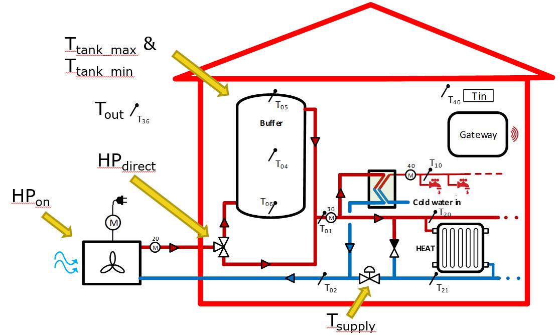
The main structure of the optimised control islike:
2 MPC – ModelPredictive Control, could be cloud based modeland weatherprognosis-based control
32
Figure4.5-1 Suntherm heat pump block diagramshowing controlinput
Table 4.5-1 Heat pump optimised controlalgorithm
Area
Details
● Variable net tariffs plan
● Variable electricitypricesplan
● CO2 content forecast
Inputs
Constraints
● Weather prognosis
● Heat pump COP vs Tout
● Heat pump COP v s Tsupply
● Heat pump defrosting demand vsTout
● Storage tanktemperature
● Heat pump run-/resttime
● Ti comfort window (maybe time dependent)
● Ttank max and Ttank min
● HPon
Output schedule: Control variable
● HPdirect heat pump delivering to tank or house
● Tsupply supply temperature for roomheating
The above table leasto the following mixed integer problemformulation:
n : nth timeslot
Tin : Indoor temperature [°C]
Tout : Outdoor temperature [°C]
Tset : Setpointindoor temperature[°C]
��,��,�� : Weightfactors
HPon : Heatpump on/off
Php : Electricity consumptionheatpump [W]
C : Cost function
COP : Heatpump COP
Pwater : Power domestic hotwater[W]
Pheat : Power roomheating [W]
Psun : Sun power vertical [W/m2]
Pmax : Max heatpump power [W]
Ttank : Temperaturein storagetank [°C]
dt : Time step size [h]
Vol : Storage tank volume [l]
c : Storage tank heatcapacity [Wh/°C/l]
��, �� : Matrices for state spacemodel
It should be noted in the problemformulation, thatthe solver iscapable ofhandling parameters,that are time varying.
33
���������������� ∑����(�������� ����������)+ +����(�������� ����������) �� ��=1 +���� ���������� ���� ������������������
������ ∈{0,1}(mixedinteger) ���������������� ≤������������ ≤ ���������������� ������=��(��������,��������������) ������������+1 =������������+ ���� ������∙��[���������� ��ℎ�� �������� �������������� ��ℎ��������] ��������+1 =���� ∙��������+����∙[���������� ���������� ��ℎ��������] ��������������������
����
4.6 Results and perspectives
Relay test on the Bosch heat pump atthe airporthas been carried out in the above sections.This section explainsthe optimized tests made on 3 Suntherm heat pump installations. Then the results are listed and discussed. The testshave mainly been carried outon 2 housesand not3 as one house owner decided not to join the tests.
First step in optimized control isto selectsome variable inputs. The analysishere are done with the variable DK1 spot prices3. Variable tariffsare included fromN1 a major DSO4,where peakhour prices are 0.54 dkk/kWh from 5 to 8 PM and 0.17 dkk/kWh outside thisperiod.
Second step is choosing a costfunction,in generalhere lowest price is selected.Other cost functionslike lowestenergy,minimumindoor temperature variation or lowest CO2 contentcould have been selected.
Third step is setting up constraints for the optimisation.This is mainlyaboutindoor comfort and domestichot water temperature.Indoor temperature variation on 1 °C in totalis selected as thiswas not really noticeable bythe participants. Tank temperature limits were setto 47 °C as low and 53/58 °C as high. Boosting tanktemperatures means higher capacityfor hotwater production but also a reduced COP.The low tank temperature still secured hot water for a shower.
Fourth step is to select control inputs.Here 4 are available HPon, Ttank, Tsupply and HPdirect. Ttank is settled as described above and HPdirect is chosen for simplicityto be off so heatis delivered to the tank. The advantage with HPdirect is to be able to send heat directly to the house and notto the tank.
Operation period feb 5th 2021 to jun 1st 2021.
The main dashboard for monitoring and visualisation of the operation is shown on Figure 4.6-1
3 DK1 spot prices from Nordpool https://www.nordpoolgroup.com/Market-data1/Dayahead/Area-Prices/ALL1/Hourly
4 N1 DSO variable tariff https://n1.dk/priser-og-vilkaar/timetariffer
34
35
Figure4.6-1 Dashboard picturefromApril 9th2021
The above dashboard shows some ofthe typical results fromoptimised control and will beexplained in the following.
In the bottomleftweather inputsare shown.This is a typicalwinter dayin Denmarkwith temperature around 5 °C, light wind and clear skywith sun.
In the top leftfigure is shown the heating temperatures like supplyand return temperature and max/min setting ofthe supplytemperature.It can be seen that the heat pump isrunning in 3 cycles and forward temperature iswithin the limits
Bottom rightfigure showsthe energy delivered to the house via roomheating and hotwater consumption and it’smeasured on the dedicated energy meters. The energyfitswith thepulsesof the supplytemperature and the peaksrepresentthe periods with hotwater consumption.
Top right figure showsthe measured indoor temperature during control and the associated min/max requirements.It can be seen that the temperature is fluctuating during theday, determined partly by the supplytemperature control and partlybyuser interactions.
Bottom mid figure showsthe electricityconsumption of the heat pump,i.e. heatpump operation cycle and the combined price signal used ascost signal.It can be seen that the heatpump is operated outside the two expensive periods. Unforeseen user behaviour like timing of showering and ventilation creates “noise” in the deterministicbehaviour and can create unforeseen consumption from the tank and thereby potential unforeseen operation of the heat pump,butthisisstill handled so the heat pump avoidsthe expensive periods. Similarly, the defrosting operation of the heat pump isdifficult to predict and beginsaround 5 °C. It is not seen in the above figure tank temperature is alwaysraising when the heat pump is running.
Top mid figure showsthe tank temperature and itslimits.It can be seen that the two showersfrom April 9th 12 AM can roughlydrain the tankand it can also be seen there is some increased flexibility due to the extended limitsof the tanktemperature.
Tests on the other installation show similar behaviour but the dimensioning temperature of the heat pump is here much closer to 0 degrees, which meansthere ismuchlessflexibilityleftwhen reaching this temperature.
Applying optimised control of the heatpump changesitsoperation schedule and it is importantthatit does not have a negative impacton the COP.A simple method to checkthisisdisplaying the daily COP for some periods before and after the control.
36
Optimised control
4.6-2 Daily COP before and after optimised control
In Figure 4.6-2thedaily COP vs date is plotted.Colours on thecircles indicatetheoutdoortemperatureand circlesize representtheamount ofenergy produced by theheatpump that day.It can be seen that thereis no unforeseen changeofCOPdue to the optimised control.
37
Figure
5. Conclusion
In the Future project case #1 two typesof heat pumpshave been analysed and tested with their capabilityto offer flexibilityto the local grid and electricitysystem. The firsttype isrelay controlled (Lolland airport) and the second one isfull cloud connected and APIcontrollable.
The major key findingsfor case #1 are:
• Flexibility in operation of the heat pump is available fromtwo sources in the Sunthermheat pumps:storage tankand building
• The 400 liters salt storage will roughlydouble the flexibility and will be fullyusable when hot water production is separated fromthe saltstorage.
• Large variation in available flexibilityfrom the houses where dominating factors are:
o Dimensioning temperature of the building
o Building structure (heavy or light)
o Building heat loss
o User comfort requirementsinside the house
• Existing relay-controlled heatpumpscan beretrofitted to support flexibility
• Extra services, beside delivering electricitysystem/power grid services,like reduced energy consumption,better comfort and monitoring the heat pump performance can be bundled with the service to deliver flexibilityin order to improve the business case.
• Optimised control requires
o interface to control actual operation of the heat pump
o and best if heatsupplytemperature control exists
o online measurement of “important” indoor temperature and storage tank temperature
• Beginning at 0 degrees,available flexibility froma typicalhouse withouta storage tank is enough to avoid the 5 most expensive hoursper day.
• Flexibilityservices to electricitysystemlikebalancing power can be delivered when connected to an aggregator.
38
AppendixA
One way to identifyor feature the hotwater consumption patternsof families isto use the K-means clustering technique. Generally,K-means clustering isa method to find groupsthathave similar members, which are more related to each other than to members in other groups.In the hot water consumption case,the members in groups are time serieshourlydata. Both the peakpatternsand intensities ofhotwater consumption can be reflected in different clusters.
Typical K-meansclustering usesthe Euclidean distance as the criteria to group members butis not accurate for time seriesdata.Therefore,the DynamicTime Warping (DTW) distance isused internally instead of Euclidean distance in the K-meansalgorithm. DTW calculatesthe smallest distance between all pointsin time seriesdata.Thus, it has the advantage over Euclidean method if we would like to identify its shape.
A drawbackof K-means clustering isthatwe have to assign the number of clusters. However, it is typicallynotintuitive to know the optimalnumber of clusters in the real world, like the hot water consumption case.The elbow method can be used as a graphicaltool to identifythe best number of clusters - k. Typically,the bestk is at the inertia start decreasing linearly. Below figure showsthe elbow method case in house 1.
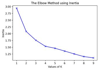
We collected all the hotwater consumption data of the location since it was put into use from September 2019 until June 2021. There are in total 547 daysof effective data. It can be seen fromthe figure that the curvestarts decreasing linearlyfrom k= 4. Therefore, the optimalnumber of clusters is4.
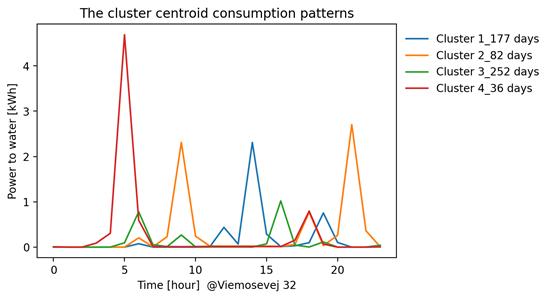
Then the K-means clustering with DTW distancewas carried out for all the data. The four cluster centroids are shown in Figure A-2.It can be seen that the four clustersare identified according to their peak patterns and the energy consumption intensity.
39
Figure A-1 The Elbow method using inertia.
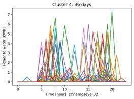
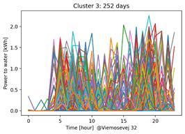
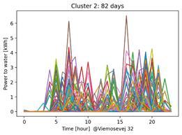
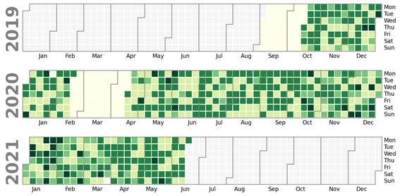
The daily curvesin each cluster are plotted in below figure.A cluster distribution map isshown in Figure A-4.6-1. It shows how the house’s daily hot water consumption profile changescluster throughout the period.The Nan days indicatesthe daysthatthe hotwater consumption wasnot correctlyrecorded and theywere removed from theclustering calculations.
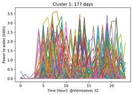
40
Figure A-2 The cluster centroid consumption patterns.
Figure A-3 Cluster 1-4.
41
Figure A-4.6-1 Cluster distribution map based on the measurements from House 1.
FUTURessourcer nergiE