MARCH

MARCH
HISSN 2837-5696
HYDROVISIONS is the official publication of the Groundwater Resources Association of California (GRA). GRA’s mailing address is 808 R Street. Suite 209, Sacramento, CA 95811. Any questions or comments concerning this publication should be directed to the newsletter editor at hydrovisions@grac.org
The Groundwater Resources Association of California is dedicated to resource management that protects and improves groundwater supply and quality through education and technical leadership.
EDITOR
Rodney Fricke hydrovisions@grac.org
EDITORIAL LAYOUT
Smith Moore & Associates
EXECUTIVE OFFICERS
PRESIDENT
Christy Kennedy
Woodard & Curran
Tel: 925-627-4122
VICE PRESIDENT
Erik Cadaret
Yolo County Flood Control & Water Conservation District
Tel: 530-756-5905
SECRETARY
Abhishek Singh
INTERA
Tel: 217-721-0301
TREASURER
Rodney Fricke
GEI Consultants
Tel: 916-407-8539
DIVERSITY, EQUITY AND INCLUSION OFFICER
Annalisa Kihara
State Water Resources Control Board
IMMEDIATE PAST PRESIDENT
R.T. Van Valer
ADMINISTRATIVE DIRECTOR
Amanda Rae Smith
Groundwater Resources Association of California asmith@grac.org
To contact any GRA Officer or Director by email, go to www.grac.org/board-of-directors
DIRECTORS
Jena Acos
Brownstein Hyatt Farber Schreck
Tel: 805-882-1427
Christopher Baker
DWR
Tel: 562-331-4507
Matthew Becker
California State Univ. Long Beach Tel: 562-985-8983
Trelawney Bullis
AC Foods, Central Valley
Tel: 530-205-8387
Dave Ceppos
Public Policy Mediation and Facilitaion
Tel: 916-539-0350
Elie Haddad
Haley & Aldrich Tel: 408-529-9048
Dr. Hiroko Hort
GSI Environmental, Inc
Marina Deligiannis Stantec
Tel: 916-418-8242
Clayton Sorensen
West Yost Associates
Tel: 925.949.5817
Melissa Turner
MLJ Environmental Tel: 530-756-5200
Savannah Tjaden
Environmental Science Associates
Tel: 208-350-3566
Roohi Toosi
APEX Environmental & Water Resources
Tel: 949-491-3049
John Xiong
Haley & Aldrich, Inc.
Tel: 714-371-1800
The statements and opinions expressed in GRA’s HydroVisions and other publications are those of the authors and/or contributors, and are not necessarily those of the GRA, its Board of Directors, or its members. Further, GRA makes no claims, promises, or guarantees about the absolute accuracy, completeness, or adequacy of the contents of this publication and expressly disclaims liability for errors and omissions in the contents. No warranty of any kind, implied or expressed, or statutory, is given with respect to the contents of this publication or its references to other resources. Reference in this publication to any specific commercial products, processes, or services, or the use of any trade, firm, or corporation name is for the information and convenience of the public, and does not constitute endorsement, recommendation, or favoring by the GRA, its Board of Directors, or its members.
President’s Message Page 4
Certified Hydrogeologists Page 6
CA Groundwater Supply
PFAS in Background
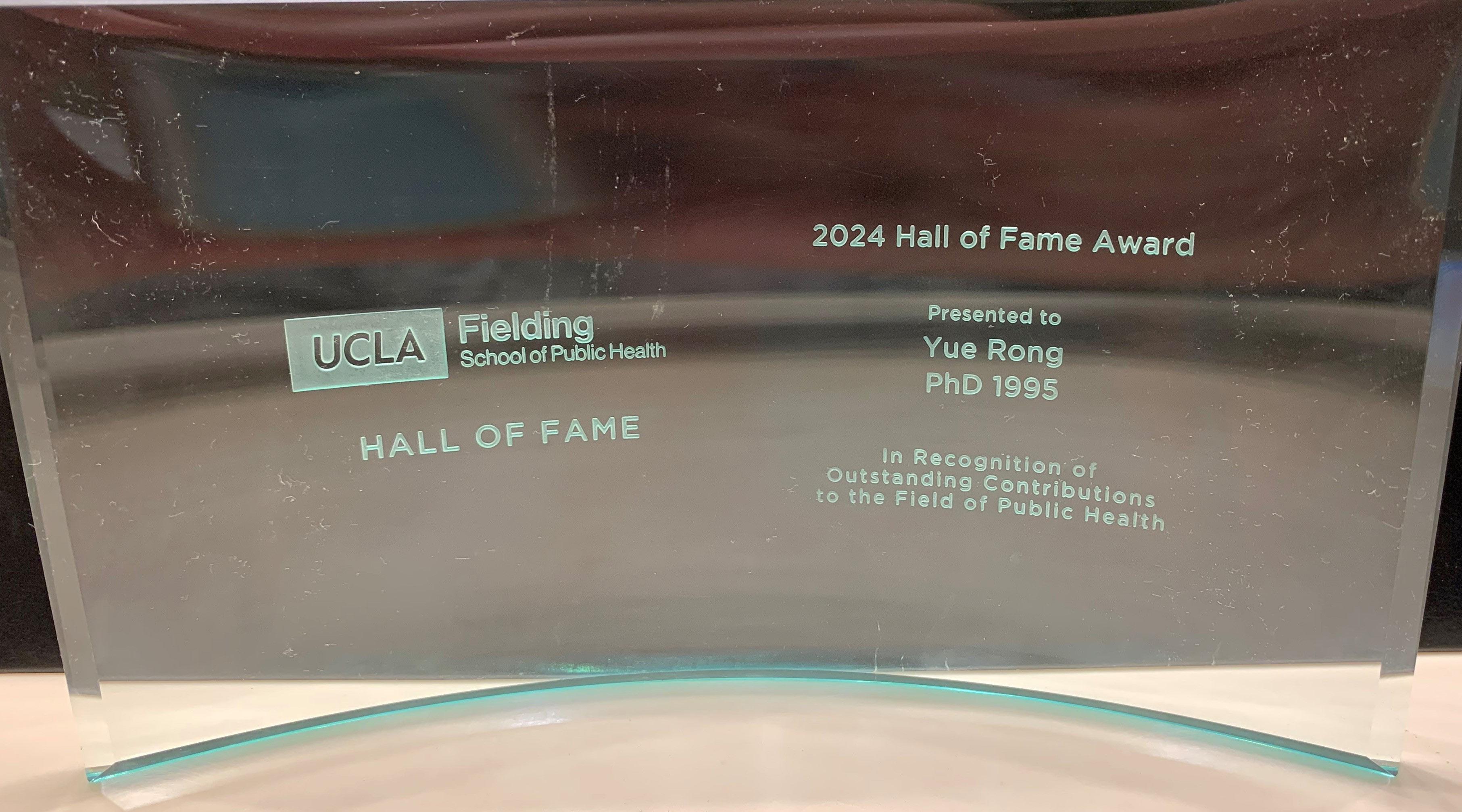
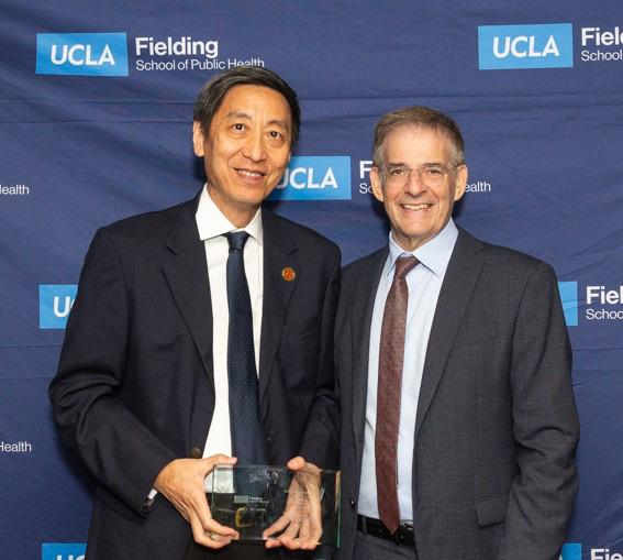
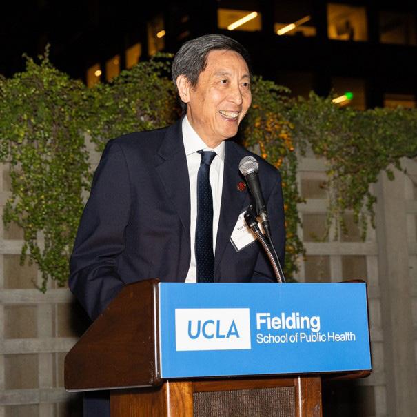
Yue Rong Induction
GeoH2OMysteryPix
Upcoming Events!
ISSN 2837-5696 c ontents
6 Certified Hydrogeologists How many? Where?
8 Early groundwater supply in California: From flowing artesian wells to heavy-lifting wells
12 PFAS Article #12: PFAS in Background
Dear GRA Members,
As we say goodbye to the winter season, and welcome the spring season, I want to address the significant federal water policy developments that unfolded last month and their implications for our groundwater community. The Executive Order “Emergency Measures to Provide Water Resources in California and Improve Disaster Response in Certain Areas” issued by The Republican Administration in January, presents both challenges and opportunities that deserve our attention.
Our Changing Water Landscape

The central reality we face is that while groundwater regulation remains primarily under state control, the administration’s directives to increase water deliveries to Central Valley Project (CVP) contractors will inevitably affect groundwater conditions throughout California. This interconnection between federal surface water management and local groundwater resources will shape our work in the months and years ahead.
For those of us dedicated to groundwater science, management, and protection, these developments have several important implications:
The Surface-Groundwater Relationship Is More Critical Than Ever
With the administration’s focus on delivering more water to CVP’s 250+ contractors across 29 counties, we can expect shifting patterns in surface water availability. This change in availability will directly impact groundwater recharge patterns, extraction rates, and basin dynamics. Your expertise in understanding and modeling these complex interactions will be increasingly valuable to water managers throughout the state.
SGMA Implementation Faces New Variables
Many Groundwater Sustainability Agencies (GSA) have developed plans based on certain assumptions about surface water availability. As federal policies potentially alter these patterns, GSAs will need support in adjusting their groundwater sustainability plans. These adjustments create opportunities for our members to provide technical guidance through this adaptation process.
Monitoring and Assessment Needs Will Expand
As agencies seek to understand how changes in federal water operations affect local groundwater conditions, demand for sophisticated monitoring, data analysis, and assessment will grow. Those of you working in groundwater monitoring technologies and data management will likely see increased interest in these services.
Collaboration Is Essential
Now more than ever, effective groundwater management will require cross-disciplinary collaboration. GRA is already expanding our efforts to facilitate dialogue between groundwater professionals, surface water managers, policy experts, and stakeholders to navigate these challenges collectively.
Looking Forward
While these developments present challenges, they also highlight the essential role our members play in California’s water future. Your scientific expertise, technical knowledge, and commitment to sustainable groundwater management have never been more important. The Groundwater Resources Association remains committed to supporting you through educational programs, policy updates, and networking opportunities as we adapt to this evolving landscape. Our upcoming SGMA Summit and Law & Legislation Forum in May will feature topics around navigating the implications of federal water policy changes for groundwater management, and I hope to see many of you there.
We know we are later than normal getting our winter edition out, but holidays always make things busy. We look forward to getting our publication back on track this year and providing you more new and informative content on the groundwater world.
As always, I welcome your thoughts, questions, and insights on these issues. Together, we will continue our work toward sustainable groundwater management, regardless of the changing political landscape.
Sincerely,
Christy Kennedy


by Rodney Fricke, CHG 11
Hydrogeologists appear to be in demand these days, if I can trust social media and the weekly emails that I was receiving during late 2024 looking for hydrogeologists. A California certification adds to your qualifications to pursue such opportunities. I took the first exam in 1995 and was fortunate to become Certified Hydrogeologist #11 because I showed up at the office of the BPELSG1 shortly after 8:00 on 10-Jul95 and got in line with five other successful applicants (#8 through #12). The first seven certifications were established by an internal BPELSG process, based on their prior experience as Professional Geologists (PG) / Certified Engineering Geologists (CEG), so they could create that first test.
I recently checked the lookup function on the BPELSG website and found a link to download the entire database of licenses – 119,341 entries through the end of 2024, including 11,860 delinquent licenses which means the license has expired and renewal is past due. Hydrogeologists account for 96 delinquencies.
Focusing on the active licenses, my count totaled 105,278 licenses, mostly Engineers (92%), primarily civil (55%), mechanical (15%), or electrical (11%) plus 16 other engineering licenses (12%), along with Professional Geologists (4.7%), Land Surveyors (3.7%), and stand-alone2 Professional Geophysicists (0.1%). My count did not include CEG or Certified Hydrogeologist (CHG) because those certifications require a PG license. Of the 4,958 active PGs, 1,309 are CEGs (26%) and 858 are CHGs (17%). I’d like to mentions that nine professionals have all four “geo” licenses and I’m thinking that some PGs might also be engineers.
The highest CHG license number was found to be 1126 so accounting for the active (858) and delinquent (96) licenses means that 172 CHG licenses have been cancelled since 1995.
Of the 858 active CHGs, 708 are located in California and 150 are located out-of-state, including two in Canada and one in France. Approximately 15% of the active CHGs are female.
Figure 1 shows the CHG count per county using several colors to distinguish the eight GRA branches. CHGs are based in 42 of the 58 counties, mostly in southern California – Orange County hosts the most CHGs (107), followed by
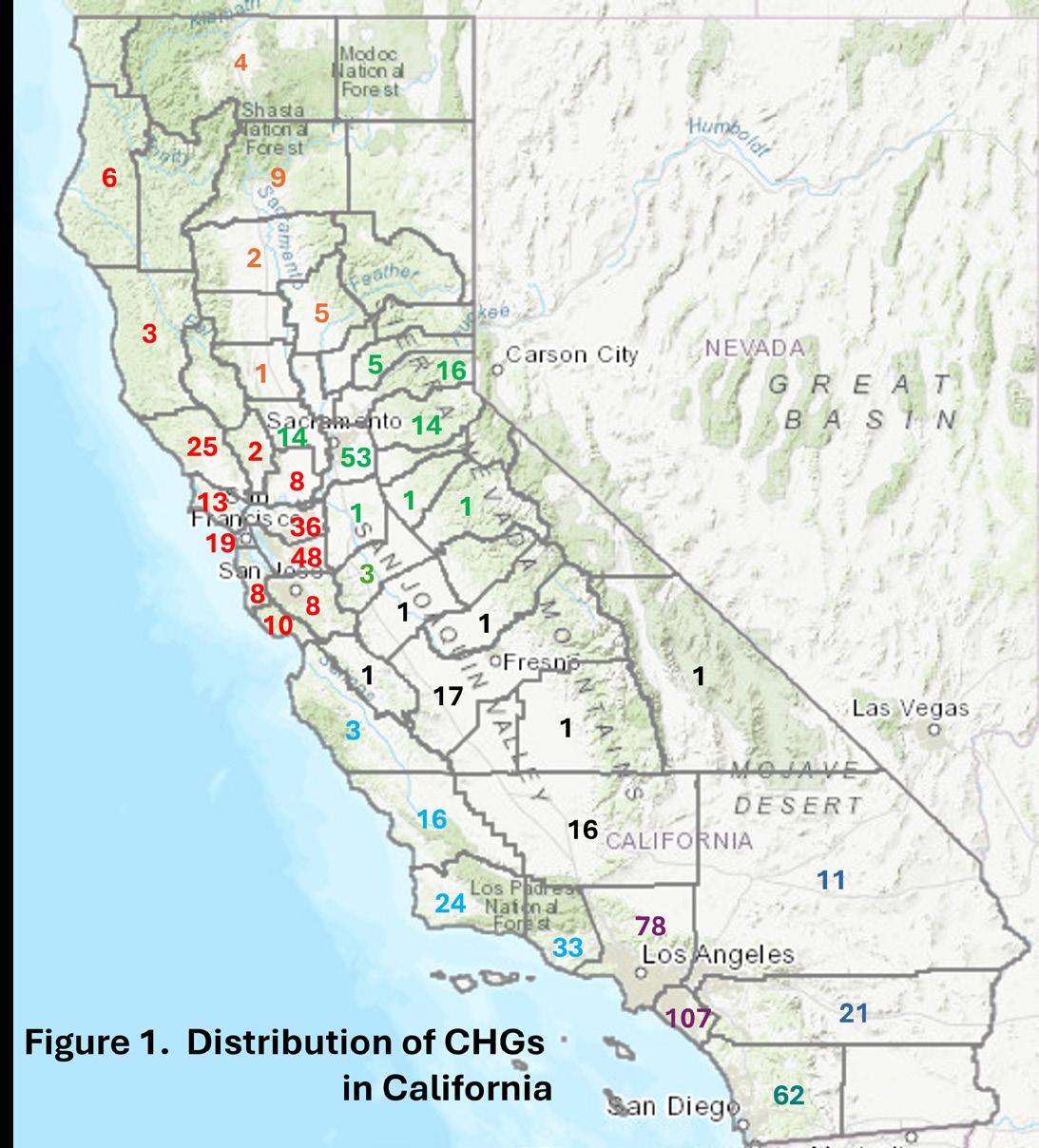
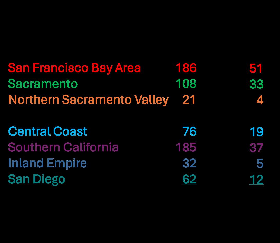
Los Angeles (78) and San Diego (62) counties. In northern California, Sacramento County leads the CHG count (53), followed by Alameda (48) and Contra Costa (36) counties. Table 1 summarizes the CHG count for each of the eight GRA branches plus out-of-state CHGs. The highest CHG counts were found in the San Fransico Bay Area branch (186) and in the Southern California branch (185) as would be expected from their large metropolitan populations.
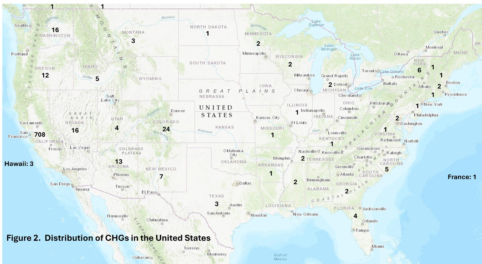
Figure 2 shows the count for CHGs that reside in 32 other states across the country. As might be expected, most of these CHGs (60%) are found in western states, including Colorado (24), Nevada (16), Washington (16), Arizona (13), Oregon (12), and New Mexico (7).
I cross referenced the CHG database with the GRA database and found that only 192 active CHGs were listed as GRA members – less than 25%. As shown by Table 1, the San Francisco Branch has the most CHG-GRA members (51), followed by the Southern California Branch (37), the Sacramento Branch (33), and the Central Coast Branch (19). Out-of-State CHG account for 26 GRA members, including Colorado (7), Washington (4), and New York (4) and seven other states.
1 Board of Professional Engineers, Land Surveyors, Geologists, and Geophysicists
2 Numerous Professional Geophysicists are also Professional Geologist, Certified Engineering Geologist and/or Certified Hydrogeologist and were counted as Professional Geologists. A total of 146 Professional Geophysicists are licensed in California.
by Hugo A. Loaiciga, Ph.D. P.E. B.C. WRE, P.H., Director Hydrology Laboratory, University of California, Santa Barbara
This essay provides a brief historical account of groundwater provision for agricultural and urban uses in the period 1878 through 1890 (the early years, henceforth). Data were collected from several sources, but mainly from the 1894 report by Special Agent Frederick H. Newell (Newell, 1894). Newell would become Chief Hydrographer of the USGS Hydrography Division and later Chief of the Reclamation Service. He was hired in 1888, when Major John Wesley Powell was serving as the second director of the USGS. Powell led expeditions through the Colorado River between 1869 and 1874 and published in 1879 (the year in which the USGS was created) the influential “Report on the Arid Lands of the United States”. The Powell report provided intellectual impetus for the enactment of the 1902 federal Reclamation Act that funded water storage and irrigation projects in the arid lands of the western United States in general, and in California in particular (e.g., the Central Valley Project). The story narrated in this essay corresponds to a time when California’s population was 1,208,130 (according to the 1890 census), compared to the approximately 39.2 million inhabitants in 2024. There were 1,004,233 acres of irrigated land in California according to the 1890 census, compared with the current 7.8 million acres in 2024 (USDA National Agricultural Statistics Service). Most of the irrigation and urban water in the early years came from stream diversions, although some was provided by wells. The average “first cost” (i.e., the cost of diversion and conveyance) of water derived from gravity supplies for the whole United States was $8.15 per acre foot, varying between $3.62, the average for Wyoming, and $12.95, the average for California (Newell, 1894).
Three counties (San Bernardino, Kern, and Sacramento) were herein chosen to describe groundwater supply in the early years in California. The chosen counties represent the diverse geography of the State and have supported agriculture for many generations. It is stressed in the following that most wells in the early years were flowing artesian wells, where the water level within the well rises naturally above ground level thus bypassing the need for water lifting by artificial means. A common method for lifting water in non-flowing wells in the early years in California, and elsewhere in the United States, was the windmill outfitted with a suction pump. The windmill with suction lift could raise groundwater between 25 and 30 feet according to basic hydraulic considerations (Hood, 1898; Barbour 1899). The cost of windmills averaged between $ 50 and $ 400 nationwide according to size and make (Wilson, 1896). There were in the early years several rudimentary machines to lift water: lift pumps, force or plunger pumps, rotary and centrifugal pumps, and mechanical or siphon elevators. The motive power to drive these machines was derived from various sources: animal, wind, water, hot air, explosive force of gas, and steam. Notoriously absent in the early years was electric power, which in the early 1900s revolutionized groundwater pumping with the introduction of the deep-well vertical turbine pump and multistage centrifugal pumps. The reader is referred to the USGS Water Supply Paper and Irrigation Paper No. 1 (Wilson, 1896) and to the USGS Water Supply and Irrigation Paper No. 29 (Barbour, 1899) for insightful descriptions of water supply in the United States before the advent of electricity and electric-powered pumps.
Groundwater supply in San Bernardino County (abridged and modified from Newell, 1894). This county extends from the Colorado River and the state line of Nevada on the east westward to Kern County, Los Angeles County and Orange County. By far the greater part of the county is located within the Colorado or Mohave Desert, the southwestern prolongation extending over the lofty mountains down into the valleys drained by the Santa Ana River and other streams flowing to the sea. It is in this relatively small portion of the county that were concentrated nearly all the population and wealth of this, the largest, political division of the State. San Bernardino County had some of the best examples of irrigation development to be found in the United States. These water systems were notable for the elaboration of details and the care and expense lavished in saving and utilizing the water resources. There were water-storage reservoirs, carefully built ditches, many of them paved and cemented, tunnels, flumes, pipes of cement, iron, and steel, many devices for measuring, dividing, and distributing the water. In short, examples of nearly every type of irrigation works, from the crudest to the latest improvements. In the point of cost and thoroughness of construction, these irrigation works were comparable with those built for municipal supply, bringing water under pressure to the houses and to the orchards. A total of 301 artesian farm wells were enumerated in San Bernardino
county in 1890, ranging from 65 to 700 feet in depth, and having an average discharge of 283 gpm. The water of many of the larger of these wells was piped to various towns, giving them an ample supply of clear, pure water. A few of the wells were used for purposes of irrigation, an average of 20 acres being watered by each well thus employed. A large number of wells were drilled by land companies to ascertain the extent and amount of the artesian supply, and the resources of the county in this direction were well explored. A few farmers complained that these large wells, which were allowed to flow freely for months or years, resulted in the drying up of the shallow wells near the edge of the basin. In neighboring Los Angeles County, certain wells were installed as early as 1870, and their rapid increase in number had the effect of diminishing pressure and flow from some of the older wells. These are the earliest reports of well interference in California (Newell, 1894). This evidence of well interference shows that the conditions needed to maintain flowing artesian groundwater are highly sensitive to the volume of groundwater extraction from an aquifer tapped by wells. Table 1 provides details of the five most productive wells within an artesian area in the vicinity of the Santa Ana River in San Bernardino County. These were called the Gage Canal wells for their proximity to the canal so named. The measurements of capacity listed in Table 1 were made at the
on next page
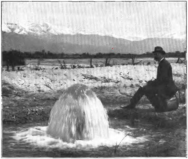
end of the irrigating season while all the wells were open and after they had been flowing freely during the summer. The pressure, expressed as that exerted by a column of water (in feet), was measured in each well while it was closed. Figure 1 displays a photograph of well number 43, the most productive among the Gage Canal wells.
Groundwater supply in Kern County (abridged and modified from Newell, 1894). This county is in the extreme southern end of San Joaquin Valley, extending from the coast range easterly across the end of the valley to and beyond the Sierra Nevada mountains, and including in its southeastern corner a portion of the Mohave desert, a part of the great interior basin of western United States. The most valuable agricultural lands of the county were within the San Joaquin basin between the lowest ground and the foothills of the Sierra Nevada. The Kern River and other streams flowing westward from the Sierra Nevada provided most of the irrigation water in Kern County in the early years. Those surface-water supplies have ever since been augmented by the State Water Project and the federal Central Valley Project.
Kern County had numerous flowing artesian wells and a large quantity of water was discharged by them in the early years. The principal flowing artesian wells that existed are shown as small, empty circles, in Figure 2. They were located mainly within townships 25, 26, and 27 south, and ranges 22, 23, and 24 east, relative to the Mount Diablo meridian. There were also many flowing artesian wells in the lower part of what is known as the Kern delta, south and southwest of Bakersfield. The largest flowing artesian wells were in township 27 south, range 23 east this being about 40 miles southeasterly from Tulare Lake. In this township, the Kern County Land Company had 24 flowing artesian wells, varying in depth to bottom from 300 to 1,100 feet, and 4 wells not flowing (i.e., standing artesian wells), with depths to bottom varying from 400 to 1,000 feet. The discharge in most flowing artesian wells ranged from 40 to 420 gallons per minute (gpm), but a few wells discharged as much as 1,700 gpm. The cost of these wells varied from $2 to $3 per foot in depth. One of the largest wells was in section 17, township 26 south, range 23 east and was 635 feet deep, 8 inches in diameter, and cost $1,875. It
discharged at the rate of 1,660 gpm and irrigated 320 acres of young orchards of plum and fig trees, raisin vines, grains, alfalfa, corn, sorghum, vegetables, and shade trees. Taking Kern County as a whole, the average depth of the wells was 551 feet, diameter 8 inches, and cost $1,489. The discharge was 1,072 gpm, and the average area irrigated by each well was 125 acres.
Groundwater supply in Sacramento County (abridged and modified from Newell, 1894). This county includes a portion of the central part of Sacramento Valley, east of the Sacramento River and extending to the foothill regions. The greater part of the area is less than 100 feet above sea level and, on the western and southwestern sides, the lands in their original condition were overflowed and marshy. Extensive systems of dikes were built, reclaiming valuable tracts whose surface was covered by a soil of wonderful fertility. Adjoining this area are lands at a slightly greater altitude that were kept moist by the presence of the groundwaters saturating the subsoil or lower layers. Still further to the east are the higher grounds, also of great fertility, but subject to summer droughts. Irrigation was practiced to a relatively small extent, since all the cereals were successfully raised upon the broad plains. Water was employed mainly for orchards and vineyards on the higher grounds of the county. Water for a large proportion of the irrigated orchards was obtained from wells where the depth to water varied from 10 to 40 feet. Groundwater was pumped by means of windmills or by steam or horse power. The wind was commonly depended upon from April to August, but in the latter part of the summer was often light and fickle. In other respects, this method of obtaining water was usually preferred by owners of small orchards. The cost of the windmills ranged from $75 to $110, of pumps from $15 to $40, and it was about $1 per foot in depth or less for shallow wells. In this county, there were several deep wells, but it is doubtful whether any of them was artesian. On Tyler Island, 30 miles south of the City of Sacramento, was a well 102 feet deep, in which water rose to within 6 feet of the surface. Near Arcade, about 8 miles northeasterly from Sacramento, a well was drilled to the depth of 2,160 feet, at a cost of $30,000, but without success so far as flowing water is concerned. Other wells near Sacramento were drilled nearly 600 feet deep with the same result. West of Sacramento, near Davis and Woodland, in Yolo county, wells were drilled to depths of 200 feet or deeper. The water in these wells rose nearly to the surface, and one well flowed during part of the year.
To conclude, it is difficult to believe that groundwater supply in California’s early years was primarily made by flowing artesian wells, a situation nowhere to be seen nowadays. In the early years, California was largely an agrarian society relying on rudimentary technology. Well-installation and watersupply costs were low compared to today’s values, even after accounting for the time-change of money. Well interference emerged in the early years in the Golden State as wells proliferated near each other, a harbinger of things to follow in the coming decades.
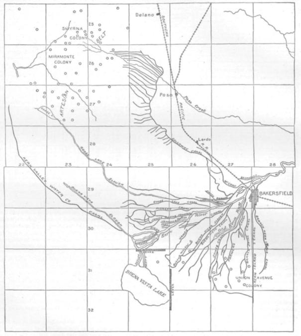
Figure 2. Map displaying artesian wells (shown as empty circles) in Kern County in the early years. Notice the Kern River and numerous diversion canals near the City of Bakersfield. (Source: Newell, 1894). Kern lake was reclaimed (dried up) and Buena Vista Lake’s size represents a reduction of its natural size before reclamation.
References
Barbour, E.H.1899. Wells and windmills. USGS Water Supply and Irrigation Paper No. 29. Government Printing Office, Washington, D.C.
Hood, O.P. 1898. Certain pumps and water lifts used in irrigation. USGS Water Supply and Irrigation Paper No. 14. Government Printing Office, Washington, D.C.
Lippincott, J.B.1902. Development and application of water. San Bernardino, Colton, and Riverside, California. Water Supply and Irrigation Paper No. 92. Government Printing Office, Washington, D.C.
Newell, F.H. 1894. Report on agriculture by irrigation in the western part of the United States at the Eleventh Census, 1890. Government Printing Office, Washington, D.C.
Wilson, H.M. 1896. Pumping water for irrigation. USGS Water Supply and Irrigation Paper No. 1. Government Printing Office, Washington, D.C.
by John Stults, Dan Bryant, Azita Assadi, Stefanie Shea and Meeta Pannu
PFAS are ubiquitous in the environment as a direct result of the numerous applications of PFAS since the middle of the 20th century to the present. The distinct chemical nature of each individual PFAS along with the diversity of PFAS types (i.e. short-chain, long-chain, telomers, etc.) enable these substances to partition into various environmental matrices, including soil, air, groundwater, surface water, and rainwater. Transport modeling and soil concentration data suggest that PFAS emitted to air may be transported hundreds of kilometers from sources. Since PFAS presence is widespread and poses health risks even at very low levels, commercial labs have rapidly developed the ability to detect PFAS at nanograms per liter (ng/L) or parts per trillion (ppt) levels in aqueous matrices. An unintended consequence of the rapid development in PFAS analytical detection capabilities is that almost every environmental sample is found to contain low levels of PFAS, which can be referred to as “background” PFAS concentrations, no matter how distant the sample location is from a potential PFAS source.

Knowing background concentrations is important to inform our understanding of baseline levels of contamination that can be expected in areas that are not impacted by on-site discharges (i.e., non-impacted areas). To properly assess the risks of PFAS exposure and decide on cleanup actions at contaminated sites, it’s important to differentiate between levels of contamination associated with diffuse inputs from far-removed sources (anthropogenic background) and levels that are harmful enough to require cleanup (actionable contamination levels).
A historical meta-analysis of >21,000 concentration measurements of PFOS and PFOA found that groundwater concentrations ranged from 0.01 ng/L to 5 milligrams per liter (mg/L) – over 8 orders of magnitude (Johnson et al. 2022). By classifying groundwater into three source types (primary source, secondary source, and no known source), Johnson and co-workers were able to effectively determine probable ranges of background concentrations in groundwater for 27 target PFAS. At background sites, short-chain PFAA concentrations tended to be < 10 ng/L, while long chain PFAAs and telomer sulfonates tended to be <1 ng/L. Notable exceptions are PFOS and PFOA, which tended to have higher concentrations relative to all other PFAS regardless of primary source site.
Since 2006, the Minnesota Pollution Control Agency has monitored PFAS in 276 wells within the Ambient Groundwater Monitoring Network. In a study to assess the anthropogenic background level of PFAS, 50 wells screened between <25 and <75 feet below ground surface in areas with no known proximal sources of PFAS were monitored. Detection limits for all PFAS were approximately 2 ng/L and found that most wells had no detectable PFAS. Only PFBA (3 of 50), PFBS (1 of 50), and PFOA (1 of 50) were detected below 10 ng/L. The exception was PFBA, the most mobile of the PFAS analyzed, which had measurable concentrations above 10 ng/L.
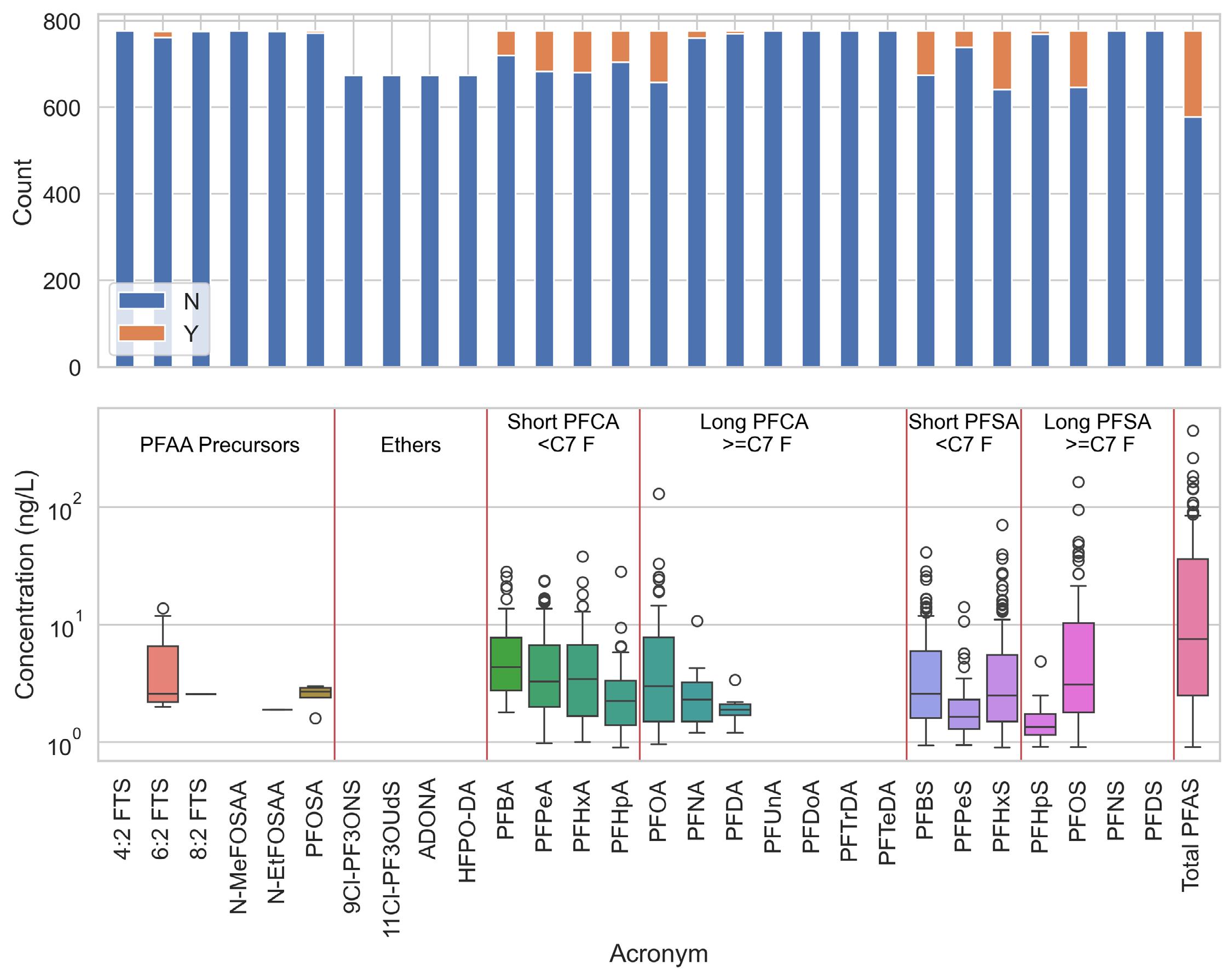
The USGS maintains a database of PFAS concentrations in groundwater samples collected by California Groundwater Ambient Monitoring and Assessment. Samples were collected between 2019 and 2023 from drinking and public water supply wells from priority basins and include secondarysource sites (Voss et al.,2023). Results from this dataset are analyzed and presented in Figure 1 below.
article continues on next page
Results from Voss et al. (2023) show the vast majority of PFAS detections in background sources are C3 perflurobutanoate (PFBA) through C8 perfluorononate (PFBA), which are perfluorocarboxylates (PFCAs); and C4 perfluorobutane sulfonate (PFBS) through C8 perfluorooctane sulfonate (PFOS), which are perfluorosulfonates (PFSAs). Of the 768 individual samples in this study, 198 (26%) had at least one detectable PFAS. Measurable PFAS concentrations were generally less than 10 ng/L.
PFAS are highly mobile in the atmosphere, as they can attach to particulate matter through gas-particle partitioning, allowing them to travel long distances via wind currents and be deposited far from their original sources through both wet and dry deposition (Faust, 2023).
PFAS deposition through precipitation can be a human exposure pathway, particularly in arid regions that rely on rainwater for various uses. Rainwater capture and managed aquifer recharge are common practices in areas like California, where water scarcity is a concern. By capturing and infiltrating rainwater into the soil, these systems help reduce stormwater runoff, mitigate flood risks, and enhance groundwater supplies. However, the atmospheric transport and subsequent deposition of PFAS through rainwater can lead to PFAS impacts even in areas that are not directly near a source.
In rainwater samples collected across the United States, the shorter-chain PFAS appears to be in higher concentration than the longer-chain PFSAs; the PFCAs are measured more frequently than PFSAs. The total PFAS concentration in rainwater reported in five studies published since 2021 ranged from 2.28-92 ng/L (Coates and Harrington, 2024). The study samples were collected from rain waters in Wisconsin, Ohio, Indiana, Wyoming, Arizona and Massachusetts. PFAS concentrations in rainwater are not available for California. Geographic regions and population densities are generally poor predictors of PFAS concentrations in rainwater (Olney et al., 2023), but local point sources can be important predictors for the concentrations and chemistries measured in rainwater (Pike et al., 2021).
PFAS concentrations in rainwater are influenced by cloud and precipitation processes. PFAS were more frequently detected in rainfall from convective rain events - which are typically characterized by intense localized thunderstorms - compared to stratiform rain events, which are generally broader and more gradual weather systems (Olney et al., 2023). Additionally, PFAS concentrations tend to be higher in the initial stages of rainfall events, which suggests the PFAS scavenging rates decrease with storm duration (Kwok et al., 2010). Consideration of the type and magnitude of precipitation events is important when assessing the spatial and seasonal variability of PFAS from rain and resulting background concentrations.
PFAS are detected in surface soil worldwide, including remote locations far from industrial sources (Brusseau et al., 2020). The background soil levels show certain patterns worldwide. For example, as a group, PFCAs (such as PFOA) are predominant over PFSAs (such as PFOS) (Brusseau et al, 2020; Ma et al., 2022). The predominance of PFCAs in soil most likely reflects the large suite of precursors known to degrade to PFCAs during atmospheric transport and the corresponding more common detection of PFCAs in precipitation (Kwok et al., 2010; Pike et al., 2021).
The most frequently detected PFAS, and the PFAS typically detected at the highest concentrations, in surface soil were PFOS and PFOA. Worldwide median maximum concentrations at sites with no known sources were 2.7 micrograms per kilogram (ug/kg) for both PFOS and PFOA, and maximum concentrations were 162 ug/kg for PFOS and 124 ug/kg for PFOA (Brusseau et al., 2020). For sites in the United States, the median maximum concentrations were 9.7 ug/kg for PFOS and 4.9 ug/kg PFOA, and maximum concentrations were 126 ug/kg for PFOS and 33 ug/kg for PFOA. The predominance of PFOS and PFOA relative to other PFAS in North America is at first puzzling because manufacture of both compounds and precursors that can transform to them ended in approximately 2002 and 2015, respectively. PFOS and PFOA were replaced by shorterchained PFAS in North America, thus relatively higher concentrations of those shorter-chained PFAS may be expected in surface soil. Manufacture of both PFOS and PFOA, however, has continued outside North America. Global atmospheric circulation modeling suggests that those sources outside North America are atmospherically transported to North America (Thackray et al, 2020), which may account for the continued predominance of PFOS and PFOA.
The anthropogenic PFAS soil background can also pose regulatory issues. Systematic studies of surface soil background PFAS concentrations across northern New England (McIntosh et al., in review) have shown that the anthropogenic background concentrations are often in the range of 2-3 ug/kg. While lower than direct exposure concentrations, these concentrations may exceed soil cleanup standards intended to limit PFAS leaching to groundwater. Thus, property owners could be responsible for investigation and remediation even though no onsite release has occurred. Given the ubiquity of PFAS today, soil anthropogenic background concentrations should be considered during promulgation of cleanup standards.
PFAS contamination is a widespread environmental and health concern, with these substances found in various media including rainwater, soil, and groundwater. Detection of low levels of PFAS in areas that are not impacted by on-site discharges (non-impacted areas) is an unintended consequence of the rapid development in PFAS analytical detection capabilities. Differentiating between anthropogenic background levels and contaminated sites requiring remediation is essential for effective risk assessment and regulatory action.
Continued research and monitoring are crucial for understanding PFAS distribution and mitigating their impact on public health and the environment.
References:
1. Brusseau, M. L., et al. (2020). PFAS depth profiles and soil contamination. Journal of Contaminant Hydrology, 228, 103556.
2. Coates, J., & Harrington, J. (2024). PFAS concentration in rainwater across the United States. Environmental Science & Technology, 58(3), 1456-1463.
3. Faust, S. (2023). Atmospheric transport and deposition of PFAS. Environmental Pollution, 264, 114763.
4. Johnson, G. R., Brusseau, M. L., Carroll, K. C., Tick, G. R., & Duncan, C. M. (2022). Global distributions, source-type dependencies, and concentration ranges of per- and polyfluoroalkyl substances in groundwater. Science of The Total Environment, 841, 156602.
5. Kwok, K. Y., et al. (2010). Detection of PFAS in rainfall from different weather events. Atmospheric Environment, 45(6), 11901198.
6. Ma, J., et al. (2022). Global patterns of PFAS in soil. Science of the Total Environment, 832, 155041.
7. McIntosh, L., Rockwell, C., Olney, S., Campe, L., Collins, R.D., Bryant, J.D., Ward, T., Harring, P., & Occhialini, J. (2025). Background PFAS concentrations in surface soil of Massachusetts and northern New England: Regional and global source patterns and regulatory relevance. Remediation Journal, 35: e70013. https://doi.org/10.1002/rem.70013
8. Minnesota Pollution Control Agency. (2024). Monitoring PFAS in ambient groundwater. Minnesota Pollution Control Agency Annual Report.
9. Olney, T. R., et al. (2023). Predictors of PFAS concentrations in rainwater. Water Research, 243, 116873.
10. Pike, E. R., et al. (2021). Influence of local point sources on PFAS in rainwater. Science of the Total Environment, 750, 141672.
11. Thackray, C. P., et al. (2020). Global transport and sources of PFAS in North America. Environmental Science & Technology, 54(8), 4783-4792.
12. Voss, S. A., Jurgens, B. C., & Kent, R. H. (2023). Data for Per- and Polyfluoroalkyl Substances (PFAS) in groundwater samples collected by the California Groundwater Ambient Monitoring and Assessment Priority Basin Project (2019-2023), U.S. Geological Survey Data Release. Retrieved from https://www.sciencebase.gov/ catalog/item/641b44f8d34e4c337f0c31d7

With offices in Sacramento, Oakland, Monterey, San Luis Obispo, and Pasadena, we specialize in:


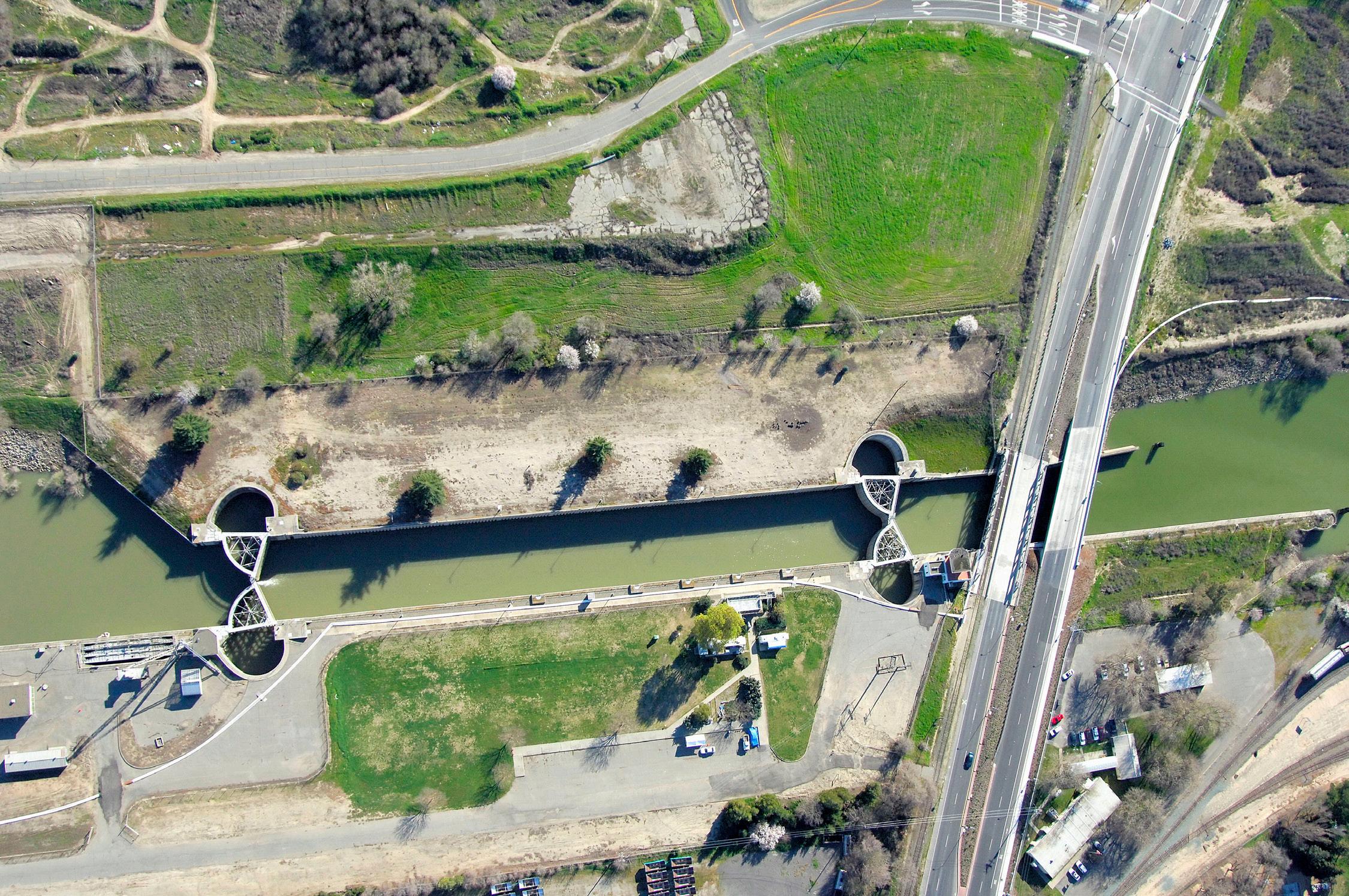
What is this? Where is it Located?
Hint: A unique West Coast facility.
Congratulations to Don Ashton, Sr. Project Manager, Apex Companies, LLC for providing the following correct response to the Summer 2024 GeoH2OMysteryPix questions:
“Your GeoH2OMysteryPix is of the Barge Lock at the Sacramento Harbor where the shipping channel connects to the main Sacramento River.”
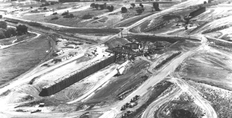
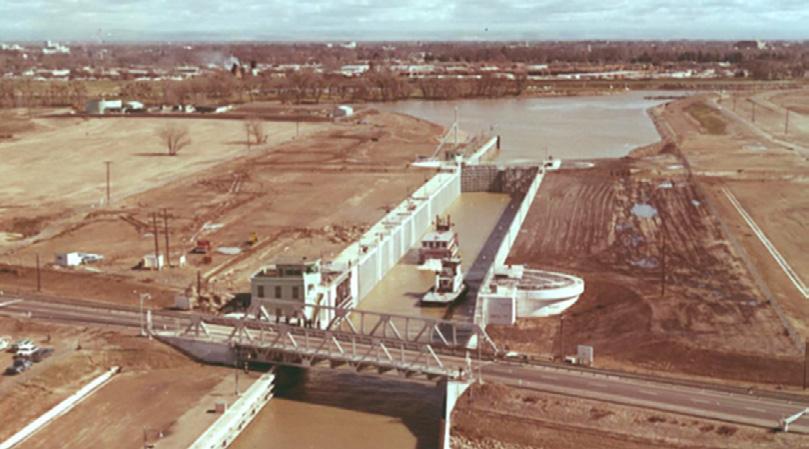
Background/History: The Stone Lock Facility, historically known as the William G. Stone Locks Facility, is a navigational lock facility built by the U.S. Army Corps of Engineers (USACE) in 1961 as part of the Deep-Water Ship Channel Project, authorized by the River and Harbor Act of
1946. The Facility was named after William G. Stone who was instrumental in persuading the USACE to study the navigation project, which eventually was constructed. The Sacramento Deep Water Ship Channel Project connects the Pacific Ocean to the Sacramento River, consisting of a deep-water ship channel, the Port of West Sacramento, a barge canal, a bascule bridge, and two sector gates forming a lock chamber (the Stone Lock Facility). The Deep Water Ship Channel Project consists of a 40-mile-long deep-water ship channel beginning at the head of the Suisun Bay near Collinsville, California, continuing north to the Port of West Sacramento, and then eastwardly through a barge canal and lock chamber, connecting to the Sacramento River.
The Stone Lock Facility is the most northeastern portion of the Deep Water Ship Channel Project and contains the navigational lock. Although the two sector gates are no longer operated for navigational purposes, the lock chamber was historically used for raising and lowering water levels so barges and other watercraft could pass between the Sacramento River and the Barge Canal. Although the Stone Lock Facility was federally decommissioned in 2000, it includes a removable flood wall feature, that when in place, provides flood protection from the Sacramento River during high-water events. In 2020, the City of West Sacramento completed a historical significance evaluation of the Stone Lock Facility that confirmed its eligibility for registration as a historical resource and property.
The Stone Lock Facility presents an opportunity to be preserved as a physical representation of its historically significant past, while becoming a regional attraction as part of the Stone Lock Plaza, an envisioned sub-area of the City’s future Central Park.
References:
ArcGIS 2022. Stone Lock Plaza Story Map. September 29: https://storymaps.arcgis.com/stories/756f490224724950b9372f91c90f6b37
2022. City of West Sacramento and West Sacramento Historical Society Archives.
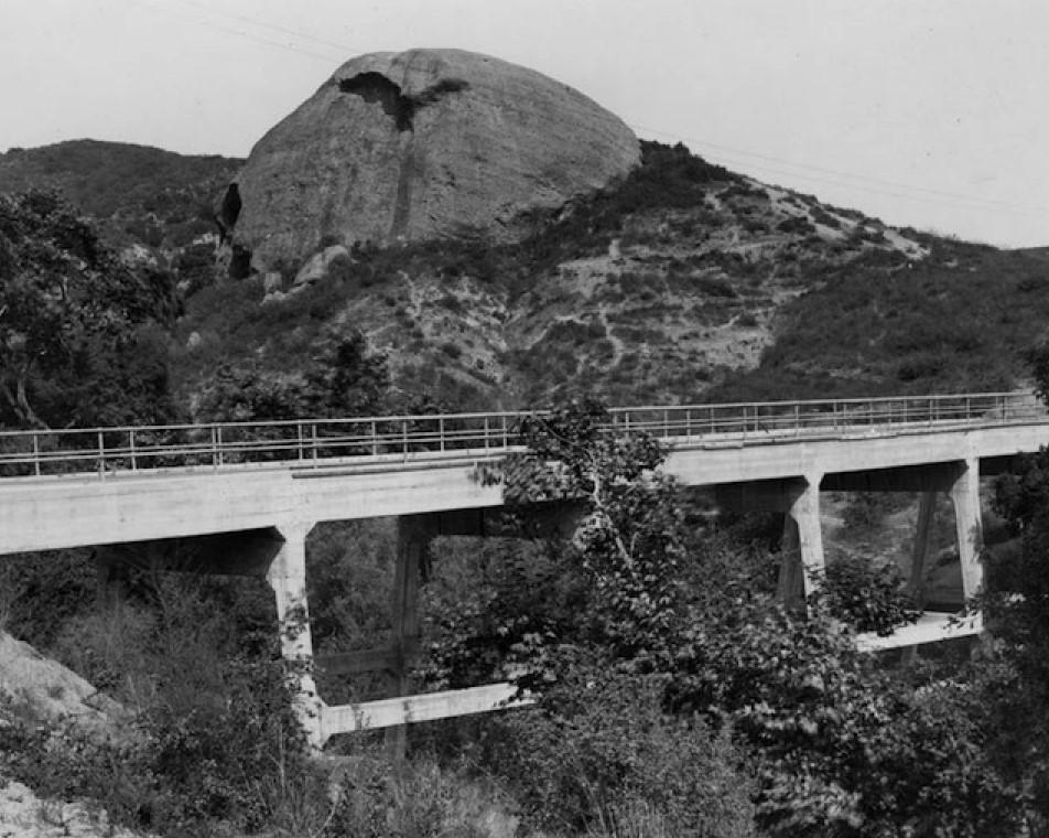
What is this? Where is it Located? Hint: A historic California landmark. Think you know What this is and Where it is Located? Email your guesses to Chris Bonds at goldbondwater@gmail.com
GRA has an exciting lineup of events designed to keep you informed and engaged with the latest developments in groundwater management. From policy discussions to technical innovations, our upcoming programs offer valuable insights and networking opportunities for water professionals across California and beyond.
Kicking off this spring, the SGMA Implementation and Legislative Summit will take place on May 27-28, 2024, in Sacramento. This essential event brings together policymakers, regulators, and industry experts to discuss the latest updates on the Sustainable Groundwater Management Act (SGMA). Attendees will gain critical insights into implementation progress, legislative priorities, and emerging challenges affecting groundwater sustainability across the state.
Looking ahead, GRA’s premier technical conference, the 2025 Western Groundwater Congress (WGC), is set for October 6-8, 2025, in Burbank, CA. The WGC is the go-to event for groundwater professionals, offering cutting-edge technical sessions, engaging panel discussions, and extensive networking opportunities. With topics ranging from groundwater quality and contamination to managed aquifer recharge and emerging technologies, this event is not to be missed.
Beyond these signature events, GRA continues to foster knowledge sharing and collaboration through monthly Branch Meetings. These regional gatherings provide a platform for groundwater professionals to discuss local challenges, exchange ideas, and stay up to date with the latest research and regulatory changes impacting groundwater management.
Additionally, GRA offers a robust lineup of GRACasts, featuring expert-led webinars on key groundwater topics. Whether you’re looking to deepen your technical expertise or stay informed on policy updates, these virtual sessions provide accessible, high-quality education for professionals across all sectors.
We invite you to take advantage of these opportunities to connect, learn, and advance your knowledge in groundwater management. Stay engaged by visiting grac.org for event details, registration, and updates on additional programming throughout the year.


Azita Assadi. P.Geo. is a technical committee member at the GRAC. She is a Hydrogeologist with over 20 years of consulting experience in water resources and soil/groundwater management in the US, Canada, and internationally. She is currently working as a Geologist at A-Tech Consulting Inc. in the field of subsurface investigation and water resources management.
Chris Bonds is a Senior Engineering Geologist (Specialist) with the California Department of Water Resources (DWR) in Sacramento. Since 2001, he has been involved in a variety of statewide projects including groundwater exploration, management, monitoring, modeling, policy, research, and water transfers. Chris has over 31 years of professional work experience in the private and public sectors in California, Hawaii, and Alaska and is a Professional Geologist and Certified Hydrogeologist. He received two Geology degrees from California State Universities. Chris has been a member of GRAC since 2010, a Sacramento Branch Officer since 2017, and has presented at numerous GRAC events since 2004.
Dan Bryant, PhD, is Woodard & Curran’s National Practice Leader for Emerging Contaminants. Dan has 28 years of geochemistry and in-situ remediation experience that crosses the spectrum from fractured bedrock to unsaturated shallow soil, with contaminants including metals, chlorinated solvents, petroleum hydrocarbons, explosives, PAHs, and emerging contaminants including 1,4-dioxane and PFAS. Dan has three issued and one pending patent for in-situ remedies for metals, chlorinated solvents, and PFAS. Dan is a licensed geologist in Missouri, Georgia, New York, and Indiana. He has bachelor's and master's degrees in geology from the University of Florida, and master’s and Ph.D. degrees in geoscience (with a focus in geochemistry) from Columbia University.
Rodney Fricke is a Senior Hydrogeologist at GEI Consultants in Rancho Cordova with 40 years of experience in the evaluation/development of groundwater resources and in groundwater remediation. His recent work has included Groundwater Sustainability Plans, ASR pilot testing and Technical Reports/Addendums, and installation/rehabilitation of supply wells. Prior to GEI, he worked for Aerojet Rocketdyne for 26 years to address soil and groundwater contamination and worked for consulting companies in his early career on groundwater projects for municipalities and mining, petroleum, and industrial companies. Rodney is a California PG and CHG and holds BS and MS degrees in Geology. Rodney is the Treasurer of the Sacramento GRA Branch (2008), GRA State Treasurer (2020) and HydroVisions editor (2021).
John Karachewski, PhD, retired recently from the California-EPA in Berkeley after serving as geologist for many years in the Geological Support Branch of the Permitting & Corrective Action Division for Hazardous Waste Management. John has conducted geology and environmental projects from Colorado to Alaska to Midway Island and throughout California. He leads numerous geology field trips for the Field Institute and also enjoys teaching at Diablo Valley College. John enjoys photographing landscapes during the magic light of sunrise and sunset. Since 2009, John has written quarterly photo essays for Hydrovisions.
Christy Swindling Kennedy, PE, PG, CHG, is a hydrogeologist, water resources engineer, and strategy lead for Woodard & Curran. She has served in numerous roles such as engineering, operations, people leadership, and was the CMO for RMC Water & Environment. She has over 20 years in the consulting engineering business focused on water management and resiliency. With her technical background in hydrogeology and water resources engineering coupled with her business development expertise, she serves as an advisor to a water industry-focused accelerator and two venture funds.
Hugo A. Loaiciga, Ph.D., P.E., B.C. WRE, P.H., holds a doctorate in Water Resources and Hydrology from UC Davis. He served as Water Commissioner for the City of Santa Barbara for six years before joining the Geography Department in 1988. Dr. Loaiciga received the 2002 Service to the Profession Award from ASCE and the Environmental and Water Resources Institute, and was named a Fellow of ASCE in 2007 for his contributions to water resources engineering. He is currently focused on projects related to groundwater, earthquake hazards, stormwater management, watershed management, land subsidence, and sustainable water/energy development.
Manmeet “Meeta” Pannu, PhD, is a Senior Scientist in the Research and Development (R&D) Department of Orange County Water District (OCWD) at Anaheim, CA. Meeta is currently completing research at OCWD related to PFAS. These projects include evaluation of GAC, IX, and alternative adsorbents to remove PFAS from groundwater during wellhead treatment and managed aquifer recharge via in situ adsorption and alternative methods to measure total PFAS in water samples.
Stefanie Shea, Ph.D. is a Technical Manager at Woodard and Curran. Her work is primarily focused on PFAS fate and transport in the environment as well as PFAS remediation and other environmental contaminants.
John Stults, PhD is an Environmental Engineer with CDM Smith located in Bellevue Research & Testing Laboratory. He completed his PhD research at Colorado School of Mines, studying the transport mechanisms of PFAS in the vadose zone. He specializes in PFAS transport and treatment assessments, numerical modelling, and scalable data analytics.