Influencing Factors on Power Losses in Electric Distribution Network

International Journal of Advanced Engineering, Management and Science

Peer-Reviewed Journal

ISSN: 2454-1311 | Vol-9, Issue-5; May, 2023

Journal Home Page: https://ijaems.com/

Article DOI: https://dx.doi.org/10.22161/ijaems.95.6

Influencing Factors on Power Losses in Electric Distribution Network

Vonjitina Fabien Randriambololona, Liva Graffin Rakotoarimanana, Eulalie Odilette Rafanjanirina, Minoson Rakotomalala,

Zely Arivelo Randriamanantany

InstituteforEnergyManagement(IME),UniversityofAntananarivo,PB566,Antananarivo101,Madagascar

Received:11Apr2023;Receivedinrevisedform:04May2023;Accepted:11May2023;Availableonline:20May2023

Abstract Line losses reduction greatly affects the performance of the electric distribution network. This paper aims to identify the influencing factors causing power losses in that network. Newton-Raphson method is used for the loss assessment and the Sensitivity analysis by approach One-Factor-At-A-Time (OAT) for the influencing factors identification. Simulation with the meshed IEEE-30 bus test system is carried out under MATLAB environment. Among the 14 parameters investigated of each line, the result shows that the consumed reactive powers by loads, the bus voltages and the linear parameters are the most influencing on the power losses in several lines. Thus, in order to optimize these losses, the solution consists of the reactive power compensation by using capacitor banks; then the placement of appropriate components in the network according to the corresponding loads; and finally, the injection of other energy sources into the bus which recorded high level losses by using the hybrid system for instance

Keywords Active power losses, Electric power distribution, Influencing factors, Newton Raphson, Power losses, Sensitivity Analysis

I. INTRODUCTION

Electricity demand throughout the world doesn’t cease to grow up. This is due to the growth of population and industrialization altogether. To meet the electricity needs of all consumers and in order to realize the sustainable energy planning, almost of the distribution system operators are looking to improve energy performance of their networks. One of the great difficulties facing the distributors is the online power losses. It means that the performance of electric network depends on power losses minimization.

Most of previous work have just informed about the two kinds of losses in electrical network; that are the technical losses and the non-technical losses [1, 2] .Some papers highlighted the different kind of method concerning losses assessment [3, 4]; whereas some researchers used any different optimization method for the reduction of losses [5, 6], [7], by means of using Genetic Algorithms compensation with capacitors banks [8]. Other literature proposed the importance of network reconfiguration [9] without knowing the factors that caused the issue. However, few of these literatures mentioned a detailed analysis on the

identification of key factors influencing losses in the grid, except the study of Ali Nourai [10] but it focuses only on the load levelling from the peak to the off-peak period.

That is the reason why, in this paper, recognizing the source of losses in the network and identifying the influencing factors are the primary step before processing into the network optimization.

Therefore, a meshed distribution from IEEE-30 bus test system is tested and analyzed in this work. The analysis consists to identify the influencing factors of each branch in that electric distribution network. The method of Newton Raphson Load flow (NRLF) combined with the OneFactor-At-A- Time (OAT) of the sensitivity analysis are chosen to perform this analysis. NRLF is used for losses assessment in each branch of the grid whereas OAT is for modifying each input parameters of the model by ±10% around its initial value and observing the effect of each operated modification on the output which is the active power losses. This work is concluded by discussing the results and giving new perspectives for losses reduction and network optimization.

II. POWER LOSSES IN ELECTRIC DISTRIBUTION NETWORK

Electricity generated by the power plants is delivered to consumers throughout the transmission and distribution power lines. During the process of electricity transmission into the consumers, losses are unavoidable. It implies that only some part of electricity transmitted is consumed.

As we know that electric network mainly includes three sectors: the production, the transport network and the distribution network. This last sector accounts higher losses rather than in production and transport sector. From generation to distribution in an electric system, the overall loss threshold considered acceptable for international experts is 10 to 15%. This percentage includes technical losses and non-technical losses. Normally, active power losses should be around 3 to 6%; but in reality, it is about 10% in developed countries and 20% in developing countries [6].

Losses in electric distribution network can be divided into two categories: technical losses and non-technical losses. Non-technical losses are from several sources including power theft, un-billed accounts, errors and inaccuracies in electricity metering systems, lack of administration, financial constraints [2].

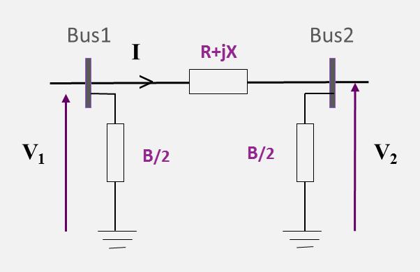
Besides, Technical losses in the distribution system are caused generally by the physical properties of the network elements (conductors, equipment used for distribution line, transformer) [4]. Theheat dissipation dueto current flowing in the electrical network created line losses, which is well known as joule effect: ���� =����2

Losses in transformer are due to iron losses and copper losses. The iron losses are caused by the cores magnetizing inductance (Foucault current and Hysteresis) that dissipated a power, whereas Copper losses are by the winding impedance inside the transformer.

Inotherwords,thetechnicallosses resultfromtheactive andreactivepowerflowinthenetwork.Activepowerlosses are due to the over loading of lines characterized by the resistance. Low voltages and variation of powers flows in each bus can produce also these active losses. Otherwise, reactive power losses are produced by the reactive elements (the reactance of the line).

On the one hand, total active and reactive power losses are computed with:

Where Ploss and Qloss are respectively the active andreactive power losses ; nbr is the number ofbranches of the system, Ii the current flowing through the branch, Ri the resistance of the branch iand Xi the reactance of the branch i

On the other hand, the overall active power losses of the entire network are obtained by the differencebetween the active generated power and the active consumed power.

For similar reason, the total reactive power losses of the network are equivalent to the reactive generation or consumption of the network. That is to say the sum of the reactive powers injected or absorbed by the generators is equal to the sum of reactive power consumed or generated by the load added the sum of reactive generation or consumption of the network.

III. METHODOLOGY FOR POWER LOSSES ASSESSMENT AND INFLUENCING FACTORS IDENTIFICATION

3.1 ASSESSMENT OF POWER LOSSES BY NEWTON RAPHSON METHOD

Different technics are used to assess the power losses. As we see in the expressions (3) and (4), the Global losses of the network can be deduced through these equations, in condition that all injected powers (active and reactive) and bus voltage (V,) in each bus are known. But the problem is we cannot get easily the voltage at different buses of the system because of the interdependence between the bus voltage and the different powers at load bus. The main difficulty in evaluating power losses in distribution network is the nonlinear relationship between the injections powers at the buses and their variables associated [3]. For this reason, resolutionby the power flow(Load flow)is required for a good assessment. Several methods have been used for load flow calculation such as the GAUSS-SEIDEL method, the NEWTON-RAPHSON method, the bi- factorization method of K-ZOLLENKOPF, the relaxation method, the DC-Flow method, ... Among these different methods, we prefer to use the Newton Raphson method because this method converges much faster. In addition, this method can transform the original non-linear problem into a sequence of linear problems whose solutions approach the solutions of the original problem. The solution to the power flow problem begins with identifying the known and unknown

variables in the system. These variables (P, Q, V,) are the characteristics of each bus in the network that are respectively the active power, the reactive power, the voltage magnitude and the voltage angle. These four variables are dependent on the type of bus. So, two of them must be known in each bus. If P and V are known, that means a generator is connected to the bus, it is called a Generator Bus. In contrary, if no generators are connected to the bus, it is the Load bus (or PQ Bus). Aside this, resolving load flow problem needs one bus that chosen arbitrarily and the value of the voltage (V, Ɵ) must be fixed before a program execution. This bus is known as Slackbus.

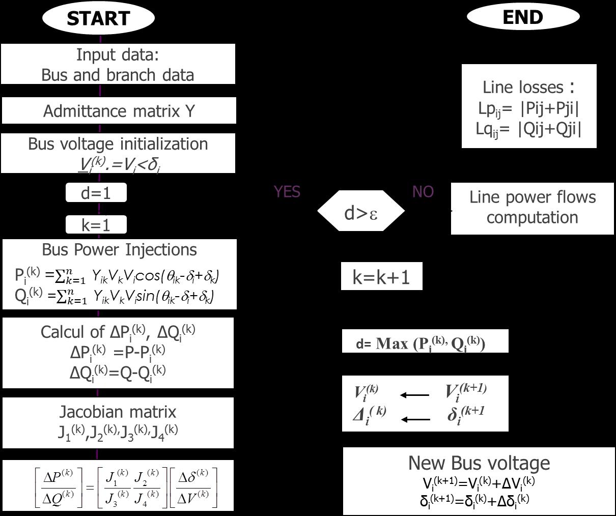
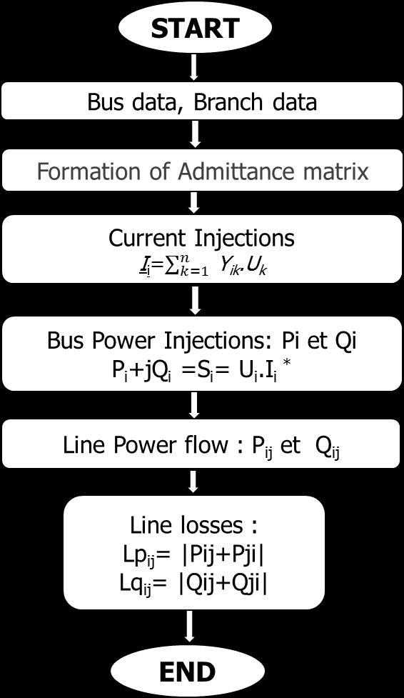
The common process of load flow computation is summarized on the organigram 1 (Fig 1) while the specificity of NRLF method [11] and its algorithm details are shown in Fig 2.

Fig. 1: Organigram of Load Flow

Fig. 2: Organigram of Newton Raphson Load Flow

3.2. SENSITIVITY ANALYSIS BY OAT METHOD

The sensitivity analysis SA is a mathematical tool that observes the output of a model in relation to the variations of different input factors and quantifies their influences on the model. According to Jolicoeur [12], it happens often a lot of parameters in a complex mathematical model, and they do not have the same degree of influence on the model outputs. Some have more important contribution than others. Thus, a sensitivity analysis can help predict the effect of each parameter on model results and classify them according to their degree of sensitivity [13]. There are mainly three different methods of SA: the Local Sensitivity Analysis (LSA), the Global Sensitivity Analysis (GSA) and the Screening Designs (SD). The using of each kind of method depends on the objectives that users want. These methods are widely described with Bertrand and al. in [14] and Kleijnen and al. in [15].

What we are interested in these methods is the “Screening Designs” (SD) which contains the “One-FactorAt-A-Time” method because it is efficient when a model has many input parameters

[12]. It has a purpose to arrange the most important factors among many others that may affect a particular output of a given model. Although OAT approach is to

assess the relative importance of input factors with uncertainty, and applied only in linear model [13], this is the reason why Newton Raphson method has been chosen to transform the non-linearity of the load flow problem into a linear application.

In this case, all the linear parameters and the bus characteristics have been contributed to the analysis, because it consists to find the effect of each parameter on active power loss in each branch.

Totally, 14 parameters are studied except the voltage angle  because it was taken automatically as zero during the bus voltage initialization (principle of slack bus).

Fig. 3: A two-bus system

Table 1: Parameters with their variation range

Qc(NE)

Consumed Reactive power in the extreme bus [0 :30] MVar

15  Voltage angle °

The relative variation rate ����(��) [16], and the sensitivity index SI(p) [12], in a parameter p of a model can be computed as these following expressions:

American Electric Power System (in the Midwestern US) as of December, 1961. The data was kindly provided by Iraj Dabbagchi of AEP and entered in IEEE Common Data Format by Rich Christie at the University of Washington in August 1993.

Where:

• E1 is the initial input parameter;

• E2 is the tested input value (: ±v% modification; “v” is a given percentage, it depends on the parameters. For the linear parameters R, X, B and the different powers; a variation of +/- 10% is acceptable. And for the bus voltage, a +/- 4% is acceptable because the variation range in p.u for voltages are between 0.90 and 1.10)

• Eavg the average between E1 and E2

• S1, S2 are respectively the outputs value corresponding to E1 and E2;

• Savg is the average between E1 and E2.

IV. RESULTS

4.1. MESHED DISTRIBUTION NETWORK IEEE-30 BUS

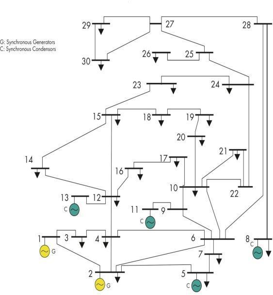
The case study is the 30 Bus Test meshed distribution network from the IEEE [18]. It represents a portion of the

This system has 30 buses, 41 branches, 2 synchronous generatorsinbus1and2thatproduce300,2MWaltogether, 4 synchronous compensators in buses 5,8,11,13 and 4 transformers 132kV/33kV in branches 11,12,15 and 36.

Fig. 4: One-line diagram of the IEEE 30bus

Table 2: Bus data of meshed network IEEE-30 BUS

Table 3: Branch data of meshed network IEEE-30 BUS

4. 2. POWER LOSSES BY NRLF

As shown in table 4, the different powers flowing in each bus are obtained. Table 4: Injected, generated and consumed powers in each bus

The results show that the sum of the injected active powers in every bus represents also the same value as the table 5 shows. That is the total active power losses in that network.

This result justifies the two ways for power losses assessment as mentioned in equation (3) and (4)

Table 5: Different power flows and losses between bus i and j

4.3. INFLUENCING FACTORS ON POWER LOSSES

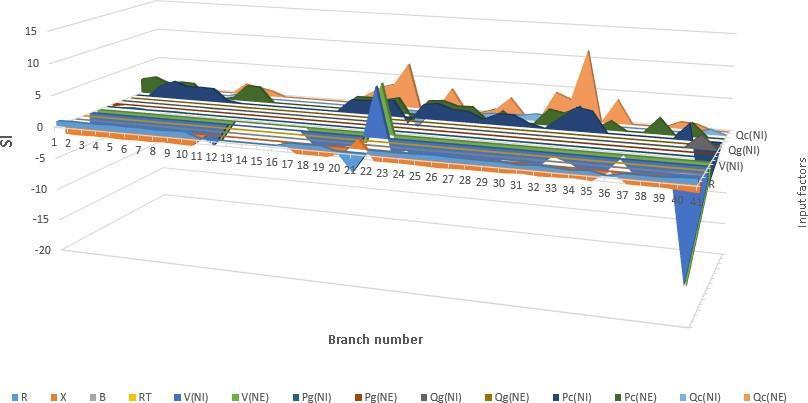
As we observed on the global representation of the Sensitivity index (Fig. 5); many high peaks have been appeared that indicate the most influencing parameter in the corresponding branch (Tables 6, 7)

A SI positive means that the variation of the inputs value is the same direction as the variation in the output whereas a SI negative represents an inverse effect between the inputs and the output factors It could be seen that each branch has its influencing factor which differs from each other.

Table 6: Sensitivity Index of the 14 parameters

Fig. 5: Global representation of the factor effect on each branch according to the SI values

Table 7: Relative variation rate of the 14 parameters

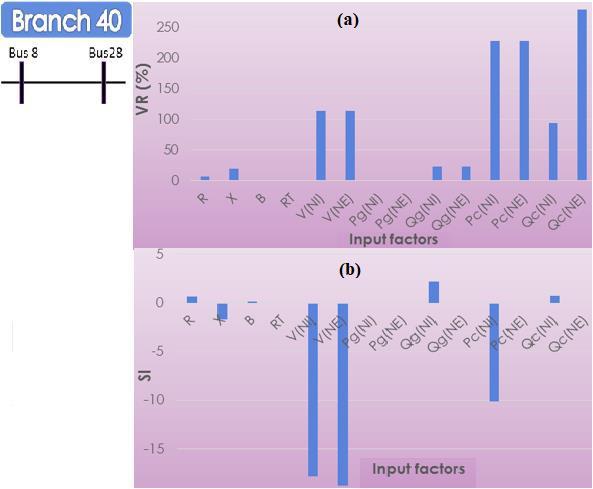
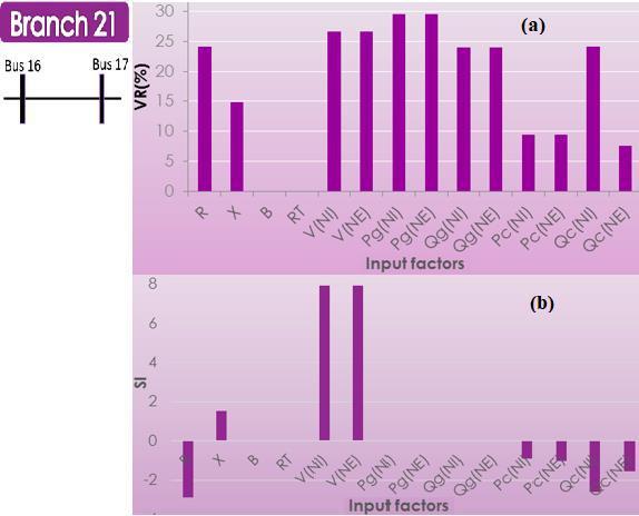
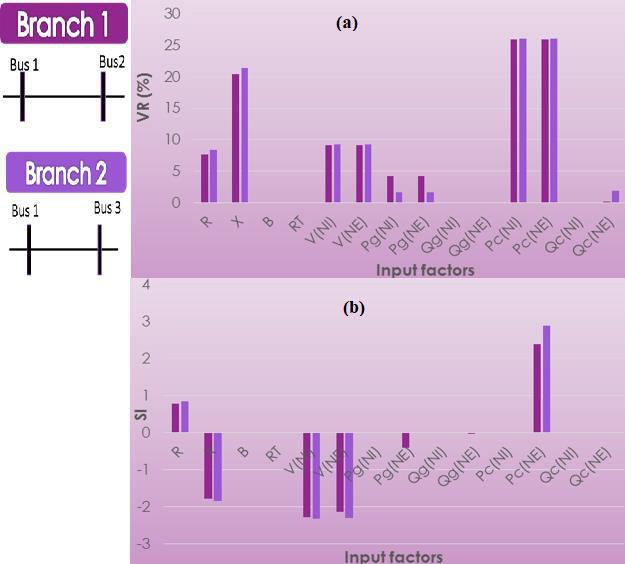
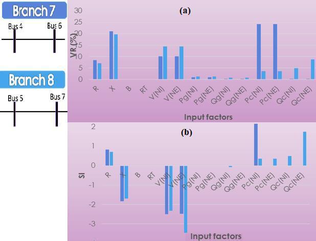
Some specific branches are presented in Fig. 6 to Fig. 9 to show the effect of the parameters through Vr and SI values.

The most highlights branches are the branch 21 and the branch 40 which are affected by the bus voltage and the reactive powers in the extreme bus.

In the first branch of which the two generators are connected to the buses, there is no effect of the reactive powers as shown in the Fig. 6 (a), (b)

Concerning the branch 21, high rate of Vr appeared in each parameter due to the variation of voltage magnitude beyond the limits. For the branch 40, Vr of the bus 28 is very high due to the effect of reactive power at the bus 8.

V. DISCUSSION

In this case by the given data from (Fig. 4),synchronous compensators are placed by network operators in buses 5, 8, 11 and 13. But according to the research of Dharamjit and al. [17], compensators are injected at the network in buses 13,22,23 and 27.

At this work, we have found that there is some issues related to voltage, generated and consumed reactive powers in buses

8,16,17 and 28. So, it will be better if any other energy sources or compensators are injected to these buses.

VI. CONCLUSION

Using NRLF method was chosen, in this work, to quickly assess the power losses on the 41 branches of the IEEE 30bus meshed distribution network. Identifying these losses with their influencing factors could help electricity distributors to find the issue of each branch in order to apply an optimization of their networks.

Among the parameters investigated of each branch during the analysis by OAT, the result shows that the most influencing parameters are:

Fig. 6: Input factors in branches 1 and 2: (a) Relative variation rate, (b) Sensitivity Index

Fig. 7: Input factors in branches 7 and 8: (a) Relative variation rate, (b) Sensitivity Index

Fig. 8: Input factors in branch 21: (a) Relative variation rate, (b) Sensitivity Index

Fig. 9: Input factors in branch 40: (a) Relative variation rate, (b) Sensitivity Index

• the consumed reactive powers;

• the bus voltages;

• and the linear parameters.

In fact, the application of OAT method also allows us to know the interdependence between the variations of bus voltage and the reactive power consumptions. Concerning the required solution to optimize these losses problems, three mains suggestions are given such as:

• the reactive power compensation by using capacitor banks for the branch which have reactive powers issues;

• the injection of energy sources into the low busvoltage, like hybrid system or renewable energy;

• the reconfiguration of the network according to the suitable loads if necessary.

Finally, the application of these proposal optimizations requires more economical and technical analysis in order to avoid excessive investment and meet demand.

REFERENCES

[1] Navani, J.P.,Sharma, N.K.andSapra, S.(2012).Technical and Non-Technical Losses in Power System and Its Economic Consequence in Indian Economy. International Journal of Electronics and Computer Science Engineering, 1,757-761.

[2] Parmar,P.,(2013).TotalLossesinPower Distributionand Transmission Lines. Technical Articles in Electrical EngineeringPortal.

[3] Mendoza, J. E., Lopez, M., Fingerhuth, S., Carvajal, F., & Zuñiga, G. (2013). Comparative study of methods for estimating technical losses in distribution systems with distributed generation. International Journal of Computers, Communications and Control, 8(3), 444-459. https://doi.org/10.15837/ijccc.2013.3.470

[4] Mufutau,W.O.,Jokojeje,R.A.,Idowu,O.A.Sodunke,M.A, (2015). Technical Power Losses Determination: Abeokuta, Ogun State, Nigeria Distribution Network as a Case Study

IOSR Journal of Electrical and Electronics Engineering (IOSR-JEEE). e-ISSN: 2278-1676, p-ISSN: 2320-3331, Volume 10, Issue 6 Ver. I (Nov – Dec. 2015), PP 01-10, www.iosrjournals.org

[5] Antmann,P.,(2009).ReducingTechnicalandNon-Technical LossesinthePowerSector.©WorldBank,Washington,DC. https://openknowledge.worldbank.org/entities/publication/7 0bb9d7e-1249-58aa-bc54-ee9f2cfb66cf.

[6] Ramesh L., Chowdhury S.P.C., Natarajan,A.A., Gaunt C.T., (2009).MinimizationofPowerLossindistributionnetworks by different techniques World International Journal of Scientific&EngineeringResearch.

[7] Abdelmalek, G., (2010). Utilisation des méthodes d'optimisations métaheuristiques pour la résolution du

problème de répartition optimale des puissances dans les réseaux électriques. Master, Centre Universitaire d'El-oued, InstitutdeSciencesetTechnologie.

[8] Liva, GR., Mihai, G., Ovidiu, I, (2012). Multiobjective Optimization of Capacitor Banks Placement in Distribution Networks. Latest Advances in Information Science, Circuits andSystems.

[9] Madeiro S., (2011). Simultaneous capacitor placement and reconfigurationforlossreductionindistributionnetworksby a hybrid genetic algorithm. IEEE Congress on Evolutionary Computation(CEC).DOI:10.1109/CEC.2011.5949884.

[10]Nourai A., Kogan V.I., Schafer C. M., (2008). Load Leveling Reduces T&D Line losses. IEEE Transactions on PowerDelivery.DOI:10.1109/TPWRD.2008.921128.

[11]Mork,B.,(2000).NRLFformulation.EE5200

[12]Jolicoeur, (2002). Screening designs sensitivity of nitrate leaching model (ANIMO) using a one-at-a-time method. Binghampton:StateUniversityofNewYork.

[13]Saltelli, A., et al., (2006). Sensitivity analysis practices: Strategiesformodel-basedinference.ReliabilityEngineering & System Safety, Volume 91, Issues 10–11, October–November 2006, Pages 1109-1125. https://doi.org/10.1016/j.ress.2005.11.014.

[14]IoossB., LemaîtreP.,(2015). Areviewon global sensitivity analysis methods. HAL, Springer, 2015. DOI: 10.1007/9781-4899-7547-8_5.

[15]Kleijnen, J.P.C., (1997) Sensitivity analysis and related analyses Journal of Statistical Computation and Simulation, 57(1-4), 111-142. DOI: 10.1080/00949659708811805.

[16]DT., F.-M., (1990). A sensitivity analysis of Erosion/ProductivityImpactCalculatorinSharpley.

[17] Dharamjit,TantiD.K.,(2018).LoadFlowAnalysisonIEEE 30 bus System. International Journal of Scientific and Research Publications 2(11) (ISSN: 2250-3153). http://www.ijsrp.org/research-paper-1112.php?rp=P11375.

[18] http://www.ee.washington.edu/research/pstca, retrieved on June2013