9)A new Carbon Budget at a Glance

«The carbon dioxide in the atmosphere is strongly coupled with other carbon reservoirs in the biosphere, vegetation and top-soil, which are as large or larger. It is misleading to consider only the atmosphere and ocean, as the climate models do, and ignore the other reservoirs. Fifth, the biological effects of CO2 in the atmosphere are beneficial, both to food crops and to natural vegetation. The biological effects are better known and probably more important than the climatic effects.» Freeman Dyson

From all what has been seen in this first Chapter, a very different Carbon Budget from what is proposed by IPCC can be suggested, where the various notions seen can be put together. The amount of carbon dioxide in the air is a consequence of the surface temperatures of the inter-tropical zone where most of the ocean degassing takes place (Figure 10). 94% of the carbon dioxide in the air comes from the natural degassing of the oceans (Levy et al., 2013) and is the time integral of past temperatures (Figure 8, Equation 23), a consequence of these temperatures (Equations 18 and 19), and therefore cannot be the cause. Only 6% of the CO 2 in the air is what remains from fossil fuels after that a fast circulation with the oceans happens (Equations 6 and 16). A simple polytropic relationship between temperature and pressure describes the air and surface temperatures (Equations 60 and 61). Water vapor makes the Earth's atmosphere extremely opaque over the bulk of the thermal infrared spectrum (Figures 13, 15, 16), Table p. 59 after Equation 69, and Equations 70, 71: the atmosphere cannot, at these frequencies, transport heat by radiative mechanisms; the surface loses the heat received from the sun mainly by evaporation and convection. The thermal infrared radiation of the troposphere, 80% of that of the globe, is regulated and controlled by the water vapor content of the air around 300 millibar (9 km) (Figures 19, 20, 21); changes in the carbon dioxide content of the air cannot have an effect because the water vapor content of the upper troposphere is extremely dynamic and quickly adjusts the thermal infrared radiation to the solar heat absorbed under the tropopause.

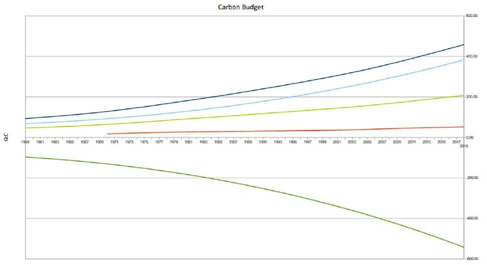
Figure 28. Carbon Budget at a glance over the period 1900-2018 displayed on the graph over 1959-2018. Dark Blue = Cumulated man-made emissions Gt-C (same as Figure 5), Light Blue= Cumulated Degassing by the Oceans yr-1 of Total Gt-C in Atmosphere, Light Green = Cumulated Gt-C Budget (overall ppm atmospheric increase), Red = Anthropic Gt-C CO 2 remaining (same as Figure 5), Green = Cumulated uptake by Land, Forest, and Biological Punp yr -1 of total Gt-C in Atmosphere. Based on a non linear model where all processes are dependent on the Temperature.

The Carbon budget (CB) proposed (1900-2018) illustrated by Figure 28, takes into consideration what has just been reminded here. Let's see how it has been computed starting from the bottom of the graph, the green curve, soils and vegetation to which can be added the Biological Pump (BP) mainly relying on the marine autotrophs (Burd et al., 2010; Passow and Carlson, 2012; Herndl and Reinthaler, 2013; Le Moigne, 2019). Notice though that the amount accounted for by the meso and bathypelagic biological pump activity remains conjectural. This series, the uptake by the soils and vegetation (Usv+), is obviously proportional to the total amount in Gt-C of CO 2 in the atmosphere which as explained above is dependent on the temperature and results from it. In fact, the reason is that the Primary Productivity (PP) of

the autotrophs depends on both. The coefficient αsv (-0.017) will characterize the uptake by the soils and vegetation (negative as it corresponds to an uptake) and the βi will be an arithmetic progression of common difference of 0.013 to model the progressive increase of the uptake as the temperature progresses and the total atmospheric [CO 2] in ppm does the same. The initial β0 equals 0.2. This model as represented by Equation 156, leads to an uptake by soils and vegetation of 571,52 Gt-C over the period (1900-2018) and the increased primary production of the autotrophs is what has driven the uptake and growth of that sink from 1900 to 2500 Gt-C (Campbell et al., 2017; Haverd et al., 2020), somehow 600 Gt-C.

n

Usv n

= β 0 α sv Usv0+∑

i=1 β i α sv Usv i with β 0 =0.2 ; βi = βi-1+0.013 ; α sv =−0.017 (156)

The second time series in Red is what is left of the anthropogenic emissions after n=118 years, i.e. 52.15 Gt-C as resulting from Equation (6).

The light-green curve corresponds to the CB itself, the cumulated sum of the yearly anthropogenic emissions, minus the fraction removed, minus the uptake by soils and vegetation, plus the degassing from the oceans. As an indication, for 2018, man-made emissions (+10.15 Gt-C), minus fraction removed (-1.82 Gt-C), minus net uptake by soils and vegetation (-14.48 Gt-C), plus net degassing by the oceans (+10.22 Gt-C), leads to an overall Gt-C Budget (+4.05 Gt-C). This positive number should be reduced by increased DOC and POC due to the increased primary productivity of the oceans, but are hard to assess accurately, e.g. Toggweiler (1990) p. 122 states “ Druffel and Williams112 now add new evidence that supports the dissolved organic pathway. They have measured the degree to which the 14C produced by nuclear weapons testing has contaminated the particulate organic carbon (POC) pools, both sinking and suspended, in the North Pacific. At present, inorganic CO2 in the water below the upper kilometre of the ocean is uncontaminated with respect to bomb 14C. This is not true, however, with respect to the organic carbon in particles. Large settling particles can sink to the bottom in less than a year”. So, this number is a “worst case” figure. The light-green curve is the total cumulated CB over the period 1900-2018.

The light-blue curve represents the total cumulative degassing of the oceans over the period 1900-2018. It is computed according to the same logic as the uptake by soils and vegetation except that we consider a positive contribution to the CB as the degassing (Docean) is dependent on the temperature, which as it progresses leads to more out-gassing. The same approach as for Equation (156) is used, except that the αocean (+0.012) is positive (net contributor to the CB). Overall, the process is calculated in the following way:

n

Docean n = β0 α ocean Docean0+∑

i=1 β i α ocean Doceani with β0 =0.2 ; βi = β i-1+0.013 ; α ocean =+0.012 (157)

During the same period, also driven by the temperatures, the oceans have net out-gassed in this model 403 Gt-C, given the fact that the solubility of CO2 in seawater has globally slightly decreased as per Henry's law. Overall, in the picture presented, the atmosphere has had an increase of approximately 200 Gt-C as the net result of all these processes.

The dark blue curve represents the cumulated man-made emissions in Gt-C over 1900-2018 and amount to 458 Gt-C.

The way the land, forests and vegetation and BP uptake and the oceans net degassing have been represented rely on a non-linear model (βi times αsv or times αocean) that depends on the temperature and which progressively increases the net degassing by the oceans and the uptake by soils and vegetation as T goes up (and reversely goes down) according to a simple “peg” to the total atmospheric [CO2] in Gt-C and an arithmetic progression. All processes end up with a consistent overall atmospheric CO2 ppm increase of approximately 200 Gt-C which matches well what was observed of 209.80 Gt-C.

One should not be mistaken by the appearance of high accuracy of the numbers given above. They are just reasonable gross estimates that demonstrate that a CB can be balanced on completely different hypothesis than those adopted by IPCC e.g. (Le Quéré et al., 2016, 2018); but obviously nobody knows whether over the timescales 1900-2018 the vegetation has had an uptake of -600 Gt-C or as calculated here of -571.52 Gt-C or whether the oceans have degassed +403.42 or simply +352 Gt-C as evaluated by means of Equation (9) p.29, etc. What should be remembered is that

112(Druffel et al., 1992)

fundamental physical and chemical processes are operating before us and that first and foremost these should be accounted for: the soils and vegetation act as a sink, the oceans ensure a fast circulation with a large reservoir leading to a short residence time for any CO2 molecule in the atmosphere of less than five years and even though they ensure the removal of some DIC, DOC and POC by deep precipitation, they globally degas as the temperature has increased since the end of LIA and that should be reflected in any decent CB.

What remains of the 458 Gt-C of total anthropogenic emissions is a small fraction of just 52.15 Gt-C and the overall 210 Gt-C increase of the CO2 atmospheric stock has a complex explanation (balancing all sources and sinks) and does not mainly result of the man-made emissions113, a preposterous hypothesis made by IPCC authors. Schimel et al. (2015) rightfully reminds that “Feedbacks from terrestrial ecosystems to atmospheric CO2 concentrations contribute the second-largest uncertainty to projections of future climate. These feedbacks, acting over huge regions and long periods of time, are extraordinarily difficult to observe and quantify directly.”

The CB presented here that focuses on natural phenomenons, which are by far of a greater order of magnitude than the total of the man-made contributions, and most probably underestimates the role of the oceans into sequestering part of the organic carbon that it contains, especially given the fact that the increased oceanic productivity which goes along with an increase of the temperature and of the availability of CO 2 lead to more organic sequestration. As Steele (2020) summarizes “Productivity increased after the last glacial maximum ended, and increasing organic sediments on the sea floor suggest increased carbon sequestration”. So even though the oceans are net degassing for obvious physico-chemical reasons, their uptake of organic and particulate organic matter are underestimated in the aforepresented Carbon Budget, but one can hardly assess objectively to how much these additional sinks amount by now.

In fact, the IPCC Carbon Budget does not stand the quickest scrutiny. As per IPCC, CO 2 emitted by fossil fuel consumption can only find its way into three different sinks: accumulate in the atmosphere, be dissolved and removed by the oceans or finally be absorbed by the vegetation or the phyto-plankton that it feeds. This is represented graphically by the Figure 6.8, p. 487 of IPCC (2013) and shows large yearly variations from -0.5 to +4 Gt-C. It is worth noticing that only the atmospheric part of such a budget is measured, by means of IR spectrometry, whereas the other components are either the result of a model (ocean uptake) or of a simple subtraction from the two previous numbers. As such, by way of just obtaining the land uptake by that subtraction, this value appears as the simple “negative” of the annual atmospheric variations.

As per the IPCC CB, the uptake by the vegetation would have been minimum, in fact even negative, the warm El Niño years like 1983 (2.57 ppm increase) with -0.3Gt-C and 1998 (3.28 ppm increase) -0.5 Gt-C, whereas the uptake by vegetation would have been maximum with values of 4Gt-C in 1992-93 (ppm increase of [1.01-0.5]), much colder years, by around 1°C, than 1998. Thus, as per IPCC carbon budget, during warm years the vegetation would appear unable to capture any CO2 at all, with even negative numbers, letting the emissions accumulate as per their model in the air and the oceans, whereas the maximum uptake would happen during cold years. Such a curious model is defeated by the obvious observation of the Keeling curve that shows that the seasonal variations of the [CO 2] is mainly due to its consumption by the vegetation. It shows that there does not exists the kind of difference that appears in the IPCC budget [-0.5-4]Gt-C, the curve being very repetitive from one year to the next, displaying comparable patterns of seasonal variations and showing for the years 1992-1993 or 1998 comparable vegetation consumption during spring and summer of 17 Gt-C. One immediately sees the absurdity of such IPCC CB model as if the vegetation was unable to provide for any uptake the warm years, why the UN would undertake massive tree planting operations, that despoil peasants in countries like Uganda and Cameroon? The conclusion is that the IPCC carbon budget shows an entirely erroneous behavior for the land and vegetation sink as a result of considering it as a simple subtraction of the two other sinks.

113This is of course a very different approach to that of the Le Quéré et al. (2016) paper which necessitated 68 authors (argument of authority ?) to come up with an IPCC compliant CB which leaves no place to Nature. These Le Quéré et al. (2016, 2018) CBs are based on the combination of a range of data, algorithms, statistics, and model estimates and their arbitrary interpretation by a broad and partisan community tainted by major conflicts of interest because their economic and social survival depends on continued state funding based on the erroneous assumption that CO2 only results from anthropogenic emissions. The global carbon budget of all these researchers, ensconced in the comfort of their laboratories, asserts that averaged over the decade (2006–2015), 91% of the total emissions were caused by fossil fuels and industry, and 9% by land-use change. Nothing from

Nature; this is meaningless. So many authors were required to impress the reader, make him/her believe that Nature has no role to play and come up with sort of a dogma based on a dubious interpretation of data and on gimmicked models; what an outlandish and ludicrous claim to think that these arbitrary guesstimates bear any resemblance to reality and would justify coercive economic policies to be based on them.

The approach and the model presented here is certainly not settled, nothing is never, and will be improved and refined as our understanding progresses but it has the merit of giving reasonable and rational orders of magnitude for the physical, chemical and biological processes that any objective observer and scientist must first and foremost account for; e.g. Henry's law and the degassing of the oceans cannot be ignored and is obviously one of the main players of the CB budget. Never ever any honest scientist should start from foregone conclusions and try to thwart the reality in so far as to make it match the flawed assumptions (i.e. man-made emissions are 100% responsible of the CO2 increase and for sure, Nature does not play any role), only pseudoscience does that. Science works the other way round, but IPCC has corrupted it by supporting and funding only the dogma that man-made emissions were responsible of everything, nothing to argue about, science is settled ; this will prove ultimately extremely detrimental to the confidence that the public will place in science in the future when the dogma will unravel as a card castle facing the climate reality, that will not conform to the AGW lunacies and forecasts.

As a brief summary, not only does CO2 have a very little effect as the atmosphere is very opaque to IR radiations (e.g. Equation 80 and corresponding Table), but its radiative contribution is very small even considering the water vapor feedback (Equations 81, 82)114, and in the end most of the heat distribution which makes the climate is related to other processes such as transport by latent heat (i.e. evaporation – condensation – precipitation), sensible heat (i.e. convection – advection), etc., or radiation by the TOA where the regulation by water vapor is far more important than any role that CO2 could play, but furthermore one must acknowledge that most of its increase (210 Gt-C) since 1900 is

not even of anthropogenic origin!

114Even as per the flawed IPCC model based on SBL, CO2 delivers a muted log-response (Equations 83, 84) which had to be reinforced arbitrarily by a number of nonsensical hypothesis in order to make it have some climatic impact!