Nature Controls the CO2 Increase - EB

Vol. 3.1 (2023)

pp. 68-91

Nature Controls the CO2 Increase

Edwin X Berry

Ed Berry LLC, Bigfork, Montana 59911, USA

Abstract

Climate alarmism and politics are based on the invalid United Nations (UN) assumption that human CO2 is the dominant cause of the CO2 increase above 280 ppm, or since 1750. This assumption conflicts with UN’s own data, is derived from invalid circular reasoning, and violates physics. UN data show human carbon emissions have added only 33 ppm to atmospheric CO2 as of 2020 while natural CO2 emissions added 100 ppm. This predicted human-caused increase of 33 ppm is 8% of the total carbon in the atmosphere as of 2020, not 33% as the invalid assumption claims..

Also, δ14C data prove nature is the overwhelming cause of the CO2 increase since 1750, and lower the 8% of human carbon in the atmosphere calculated from the UN data to less than 4 percent. The relative equilibrium percentage levels of available natural carbon in land, air, surface ocean, and deep ocean is the strongest predictor of the effect of human carbon on atmospheric CO2 because the independent human carbon cycle seeks the same percentage levels as the equilibrium natural carbon cycle. For example, if the carbon levels of land, surface ocean, and deep ocean were each doubled, the effect of human carbon emissions on atmospheric CO2 would be reduced by about half, to 18 ppm.

The bomb-caused increase in 14C and δ14C has now depleted as δ14C has returned to its balance level of zero. Yet the 14C level is now higher than in 1950. To explain this 14C increase, we propose a theory that nature keeps the δ14C balance level equal to zero. This theory predicts the non-bomb 14C increase since 1950 is caused by the 12C increase while the δ14C balance level stayed at zero. This is the simplest (Occam’s Razor) explanation for the non-bomb 14C increase since 1950.

Keywords: CO2; carbon cycle; climate change; climate emergency; climate alarmism; climate fraud; climate crisis; human emissions.

Submitted 15-02-2023. Revised version 20-03-2023. Accepted 21-03-2023.

https://doi.org/10.53234/scc202301/21

1. Introduction

The Intergovernmental Panel on Climate Change (IPCC, 2013, p. 467, Executive Summary, selected paragraphs) say incorrectly and without scientific basis,

The Human-Caused Perturbation in the Industrial Era CO2 increased by 40% from 278 ppm about 1750 to 390.5 ppm in 2011.

With a very-high-level of confidence, the increase in CO2 emissions from fossil fuel burning and those arising from land use change are the dominant cause of the observed increase in atmospheric CO2 concentration.

About half of the emissions remained in the atmosphere (240 ± 10 PgC) since 1750.

It is virtually certain that the increased storage of carbon by the ocean will increase acidification in the future, continuing the observed trends of the past decades.

The removal of human-emitted CO2 from the atmosphere by natural processes will take a

Edwin X Berry: Nature controls the CO2 increase

few hundred thousand years (high confidence).

… about 15 to 40% of emitted CO2 will remain in the atmosphere longer than 1,000 years. This very-long time required by sinks to remove anthropogenic CO2 makes climate change caused by elevated CO2 irreversible on a human time scale.

By contrast, since the beginning of the Industrial Era, fossil fuel extraction from geological reservoirs, and their combustion, has resulted in the transfer of significant amount of fossil carbon from the slow domain into the fast domain, thus causing an unprecedented, major human-induced perturbation in the carbon cycle.

IPCC’s first sentence above defines what we call IPCC Theory (1), which says that human CO2 is the overwhelming cause of the measured CO2 increase since 1750, when according to the IPCC the CO2 level was 278 ppm, or approximately 280 ppm.

According to the IPCC, the natural CO2 level remained at about 280 ppm since 1750.

Berry (2021) used IPCC’s own natural carbon cycle data to compute IPCC’s true human carbon cycle, which shows that nature, not human CO2 emissions, drives the CO2 increase. So, while the IPCC claims “with a very-high-level of confidence” that human CO2 emissions caused the CO2 increase, IPCC’s own data say with a very-high-level of confidence that natural CO2 caused the CO2 increase.

Thus, IPCC’s own data prove its Theory (1) is false. This conclusion cannot be ignored. According to the scientific method, data prevails over theory and over votes by scientists. Therefore, Berry’s (2021) proof that IPCC’s Theory (1) is false based on IPCC’s own data is the new default truth that must be proved wrong before anyone can legitimately claim or believe that Theory (1) is true.

Using a different method, Harde and Salby (2021) and Harde (2019, 2017) also prove IPCC’s Theory (1) is false. These proofs that Theory (1) is false undermine IPCC’s claims about humancaused climate change. Murry Salby passed away in 2022, leaving Hermann Harde to support and defend their proofs that the IPCC Theory (1) is false.

Salby and Harde (2022) is a research masterpiece that shows how increasing temperatures are the true cause of increasing CO2.

Science progresses when we prove theories are wrong. A correct prediction does not prove a theory is true, but one bad prediction proves a theory is false. That is the key to science.

2. This is the first open debate of Theory (1)

Andrews (2023) is the first formal public challenge to Berry (2021). Andrews represents all scientists who still claim Theory (1) is true. He stands for scientists in the IPCC, America’s National Academy of Scientists (Pickering, 2016), the American Meteorological Society, American Physical Society, and in universities from the University of Montana to MIT and Caltech who still incorrectly assume Theory (1) is true. Andrews also stands for the Heartland Institute and the CO2 Coalition (Burton and Wrightstone, 2022) whose scientists make the same invalid claims and errors that Andrews presents.

Andrews (2023) makes the same arguments as they do but better than they do. So, thanks to Andrews, the debate on Theory (1) is now on the table.

Andrews writes,

A cornerstone of the argument that humans are responsible for climate change is the consensus among climate scientists that human activities such as the burning of fossil fuels have caused the rise of atmospheric CO2 concentration during the Industrial Era, all of it.

This is perhaps the most well-established piece of the case for anthropogenic global warming.

Andrews (2023) says he will provide,

A simple and compelling argument that human emissions, not natural sources, have caused the increase.

However, “consensus” is not evidence, and it is fundamentally impossible to prove a theory is true. Yet, according to the scientific method, one contradiction to a theory proves the theory is false.

Top prevail, Andrews (2023) must show Berry (2021) is wrong. This paper replies to Andrews (2023) and shows how he and those he stands for make one big fundamental error that no scientist should ever make. Their argument is based on circular reasoning that even they do not recognize.

Andrews’ circular reasoning error invalidates his related criticisms of Berry (2021, 2019), Harde and Salby (2021), Schroder (2022), and Skrable et al. (2022a; 2022b) because all his criticisms derive from his overlooked invalid assumption that Theory (1) is true.

3. Physics carbon cycle model

3.1 Physics carbon cycle model supersedes IPCC’s models

This summary is a necessary reference because Andrews and others claim Berry’s physics carbon cycle model is wrong.

Berry’s (2021) physics carbon cycle model for IPCC’s carbon cycle supersedes earlier IPCC carbon cycle models in its simplicity, versatility, and accuracy. The IPCC and its authors should have used this physics model.

Berry derives his carbon cycle model for one reservoir in only 8 equations. Then he expands his single reservoir model to multiple reservoirs to simulate IPCC’s full carbon cycle. His model exactly replicates IPCC’s natural carbon cycle at equilibrium using only one simple hypothesis that the IPCC itself approves. His model can be easily expanded to more than 4 reservoirs.

Berry‘s physics model is a valid systems-engineering model where levels set outflows and flows set new levels. This is the same formulation and computational method used by Kemeny and Snell (1960) for Markov Chains, Forrester (1968) for systems models, and many systems engineering books. Berry follows Scarborough (1966) to guide his numerical integrations.

Berry used the same systems formulation and numerical methods in his PhD thesis to calculate cloud droplet growth by stochastic collection. See Berry (1967, 1969) and Berry and Reinhardt (1974a, b, c, d) which revolutionized the way scientists now calculate particle growth.

The physics model has only one hypothesis – outflow equals level divided by an outflow time (that we call “e-time”) – that the IPCC itself recommends but does not always follow. The physics model is not a curve fit, but it exactly replicates IPCC’s natural carbon cycle data. The IPCC has no carbon cycle model that makes this replication.

Segalstad (1998) noted that IPCC’s models do not allow CO2 to flow out of the atmosphere in linear proportion to the CO2 level, which means IPCC’s models are not valid. Rather, IPCC’s models use a non-linear constraint on the outflow that contradicts physics and chemistry.

IPCC’s human carbon cycle models incorrectly assume Theory (1) is true. They use Greens functions to solve core equations, and pulse additions of Greens functions to do annual sums, a method that is not as simple, efficient, and correct as Berry’s numerical calculations.

3.2 Berry’s physics model for one reservoir

We follow Berry (2019, 2021) for the derivation of the physics model.

Fig. 1 shows the one-level physics model with one inflow and one outflow.

Inflow sets the balance level. Level sets the outflow. Level always moves toward its balance level. The outflow time, or e-time, is set by the data.

Inflow sets the balance level. Level sets the outflow. Level always moves toward its balance level. The outflow time, or e-time, is set by the data.

The physics model derivation begins with the continuity equation (1) that says the rate of change of level is the difference between inflow and outflow,

dL / dt = Inflow – Outflow (1)

where

L = carbon level (PgC)

t = time (years)

dL / dt = rate of change of L (PgC / year)

Inflow = carbon inflow (PgC / year)

Outflow = carbon outflow (PgC / year)

When Outflow = Inflow, then dL/dt = 0. The flows continue while the level is constant. The physics model has only one hypothesis, outflow is proportional to level,

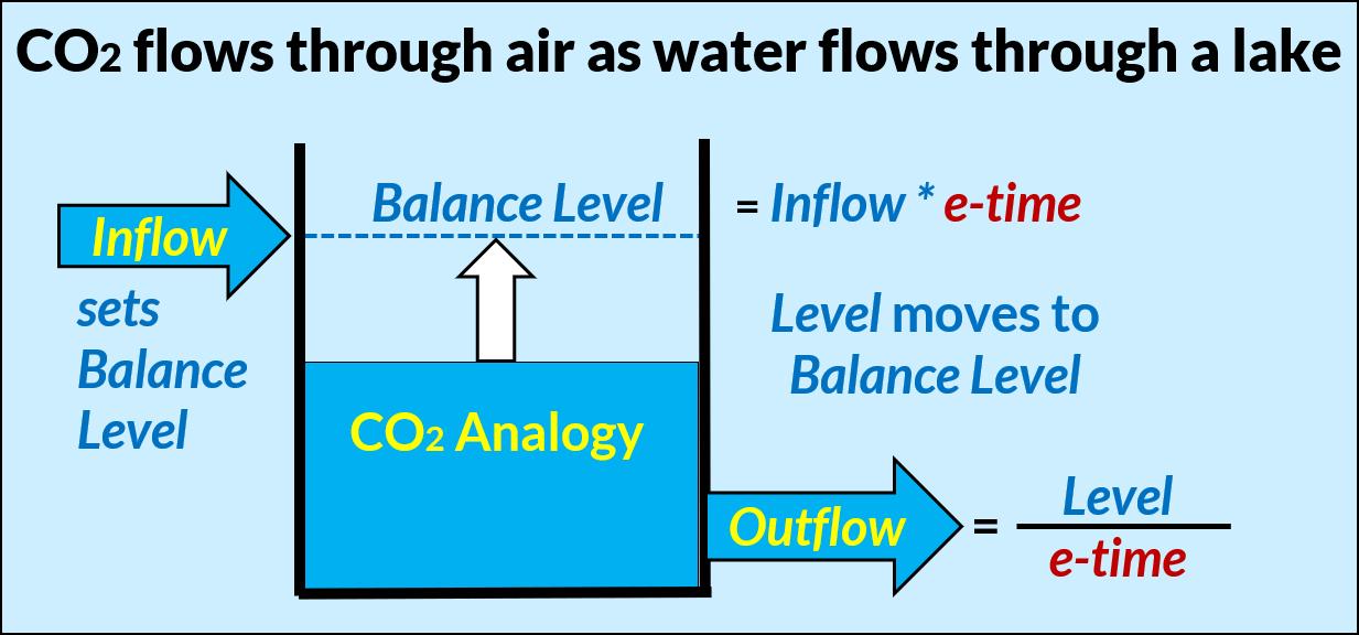
Outflow = L / Te (2)

where Te is the “e-time,” so defined because it is an exponential time. Equation (2) shows e-time Te is the same as IPCC’s turnover time, T

e-time is the time for the level to move (1 - 1/e) of the distance from its present level to its balance level.

Substituting (2) into (1) we get,

dL / dt = Inflow – L / Te (3)

When dL/dt is zero, the level will be at its balance level, Lb, defined as,

Lb = Inflow Te (4)

Substitute (4) for Inflow into (3) to get,

dL / dt = – (L – Lb) / Te (5)

Equation (4) shows how inflow sets the balance level. Equation (5) shows the level always moves toward the balance level set by the inflow. The variables L, Lb, and Te are functions of time.

Figure 1. The physics model for one inflow and one outflow node.

Edwin X Berry: Nature controls the CO2 increase

In the special case when Lb and Te are constant, which means Inflow is constant according to (4), there is an analytic solution to (5). Rearrange (5) to get,

dL / (L – Lb) = – dt / Te (6)

Then integrate (6) from L0 to L on the left side, and from 0 to t on the right side to get,

ln [(L – Lb) / (L0 – Lb)] = – t / Te (7)

where

L0 = Level at time zero (t = 0)

Lb = the balance level for a given inflow and Te

Te = time for L to move (1 – 1/e) from L to Lb

e = 2.7183

We define half-life, Th, as the time for the level to fall to half its original level. Then (7) becomes, ln (1/2) = – Th / Te (7a)

Th = Te Ln (2) = 0.6931 Te (7b)

The original integration of (6) has two absolute values, but they cancel each other because both L and L0 are always either above or below Lb

Raise e to the power of each side of (7), to get the level as a function of time,

L(t) = Lb + (L0 – Lb) exp(– t / Te) (8)

Equation (8) is the analytic solution of (5) when Lb and Te are constant.

All equations after (2) are deductions from hypothesis (2) and the continuity equation (1). There are no more assumptions and no curve fits.

IPCC (2007, p. 948) defines turnover time to equal our e-time, Turnover time (T) is the ratio of the mass M of a reservoir (e.g., a gaseous compound in the atmosphere) and the total rate of removal S from the reservoir: T = M / S. For each removal process, separate turnover times can be defined.

IPCC’s turnover time, equal to our e-time, sets how fast carbon flows out of the atmosphere. The same formula, with different e-times, applies to carbon flows out of Land, Surface Ocean, and Deep Ocean.

3.3 Physics model properties

Because (2) is a linear function of level, the physics model applies independently and in total to human and natural carbon and to all definitions of carbon or CO2. It applies independently to human CO2, natural CO2, and to 12CO2, 13CO2, and 14CO2, and their sums.

This superposition principle applies to all linear systems. The net response caused by two or more stimuli is the sum of the responses caused by each stimulus individually. So, if input A produces response X and input B produces response Y then input (A + B) produces response (X + Y).

Dalton's law of partial pressures applies to a linear system. It says the total pressure in a mixture of non-reacting gases equals the sum of the partial pressures of the individual gases.

Equation (2) is compatible with all applicable physical and chemical laws. It is the simplest hypothesis for carbon cycle models and it exactly replicates IPCC’s natural carbon cycle.

Fig. 2 illustrates how level moves toward its balance level following (8).

https://doi.org/10.53234/scc202301/21

Figure 2. Inflow sets the balance level. The level always moves to its balance level. If Inflow is constant, the balance level stays constant. There is no accumulation.

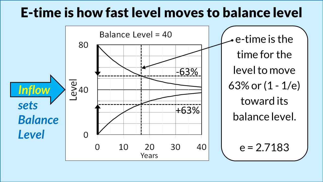
Systems models calculate outflows as functions of the levels and update the levels according to the inflows and outflows. Talk of uptakes is irrelevant because uptakes are not functions of levels. Equation (4) shows how inflow sets the balance level. Equation (5) shows how the level moves to its balance level with a speed set by the e-time. When the level equals its balance level, outflow will equal inflow and the level will remain constant.

3.4 Physics carbon-cycle model formulation

We follow Berry (2021) for the derivation of the physics model for multiple reservoirs. A popular version of this subject is in Berry (2020). IPCC’s (2013) carbon cycle has four key carbon reservoirs, e.g., land, atmosphere, surface ocean, and deep ocean.

Fig. 3 shows the physics carbon cycle model with IPCC’s four reservoirs and six outflows, where the arrows are all positive numbers. The “level” of each reservoir is the mass of carbon in each reservoir. The origin of each arrow is a “node.”

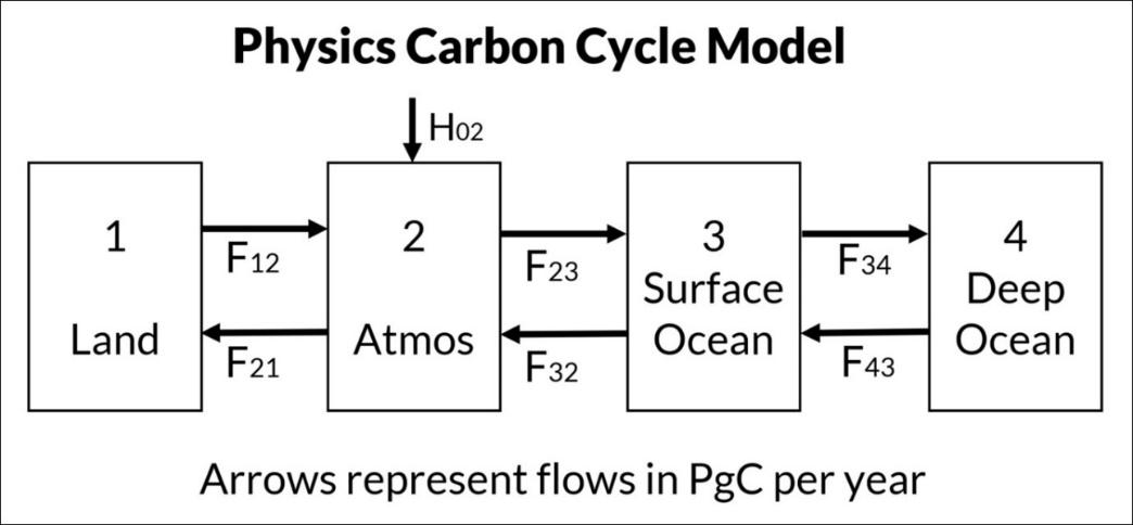
The physics model is a dynamic flow model that accurately computes the evolution of beginning levels and flows as functions of time.

Define the Levels,

L1 = level of carbon in the land

Figure 3. The physics carbon cycle model for IPCC’s carbon cycles.

Edwin X Berry: Nature controls the CO2 increase

L2 = level of carbon in the atmosphere

L3 = level of carbon in the surface ocean

L4 = level of carbon in the deep ocean

Define the individual flows out of the six nodes,

F12 = flow from land to atmosphere

F21 = flow from atmosphere to land

F23 = flow from atmosphere to surface ocean

F32 = flow from surface ocean to atmosphere

F34 = flow from surface ocean to deep ocean

F43 = flow from deep ocean to surface ocean

Define other variables,

t = time in years

H02 = human carbon flow to atmosphere

H12 = land carbon flow to atmosphere

Using (2), the flows out of the six nodes are,

F12 = L1 / T12

F21 = L2 / T21

F23 = L2 / T23

F32 = L3 / T32

F34 = L3 / T34

F43 = L4 / T43

Using (1) and (9), the rate equations for each reservoir are,

dL1 / dt = F21 – F12 – H12

dL2 / dt= F12 – F21 + F32 – F23 + H02 + H12

dL3 / dt = F23 – F32 + F43 – F34

dL4 / dt = F34 – F43

The physics model uses (9) and (10) to calculate the natural and the human carbon cycles. Numerical calculations use time steps as follows,

1. Set initial levels.

2. Calculate nodal flows using (9).

3. Calculate level rates of change using (10).

4. Multiply level rates of change by time step to get changes of levels.

5. Add changes of levels to the levels to get new levels.

6. Repeat for next time step.

(9)

Berry (2021) shows more of the computational process and supplies an Excel download showing all Berry’s calculations.

Edwin X Berry: Nature controls the CO2 increase

3.5 IPCC’s natural and human carbon cycles

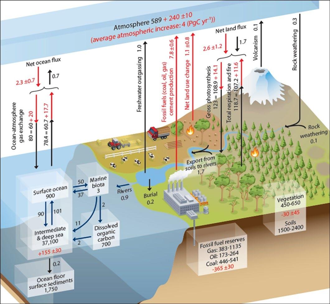
Fig. 4 is IPCC’s Figure 6.1 (IPCC, 2013, p. 471, Fig. 6.1). Fig. 4 assumes Theory (1) is true. The natural carbon level in the atmosphere stayed constant at its assumed 1750 level of 589 PgC (278 ppmv) while human carbon caused all the carbon increase above 589 PgC.

This human carbon is 29% (= 240/829) of the carbon in the atmosphere as of about 2010. By 2020, the human percentage increases to 33% (Berry, 2021).

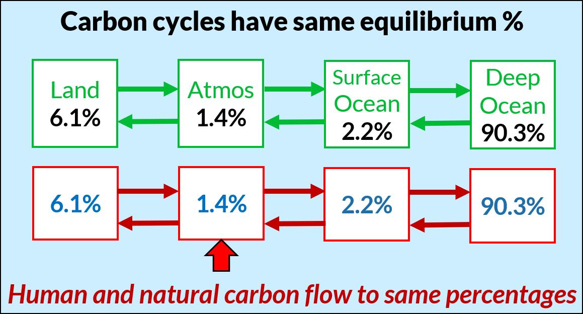
Fig. 5 shows IPCC’s natural and human carbon cycles at equilibrium. Outflow from all nodes follows (2).

The percentages in each box show the percent of total carbon in each reservoir when IPCC’s natural carbon cycle is at equilibrium. Because human and natural carbon atoms are identical, the human carbon cycle has the same equilibrium percentages and e-times as the natural carbon cycle.

Total human carbon emissions as of 2020 added about one percent to the carbon in the natural carbon cycle. So, if we stopped human carbon emissions in 2020, the equilibrium addition of human carbon to the atmosphere would be about one percent of the total carbon in the 2020 atmosphere, or about 4 ppm.

Figure 4. IPCC’s Figure 6.1 (IPCC, 2013, p. 471, Fig. 6.1) showing IPCC’s data for its shows IPCC’s natural carbon cycle (in black) and human carbon cycle (in red) as of about 2010.

IPCC’s true human carbon cycle shows nature added about three times more carbon than human carbon to the carbon cycle since 1750. So, human carbon is NOT “causing an unprecedented, major human-induced perturbation in the carbon cycle” as IPCC (2013) claims.

3.6 How to calculate IPCC’s true human carbon cycle

IPCC’s natural carbon cycle is based on IPCC’s data, which may be the best data we have for the natural carbon cycle. But IPCC’s human carbon cycle is based on Theory (1) and not upon IPCC’s natural carbon cycle data.

Berry’s (2021) insight was that IPCC’s natural carbon cycle at equilibrium has the level and outflow data necessary to calculate the e-times for each node, and these e-times apply equally to human and natural carbon. So, Berry (2021) uses data from IPCC’s natural carbon cycle to calculate IPCC’s true human carbon cycle (yellow boxes).

IPCC’s natural carbon cycle includes data, but IPCC’s Theory (1) human carbon cycle has no data. So, Berry used IPCC’s natural carbon cycle data to calculate IPCC’s true human carbon cycle.

Berry did what the IPCC should have done. He used IPCC’s natural carbon cycle data to calculate IPCC’s true human carbon cycle. The calculation is deductive, confirmed, and not complicated.

IPCC’s failure to properly calculate its true human carbon cycle has caused false climate alarmism, its costs, and failures to educate students in true physics.

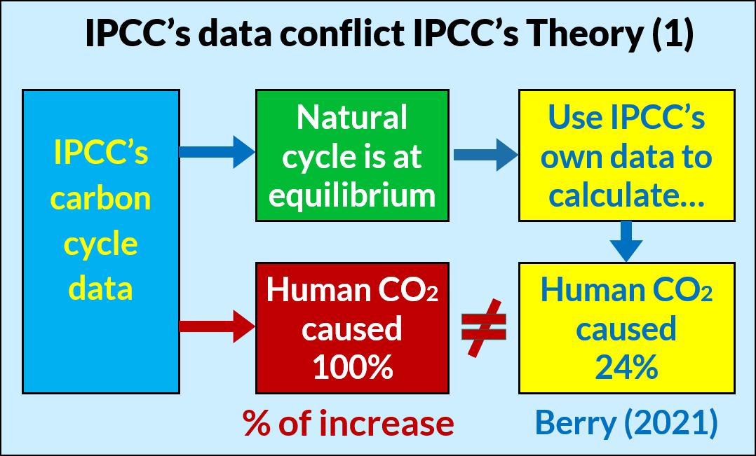
Fig. 6 shows IPCC’s two carbon cycles, natural and human.

IPCC’s true human carbon cycle predicts human CO2 caused 24% of the CO2 increase by 2020 and nature caused 76%.

However, IPCC’s Theory (1) human carbon cycle predicts human CO2 caused 100% of the CO2 increase. Therefore, Theory (1) is false because it conflicts with IPCC’s own data.

IPCC’s true human carbon cycle predicts human CO2 caused 24% of the CO2 increase by 2020 and nature caused 76%.

However, IPCC’s Theory (1) human carbon cycle predicts human CO2 caused 100% of the CO2 increase. Therefore, Theory (1) is false because it conflicts with IPCC’s own data.

Figure 5. IPCC’s natural and human carbon cycles according to IPCC’s Figure 6.1. The percentages show the distribution of carbon in the carbon cycle at equilibrium.

carbon cycle data to properly

3.7 Human carbon was too small before 1950

Fig. 7 shows data from 1820 to 2020. IPCC’s true human carbon cycle shows human carbon in the atmosphere as of 2020 was about 70 PgC. The measured carbon level was 290 PgC. Therefore, natural carbon added 220 PgC to the atmosphere.

Figure 7. The blue line shows the human CO2 level of IPCC’s true human carbon cycle. The black line is the measured carbon level. The red dotted line is the accumulated human total carbon inflow since 1750 assuming all human emissions remained in the atmosphere. The green dotted line is the accumulated natural inflows.

Figure 6. IPCC’s natural carbon cycle derives from data. IPCC’s Theory (1) human carbon cycle is not derived from data. Berry (2021) used IPCC’s natural

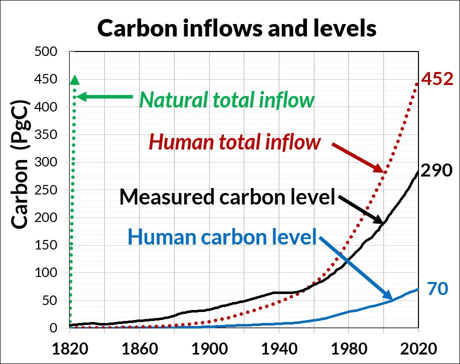
The accumulated human total inflow reaches 452 in 2020, much greater than the measured total in 2020. IPCC’s Theory (1) believers use this difference to claim Theory (1) is true. However, their claim is invalid because they do not subtract outflow.

Before 1950, human total inflow was less than the measured carbon level. So, human carbon emissions were insufficient to have produced the measured carbon level. This alone falsifies IPCC’s Theory (1).

Finally, the green dotted line shows the accumulated natural inflow. Yet, no one argues this proves natural carbon caused all the added carbon. This illustrates how arguments that use accumulated inflows do not prove a cause of the increase.

4. Theory (1) argument uses circular reasoning

4.1 Theory (1) believers reject separate carbon-cycles

The IPCC defines two separate carbon cycles, human and natural. Berry (2021) shows why it is better to calculate human and natural carbon cycles independently rather than using their total because two cycles provide more, independent information.

However, Andrews (2023) argues for the true believers,

In their quest to determine the fraction of anthropogenic carbon in the present atmosphere Harde and Salby, Berry, and Schroder focus on anthropogenic and natural carbon separately. This complicates their analysis, and they miss the simple conclusions made here.

What they do find is natural carbon is accumulating in the atmosphere faster than human carbon, and indeed it is! Nothing in the analysis presented here conflicts with this fact.

Anthropogenic carbon can be the cause of the entire Industrial Age increase without being a large part of the present atmospheric composition.

Of course, it is the total atmospheric carbon that impacts climate, and the above analysis leaves no doubt where the increase in the total is coming from.

Tracking anthropogenic carbon separately from natural carbon is a distraction, which is why few papers in the serious peer-reviewed literature do so.

Andrews‘ every paragraph above is wrong. His arguments fail physics and contradict IPCC’s separation of human and natural carbon cycles.

Good physicists use all the information available to solve problems. Andrews discards important data and consequently makes an invalid circular argument.

4.2 Theory (1) believers use circular reasoning

Berry (2021) wrote,

Another invalid argument used to support the IPCC basic assumption is, because nature absorbs human carbon from the atmosphere, therefore nature cannot add carbon to the atmosphere. This argument neglects the physics model superposition principle that explains why the natural carbon cycle is independent of the human carbon cycle.

Andrews argues incorrectly for Theory (1) believers [brackets show Berry’s replies],

1. Because the carbon from human emissions during this period exceeds the rise in atmospheric total carbon, we know immediately that land and sea reservoirs together have been net sinks, not sources, of total carbon during this period. [No, we do not. This is circular reasoning.]

2. We can be sure of this without knowledge of the detailed inventory changes of individual non-atmospheric reservoirs. [No, we cannot.]

3. This is not a model dependent result. It is a simple statement based on carbon conservation,

data on emissions and atmospheric levels, and arithmetic. [No, it is based on circular reasoning.]

4. Note that this conclusion contains no assumption whatsoever about the constancy of natural carbon in this period. [No, it inherently assumes Theory (1) is true.]

5. In fact, the primary conclusion of Ballantyne is that non-atmospheric natural reservoirs –during the 50-year period studied – have not only increased their carbon inventory, they have also increased the rate at which they are doing so in response to the higher atmospheric levels. [No. Ballantyne and “in response to the higher atmospheric levels” assume Theory (1) is true.]

6. Nor does the conclusion rely on treating “human” and “natural” carbon differently as (Harde and Salby 2021) and (Berry 2021) both allege. [No, because Theory (1) requires different e-times for natural and human CO2.]

7. Net Global Uptake is simply what is left over after atmospheric accumulation has been subtracted from total emissions. If more carbon was injected into the atmosphere by human activities than stayed there, it had to have gone somewhere else. [No, this claim is based on circular reasoning.]

Let’s take this one little baby step at a time because too many potentially smart PhDs are fooled by the argument repeated by Andrews. (If this does not work, we may publish a coloring book.)

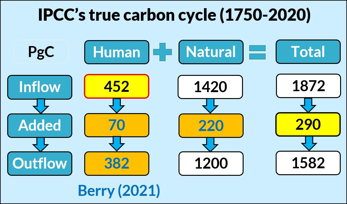
Fig. 8 shows a simple spreadsheet. The rows are Inflow, Added, and Outflow totaled from 1750 to 2020. The columns are the Human, Natural, and Total.

For terminology, we use our terms relevant to the atmosphere to replace Andrews’ terms as follows:

1. Human Inflow = Cumulative Human Emissions = 452 PgC

2. Human + Natural Added = Atmospheric Accumulation = 290 PgC

3. Total Inflow – Total Added = Net Global Uptake = 162 PgC

4. Total Outflow = Net Global Uptake = 162 PgC

Net Global Uptake is simply Total Outflow. So, why use it? The proper way to view the effects of human and natural carbon inflow is shown in Figs. 8 and 9.

The difference between Berry’s numbers and Andrews numbers is not relevant because Andrews totals the data from 1960 to 2010 while Berry totals the data from 1750 to 2020. These differences have no bearing on the logic of this discussion.

Fig. 8 shows the only values derived from data: Human Inflow = 452 PgC and Total Added = 290 PgC (from Fig. 7). These values tell us nothing about the Human Added vs the Natural Added. To make his argument, Andrews assumes Theory (1) is true (without realizing he made this assumption) and thereby puts zeros in the natural column, forcing Total Inflow to equal Human Inflow.

Then he subtracts the Total Added from his assumed Total Inflow to get 162 for Total Outflow, that he calls Net Global Uptake.

Andrews’ argument requires all natural components to be zero, which is the same as assuming Theory (1) is true. To assume the result to prove the result is called circular reasoning.

The only way to separate Human Added from Natural Added is to calculate IPCC’s true human carbon cycle. Berry (2021) does this using IPCC’s own data.

This makes the Natural Added equal to 220 PgC and Human Outflow equal to 382 PgC. The numbers in the white boxes are estimates that keep the human and natural flows proportional.

Fig. 9 contradicts the believers‘ invalid argument that because “nature” absorbs human carbon (Human Outflow), nature can’t also add carbon (Natural Added)

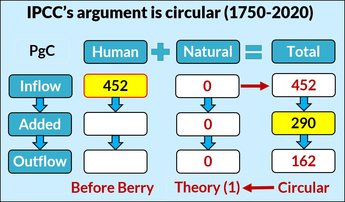
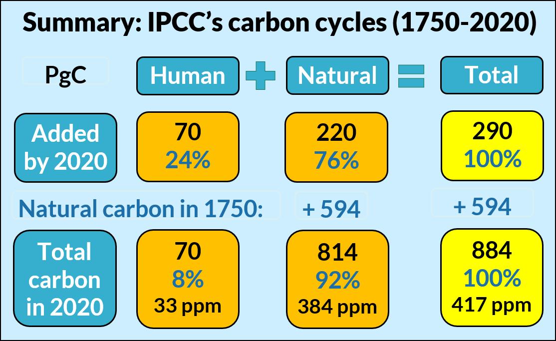
Fig. 10 shows the summary of IPCC’s true carbon cycle. As of 2020, human carbon was 24% of the Total Added, and 8% of the Total in the Atmosphere. These results prove IPCC’s Theory (1) is false and Andrews (2023) is science fiction.

Figure 8. Carbon sums from 1750 to 2020. Carbon cycle overview shows the Inflow, Added, and Outflow for the Human, Natural, and Total carbon cycles.

Fig. 9 updates Fig 8 by including Human Added of 70 PgC according to IPCC’s true human carbon cycle.

Figure 9. Carbon sums from 1750 to 2020. We insert 70 PgC for Human Added according to IPCC’s true human carbon cycle. This Natural Added is 220 PgC and Human Outflow is 382 PgC.

Andrews boldly claims,

As the disconnect between current inventories and fundamental causes is subtle, an analogy may be helpful for understanding it. Cawley (2011) proposed a good one, worth repeating verbatim here:

Consider a married couple, who keep their joint savings in a large jar. The husband, who works in Belgium, deposits six euros a week, always in the form of six one-euro coins minted in Belgium but makes no withdrawals.

His wife, who works in France, deposits 190 euros a week, always in the form of 190 oneeuro coins, all minted in France. Unlike her husband, however, she also takes out 193 euro per week, drawn at random from the coins in the jar.

At the outset of their marriage, the couple’s savings consisted of the 597 French-minted oneeuro coins comprising her savings.

Clearly, if this situation continued for some time, the couple’s savings would steadily rise by 3 euros per week (the net difference between total deposits and withdrawals).

It is equally obvious that the increase in their savings was due solely to the relatively small contributions made by the husband, as the wife consistently spent a little more each week than she saved.

Andrews adds for emphasis, showing he misunderstands the physics:

Cawley goes to the trouble of showing with a Monte Carlo simulation that, after some time, Belgian coins make up only 3% of the inventory, even though they accounted completely for the savings increase.

In a like manner human carbon, while a relatively small percentage of carbon in the present atmosphere, is completely responsible for the increase.

If Andrews had read and understood Berry’s physics model, he might have understood that Cawley’s analogy proves Berry’s physics model is valid. Here is why.

Figure 10. Human carbon is 24% of Total Added and 8% of Total in Atmosphere.

4.3 Cawley’s analogy confirms Berry’s model

Edwin X Berry: Nature controls the CO2 increase

Let S = Savings = 597 F

Let B = Belgium Deposits = 6 B per week

Let F = France Deposits = 190 F per week

Let W = Withdrawals = 193 (B or F) per week,

Use physics model (3) with Te = 1 to describe the weekly evolution of B and F in the money jar,

The final terms in (11) represent the probability of selecting either a B or F coin.

In this analogy, the levels of B and F are increasing so there are no fixed balance levels. However, we can calculate the relative balance levels that depend upon their relative inflows.

Use physics model (4) to find their relative balance levels,

Equation (12a) shows the final percent of B in the jar is 3.06 percent, which is Cawley’s result

The difference is we don’t need no stinkin’ Monte Carlo simulation to solve this problem. Berry’s physics model gives the answer at once. That is the power of the physics model.

Andrews is fooled by Cawley‘s analogy.

Andrews incorrectly claims for Theory (1) believers:

We have seen that the statement “Human carbon in the present atmosphere is only 30% of the Industrial Age increase” is not the same as “Human emissions caused only 30% of the increase.”

Anthropogenic carbon can be the cause of the entire Industrial Age increase without being a large part of the present atmospheric composition.

Andrews thinks the B coins represent human carbon emissions, and argues they “accounted completely for the savings increase.”

However, the B coins do not account for all the increase, just as human carbon emissions do not account for all the CO2 increase. The B coins account for only 3.06% of the increase and the F coins account for 96.94% of the increase. The B coins are also responsible for 3.06% of the money in the bank.

It does not matter how many B or F coins were in the jar in the beginning, or who withdraws the coins. The only thing that matters is the ratio (or percentage) of their balance levels which is the ratio (or percentage) of their inflows.

Cawley’s analogy proves Berry’s (2021) physics model is correct and powerful. Similarly, the best way to understand the impact of human and natural CO2 on the CO2 increase is to calculate IPCC’s true human carbon cycle independently as Berry (2021) has done.

Human and natural carbon cycles are independent. Therefore, a calculation that human carbon has produced 25% of the CO2 increase means it has caused 25% of the CO2 increase.

Andrews (2023) says incorrectly,

Ocean acidification has been observed and confirms what Net Global Uptake tells us: the primary reservoir, the oceans, have on balance globally been taking in net carbon, even while outgassing net carbon at some locations.

There are no data that show the net the source of the carbon added to the surface ocean. The data show levels, not flow directions. IPCC reports assume Theory (1) is true to then claim the added carbon comes from the atmosphere.

Berry (2021) shows it is more logical to assume that nature increased the natural carbon in the oceans, and this added ocean carbon flows into the atmosphere.

5. Why IPCC’s Theory (1) is false

5.1 IPCC’s Theory (1) needs a magic demon

IPCC (2007, p. 948) says the turnover time (T) for natural CO2 is about four years.

Carbon dioxide (CO2) is an extreme example. Its turnover time is only about four years because of the rapid exchange between the atmosphere and the ocean and terrestrial biota. However, IPCC (2013, p. 469) assumes human CO2 turnover time is much larger than four years, The removal of human-emitted CO2 from the atmosphere by natural processes will take a few hundred thousand years (high confidence).

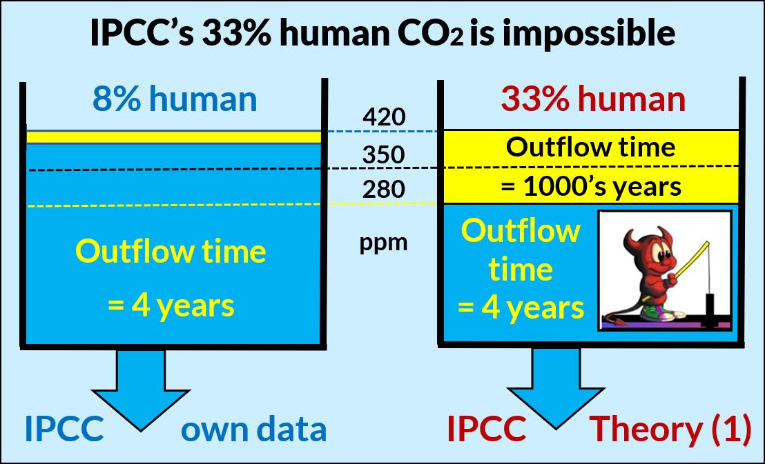
Fig. 11 compares the two scenarios: IPCC’s true human carbon cycle vs IPCC’s Theory (1).

• IPCC’s true human carbon cycle shows human carbon is 8% of atmospheric carbon as of 2020.

• IPCC’s Theory (1) claims human carbon is 33% of atmospheric carbon.

There are no data that show human CO2 stays in the atmosphere for thousands of years. IPCC makes this claim because Theory (1) requires this claim.

Levels (like 33%) must be supported by relative inflows. So, the Theory (1) claim that human carbon is 33% of atmospheric carbon requires the inflow of human carbon to be 33% of the total (human plus natural) inflow. IPCC’s own data show the inflow of human carbon is about 5% of the total carbon inflow.

To the first order approximation, the relative levels of human to natural CO2 follow the relative inflows of human to natural CO2, which produces their relative balance levels. (The second order

Figure 11. IPCC’s true human carbon cycle that says human carbon is 8% of the carbon increase. IPCC’s Theory (1) that says human carbon is 33% of the carbon increase.

Edwin X Berry: Nature controls the CO2 increase

approximation includes the human addition of new carbon to the carbon cycle.)

Therefore, to support its Theory (1), the IPCC contradicts physics to claim the human CO2 e-time is much larger than the natural CO2 e-time Andrews and others believe this charade.

So, IPCC’s Theory (1) requires a magic demon in the atmosphere to capture human CO2 and put it in a box with an e-time of 1000’s of years, while it lets natural CO2 flow freely out of the atmosphere with an e-time of 4 years.

But because human and natural CO2 molecules are identical, human and natural CO2 must have equal e-times, according to the physics Equivalence Principle. Therefore, Theory (1) is false.

5.2 δ14C data show human emissions are insignificant

We learned in Section 3.2 that inflows set balance levels, and levels always approaches their balance levels

The balance level of a mixture, like δ14C, is the non-dimensional ratio of the balance levels of its components. We used ratios of balance levels to quickly and accurately solve Cawley’s analogy. Forget Andrews‘ elaboration on isofluxes. Mixtures do not flow. Their components flow and their mixtures follow. The easiest way to understand components is with their relative balance levels, as we showed with Cawley’s analogy.

Fig. 12 shows δ14C data from 1955 to 2015. Turnbull et al. (2017) processed δ14C data for Wellington, New Zealand, from 1954 to 2014.

The “natural” δ14C balance level, defined by the average measured level before 1950, is zero, as shown by the blue horizontal line.

Figure 12. δ14C data (Turnbull et al., 2017, black line) show it has returned toward its original balance level of zero even as the 12C level increased.

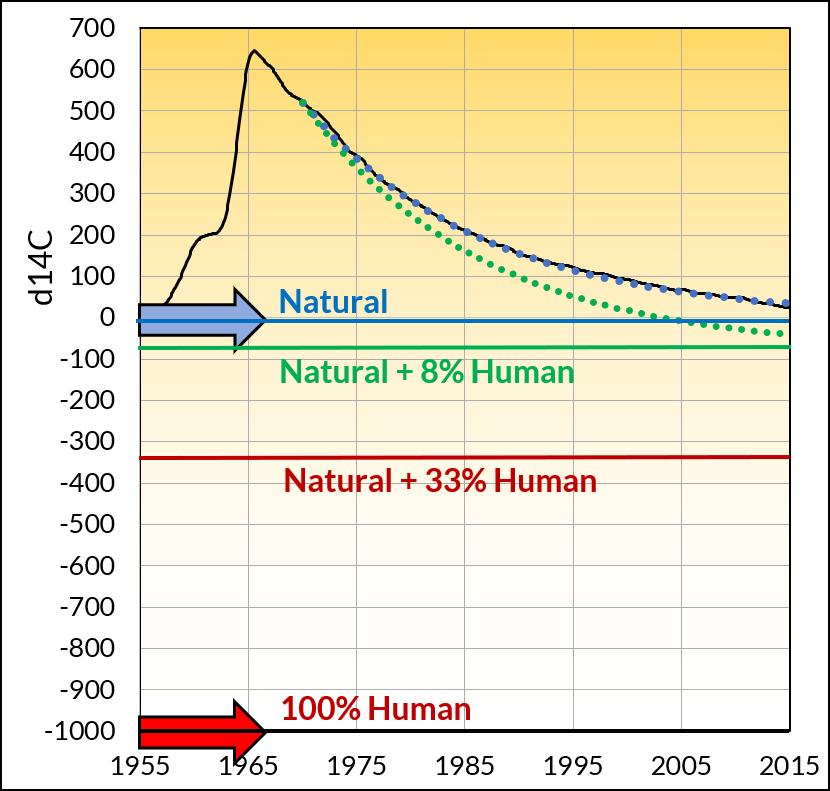
The blue dotted lines that fit the δ14C decrease are a mathematical fit of (8) with a balance level of zero and an e-time of 16.5 years. The close mathematical fit to the δ14C data shows the δ14C natural balance level remained near zero and its e-time has been constant, at least since 1970.

Since 1970, the δ14C level decreased toward its natural balance level of zero, showing the natural δ14C balance level has not changed.

So, while the atomic bomb tests in the 1960s added 14C to the atmosphere, thereby increasing δ14C, the bomb tests did not change the δ14C balance level of zero

Human carbon has no 14C, so its δ14C level is -1000, as shown in Fig. 12. Human carbon will dilute δ14C inflow and thereby lower the δ14C balance level below zero.

If human CO2 were truly 33% of atmospheric CO2 as IPCC’s Theory (1) claims, this would lower the δ14C balance level to -330 as shown by the horizontal red line. Data show this has not happened, so IPCC’s Theory (1) is false.

If human CO2 were 8% of atmospheric CO2 as Berry (2021) calculates using IPCC’s data, this would lower the δ14C balance level to -80 as shown by the horizontal green line. But even this has not happened. Fig. 12 indicates human carbon in the atmosphere is less than 4%, contradicting IPCC’s natural carbon cycle data.

The δ14C balance level has remained near zero, showing human 12C inflow has not lowered the δ14C balance level. Graven et al. (2020) agree. Their Figure 6 shows the observed δ14C is still above zero as of about 2015 and it is not headed toward a negative value.

The Graven et al. plot of δ14C below zero are not data but are projections after 2020 by an unreferenced model that is likely a climate model. We cannot trust climate models because they assume Theory (1) is true

The bottom line is δ14C data prove IPCC’s Theory (1) is false.

5.3 A new theory: nature keeps δ14C balance level constant

Our sections above have proved Theory (1) is false. In this section, we propose a new theory that is open to being proved false.

Berry’s calculation of IPCC’s true human carbon cycle is deductive and reproducible. By contrast, this δ14C argument is inductive and a theory subject to being proved wrong.

The first question is, what caused 14C to increase after 2000?

The second question is, what keeps the δ14C balance level near zero?

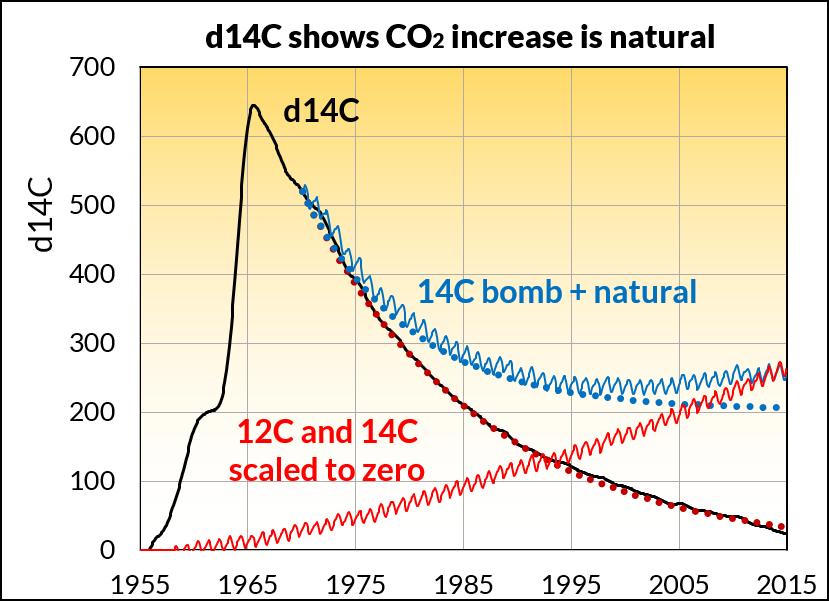
Fig. 13, (improved from Berry, 2021) plots the following data:

• δ14C (solid black line) and its curve fit after 1970 (dotted red line).

• 12C increase scaled to zero (red sawtooth line).

• 14C increase scaled to zero, is identical to the 12C increase.

• 14C total of natural plus bomb (blue sawtooth line).

As in Fig. 12, (8) fits the δ14C data from 1970 to 2014 with a constant e-time of 16.5 years and constant balance level of zero.

The blue dotted line is a curve fit to the 14C data using (8). This fit shows 14CO2 has an e-time of 10.0 years. Harde and Salby (2021) found the same value using a different method.

The 12C increases since 1955 (red sawtooth line) following Graven et al. (2020) and is scaled to fit zero in 1957 by multiplying ppm data by 3.1676.

δ14C is a function of the ratio of 14C/12C. The components, 14C and 12C, flow independently. Yet, δ14C has kept its balance level near zero for a long time.

Andrews (2023) asks,

If the ~30% increase [of 14C] does not include lingering bomb carbon as it certainly appears to, what caused it?

Andrews thinks Caldeira et al. (1998) have the correct answer. They say the flow of human carbon from the atmosphere into the oceans drives 14C out of the oceans and into the atmosphere. They predict that 14C will go up after 1990, but they also predict δ14C will go negative after 2010. However, the δ14C balance level has remained at zero which contradicts their predictions, and the Caldeira et al. model assumes Theory (1) is true, which negates their conclusions.

Harde and Salby (2021) present a better model. They assume the 14CO2 and 12CO2 balance levels have increased in proportion due to the re-emission of 12C and 14C from external reservoirs in proportion to their direct absorption rate, thereby keeping δ C14 close to zero.

We propose another theory for the increase in 14C, that extends Harde and Salby (2021). Our theory says that, somehow, through rain and shine, nature keeps δ14C near zero.

Our theory says, the rise in 12C, while keeping δ14C = 0, causes the 14C increase. This correctly predicts the observed increase in 14C.

Our theory is based on the following observations:

1. δ14C has remained near zero for the last, say, 100,000 years, sufficient to allow carbon dating. It is likely that the 12CO2 and 14CO2 levels have changed up and down during that time.

2. δ14C decreased smoothly since 1970 toward its original balance level of zero with a constant e-time of 16.5 years.

Figure 13. δ14C data (Turnbull et al., 2017, black line), the physics model fit to δ14C (red dotted line), 12C scaled to zero (red sawtooth line), and 14C (blue sawtooth line) total of natural plus bomb. The dotted blue line is a curve fit to the 14C data.

3. The δ14C balance level stayed near zero throughout the bomb pulse.

We cannot explain how nature may have kept the δ14C balance level and e-time constant. But we cannot accept that these have remained constant by mere coincidence. Somehow, nature must control the δ14C balance level that has remained unchanged since 1950

The 14C natural (non-bomb) increase since 1955 is the same line as the 12C increase because the δ14C balance level remained near zero.

Were it not for the bomb 14C, the natural increase in 14C (blue sawtooth line) would have followed the 12C increase (red sawtooth line) while δ14C remained at zero.

It may be easier to follow this if we imagine two separate carbon cycles, one for natural 14C and the other for bomb 14C. Then we see that the bomb 14C is depleted by 2015 and the continued 14C increase is caused by the natural 12C increase.

This is the simplest (Occam’s Razor) explanation for the increase in 14C. That does not mean it is correct, but it is a theory we can use until someone proves it is false.

5.4 Equilibrium percentage levels sets effect of human CO2

Pollard (2022) determined the global CO2 emissions from freshwater ecosystems is some 60 times larger than IPCC’s data show. (See Figure 4, Section 3.5.)

To find the significance of this adjustment to IPCC’s data for its natural carbon cycle at equilibrium, we inserted this change into the physics carbon cycle program of Berry (2021). Since IPCC’s equilibrium natural carbon cycle levels are unchanged, Pollard’s new data changes some flows and e-times reported in Berry (2021).

First, it changes the flows between the land and atmosphere reservoirs from 108 PgC per year to 166 PgC per year. Second, it changes the e-times T12 from 23.15 years to 12.96 years, and T21 from 5.45 years to 3.55 years, as needed to keep IPCC’s levels at equilibrium. The effect of these changes on the (Berry, 2021) predicted human-caused CO2 increase of 33 ppm as of 2020 is zero.

This result shows the equilibrium reservoir levels, rather than the flows between the reservoirs, determine the effect of human CO2 emissions on the increase in atmospheric CO2. Therefore, research can focus on getting more accurate measurements of the levels of the natural carbon cycle because changes in flows will be compensated by changes in e-times.

To test the model effect of changing the carbon reservoir levels, we doubled the IPCC equilibrium levels in Berry’s physics model to 4300 PgC for land, 1800 PgC for surface ocean, and 80,891 PgC for deep ocean. The atmosphere level stayed the same because it is set by good data.

To keep these new levels at equilibrium required setting the following e-times: T12 to 7.65 years, T21 to 1.05 years, and T23 to 4.90 years. The ocean e-times stayed the same, suggesting the carbon level in the land reservoir has the strongest effect on the human increase in the CO2 level. These changes reduced the CO2 increase caused by human emissions as of 2020 from 33 ppm to 18 ppm. So, to the first approximation, doubling the equilibrium levels for land, surface ocean, and deep ocean reduced the human CO2 effect by about one-half.

6. Conclusions

IPCC’s Theory (1) assumes incorrectly that human CO2 is the dominant cause of the CO2 increase above 280 ppm, or since 1750. Ardent Theory (1) believers include the American Meteorological Society, American Physical Society, CO2 Coalition, Heartland Institute, and most schools, universities, and science teachers in America and the world.

IPCC’s Theory (1) fails because it is based on invalid physics and circular reasoning. This proof

that Theory (1) is false undermines the whole scientific and political thesis of human-caused climate change.

Until Andrews (2023), Theory (1) believers censored and ignored proofs that Theory (1) is false. Andrews published their best arguments to support IPCC’s Theory (1).

Berry’s (2021) carbon cycle model supersedes other IPCC carbon cycle models in simplicity and accuracy. It uniquely replicates IPCC’s natural carbon cycle.

Berry (2021) used IPCC’s own natural carbon cycle data to calculate IPCC’s true human carbon cycle. This true human carbon cycle predicts human carbon emissions have added only 33 ppm to atmospheric CO2 as of 2020 while natural CO2 emissions added 100 ppm of the CO2 above 280 ppm, proving Theory (1) is false. This 33 ppm is 8% of the carbon in the atmosphere in 2020. In addition, δ14C data show natural CO2 emissions dominate human CO2 emissions, proving Theory (1) is false. The δ14C data further suggest IPCC’s natural carbon cycle data overpredict the effect of human CO2 on atmospheric CO2, and lower the 8% of human carbon in the atmosphere calculated from IPCC’s data to less than 4%.

Pollard’s (2022) determination that freshwater systems emit 60 times more CO2 than IPCC’s data show, led us to conclude the equilibrium level percentages of the natural carbon cycle control the effect of human CO2 emissions on the CO2 increase.

The relative equilibrium percentage levels of available natural carbon in land, air, surface ocean, and deep ocean is the strongest predictor of the effect of human carbon on atmospheric CO2 because the independent human carbon cycle seeks the same percentage levels as the natural carbon cycle at equilibrium. For example, if the carbon levels of land, surface ocean, and deep ocean were each doubled, the human-caused CO2 in the atmospheric would be reduced by about half, or to 18 ppm which would be 4% of the carbon in the atmosphere

The bomb-caused increase in 14C, and therefore in δ14C, is now almost depleted as δ14C has returned to its original balance level of zero. Yet the 14C level is now higher than in 1950. To explain this 14C increase, we propose a theory that says nature keeps the δ14C balance level equal to zero. This theory correctly predicts the non-bomb 14C increase since 1950 is caused by the 12C increase while nature kept the δ14C balance level equal to zero. This is the simplest (Occam’s Razor) explanation for the non-bomb 14C increase since 1950

Appendix: Andrews’ fundamental errors

We all make progress step by step. Berry (2019) made several advancements and Berry (2021) extended the knowledge in Berry (2019).

Andrews (2023) makes the following fundamental, disqualifying errors:

1. Assumes Theory (1) is true when that is the subject under discussion.

2. Uses circular reasoning to argue Theory (1) is true.

3. Omits the natural carbon cycle in his Figure 1 arguments.

4. Does not realize this omission caused his argument to be circular.

5. Does not treat human and natural carbon cycles independently

6. Does not realize Theory (1) uses different e-times for human and natural CO2

7. Uses isoflux arguments where he should have used balance levels.

8. Thinks Cawley’s analogy supports Adrews but Cawley’s analogy supports Berry (2021).

9. Uses the meaningless term “characteristic time” rather than e-time.

10. Says “characteristic time for the mixing can be seen to be about one decade” without referencing Berry (2021) and Harde and Salby (2021) who were the first to calculate,

Edwin X Berry: Nature controls the CO2 increase

independently, the 14CO2 e-time is 10.0 years.

11. Says, incorrectly, the increase of 14CO2 after 2000 was caused by the bomb 14CO2

12. Says, without proof, “Eventually, around 2000, 14C/Ctot in the atmosphere was again less than it was in the oceans for the first time since the early 1950’s. This again caused a net flow, an isoflux, of 14C from the oceans to the atmosphere.”

13. Says, incorrectly, “ quantitative analyses have been performed by (Caldiera et al.1998), and more recently by (Graven et al. 2020). The Caldeira analysis preceded and anticipated the rise in 14C concentration beginning about 2000.”

14. Says, incorrectly, “Isoflux effects explain and dominate the evolution of 14C distributions… over the last 100 years.”

15. His bad science includes (a) omitting data available to solve a problem, (b) not recognizing his invalid assumptions, (c) using circular reasoning, and (d) using complicated theories when simpler theories are available.

16. Says “That progress is helped when the originators of the wrong ideas acknowledge their errors and find constructive ways to contribute,” but he does not apply his suggestion to himself

17. Says “Successful predictions are the hallmark of good science,” incorrectly suggesting correct predictions prove a theory is true.

18. Says “Scientific progress also relies on the use of empirical data to weed out ideas that may be original but are also just plain wrong,” but he cannot prove Berry (2021) is wrong

19. Says “The unconventional ideas critiqued here have been around for well over a decade. It should not have been necessary for this article to refer to a 2011 paper to, once again, refute them,” when he has not proved Berry (2021) is wrong and Cawley (2011) proves Andrews is wrong and Berry is correct.

Guest-Editor: Jan-Erik Solheim; Reviewers: anonymous.

Acknowledgements

My thanks to all who have helped me continue my climate physics research by commenting and challenging me on my website, by reviewing my papers, by encouraging me to pusue excellence, by simply being my friend, and especially to my wife, Valerie, who has been essential to my continuing research work.

Funding

The author received no financial support for this work.

Conflicts of Interest

The Author declares he has no known competing financial interests or personal relationships that could have appeared to influence the work reported in this paper.

References

Andrews, D.E. 2023: Clear Thinking about Atmospheric CO2. Science of Climate Change, vol. 3.1, pp 1-13. https://doi.org/10.53234/scc202301/20

Berry, E.X, 1967: Cloud droplet growth by collection. J. Atmos. Sci. 24, 688-701. DOI:

Edwin X Berry: Nature controls the CO2 increase

https://doi.org/10.1175/1520-0469(1967)024<0688:CDGBC>2.0.CO;2

Berry, E.X, 1969: A mathematical framework for cloud models. J. Atmos. Sci. 26, 109-111. https://moam.info/a-mathematical-framework-for-cloud-modelsedberrycom_59a6a1c81723dd0c40321bda.html

Berry, E. X and Reinhardt, R.L. 1974a: An analysis of cloud drop growth by collection. Part I. Double distributions. J. Atmos. Sci., 31, 1814–1824. https://doi.org/10.1175/15200469(1974)031<1814:AAOCDG>2.0.CO;2

Berry, E. X and Reinhardt, R.L. 1974b: An analysis of cloud drop growth by collection. Part II. Single initial distributions. J. Atmos. Sci., 31, 1825–1831. https://doi.org/10.1175/15200469(1974)031<1825:AAOCDG>2.0.CO;2

Berry, E. X and Reinhardt, R.L. 1974c: An analysis of cloud drop growth by collection. Part III. Accretion and self-collection. J. Atmos. Sci., 31, 2118–2126. https://doi.org/10.1175/15200469(1974)031<2118:AAOCDG>2.0.CO;2

Berry, E. X and Reinhardt, R.L. 1974d: An analysis of cloud drop growth by collection. Part IV. A new parameterization. J. Atmos. Sci., 31, 2127–2135. https://doi.org/10.1175/15200469(1974)031<2127:AAOCDG>2.0.CO;2

Berry, E.X, 2019: Human CO2 emissions have little effect on atmospheric CO2 International Journal of Atmospheric and Oceanic Sciences. Volume 3, Issue 1, June, pp 13-26.

https://doi.org/10.11648/j.ijaos.20190301.13

Berry, E.X, 2020: Climate Miracle: There is no climate crisis. Nature controls the climate Published in the United States by Amazon. 70 pp. https://www.amazon.com/dp/B08LCD1YC3/ Berry, E.X, 2021: The Impact of Human CO2 on Atmospheric CO2, Science of Climate Change, vol. 1, no.2, pp 1-46. https://doi.org/10.53234/scc202112/13

Burton, D. and G. Wrightstone, 2022: The CO2 Coalition is wrong because its physics is wrong CO2 Coalition and Heartland censor good science. (edberry.com)

Caldeira, K., Raul,G. H., and Duffy,P. B.,1998: Predicted net efflux of radiocarbon from the ocean and increase in atmospheric radiocarbon content. Geophysical Research Letters, 25(20), 3811-3814. https://doi.org/10.1029/2001GL014234

Cawley, G. C., 2011: On the atmospheric residence time of anthropogenically sourced CO2.” Energy Fuels 25, 5503–5513, https://dx.doi.org/10.1021/ef200914u.

Forrester, J.W., 1968, 2022: Principles of Systems. System Dynamics Society. 392 pp. Principles of Systems: Text and Workbook Chapters 1 through 10: Forrester, Jay W: 9781935056188: Amazon.com: Books

Graven, H., Keeling, R.F., & Rogelj, J. ,2020: Changes to carbon isotopes in atmospheric CO2 over the industrial era and into the future Global Biochemical Cycles, 34, e2019GB006170. https://doi.org/10.1029/2019GB006170

Harde, H. 2017: Scrutinizing the carbon cycle and CO2 residence time in the atmosphere Global and Planetary Change. 152, 19-26. https://doi.org/10.1016/j.gloplacha.2017.02.009

Harde, H. 2019: What Humans Contribute to Atmospheric CO2: Comparison of Carbon Cycle Models with Observations. International Journal of Earth Sciences. Vol. 8, No. 3, pp. 139-159.

http://www.sciencepublishinggroup.com/journal/paperinfo?journalid=161& https://doi.org/10.11648/j.earth.20190803.13

Harde, H. and Salby, M. L. 2021: What Controls the Atmosphere CO2 Level? Science of Climate Change, Vol. 1, No. 1, August 2021, pp. 54-69. https://doi.org/10.53234/scc202111/28.

IPCC. 2007: Climate Change 2007 - The Physical Science Basis. Contribution of Working Group 1 to the Fourth Assessment Report of the IPCC. Annex 1: Glossary: Lifetime.

Edwin X Berry: Nature controls the CO2 increase

https://www.ipcc.ch/site/assets/uploads/2018/02/ar4-wg1-annexes-1.pdf

IPCC, 2013: Ciais, P., Sabine, C., Bala, G., Bopp, L., Brovkin, V., Canadell, J., Chhabra, A., DeFries, R., Galloway, J., Heimann, M., Jones, C., Le Quéré, C., Myneni, R.B., Piao, S., and Thornton, P. 2013: Carbon and Other Biogeochemical Cycles. In: Climate Change 2013: The Physical Science Basis. Contribution of Working Group I to the Fifth Assessment Report of the Intergovernmental Panel on Climate Change [Stocker, T.F., Qin, D., Plattner, G.-K., Tignor, M., Allen, S.K. Boschung, J., Nauels, A., Xia, Y., Bex, V., and Midgley, P.M. (eds.)]. Cambridge University Press, Cambridge, United Kingdom and New York, NY, USA.

https://www.ipcc.ch/site/assets/uploads/2018/02/WG1AR5_Chapter06_FINAL.pdf

Kemeny, J.G., J.L. Snell, 1960: Finite Markov Chains. Springer. 238 pp. Amazon.com: Finite Markov Chains: With a New Appendix "Generalization of a Fundamental Matrix" (Undergraduate Texts in Mathematics): 9780387901923: Kemeny, John G., Snell, J. Laurie: Books

Pickering, K., 2016: Comment on cause of CO2 increase Murry Salby: Atmospheric Carbon, 18 July 2016 (edberry.com)

Pollard, P.C., 2022: Globally, Freshwater Ecosystems Emit More CO2 Than the Burning of Fossil Fuels. Environ. Sci., 06 June 2022. https://doi.org/10.3389/fenvs.2022.904955

Salby, M.L. and Harde, H. 2021: Control of Atmospheric CO2: Part I: Relation of Carbon 14 to the Removal of CO2. Science of Climate Change, 1, no.2.

https://doi.org/10.53234/scc202112/210

Salby, M.L. and Harde, H. 2022: Theory of Increasing Greenhouse Gases Science of Climate Change, Vol. 2.3, pp 212-238. https://doi.org/10.53234/scc202212/17

Scarborough, J.B. 1966: Numerical Mathematical Analysis. Sixth Edition. The John Hopkins Press. 608 pp. Numerical Mathematical Analysis: Scarborough, Dr. William, Scarborough, James B.: 9780801805752: Amazon.com: Books

Segalstad, T.V. 1998: Carbon cycle modelling and the residence time of natural and anthropogenic atmospheric CO2: on the construction of the Greenhouse Effect Global Warming dogma. In: Bate, R. (Ed.): Global warming: the continuing debate. ESEF, Cambridge, U.K. (ISBN 0952773422): 184-219. http://www.CO2web.info/ESEF3VO2.pdf

Schroder, H., 2022: Less than half of the increase in atmospheric CO2 is due to the burning of fossil fuels Science of Climate Change vol. 2, no. 3, pp 1-19.

https://doi.org/10.53234/scc202112/17

Skrable, K., Chabot, G., French, C., 2022a: World Atmospheric CO2, Its 14C Specific Activity, Non-fossil Component, Anthropogenic Fossil Component, and Emissions (1750-2018), Health Physics: February 2022 - Volume 122 - Issue 2 - p 291-305 doi: 10.1097/HP.0000000000001485

Skrable, K., Chabot, G., French, C., 2022b: Components of CO2 in 1750 through 2018 Corrected for the Perturbation of the 14CO2 Bomb Spike”, Health Physics: November 2022Volume 123 - Issue 5 - p 392 https://doi.org/10.1097/HP.0000000000001606.

Turnbull, J.C., Mikaloff Fletcher, S.E., Ansell, I., Brailsford, G.W., Moss, R.C., Norris, M.W., and Steinkamp, K. 2017: Sixty years of radiocarbon dioxide measurements at Wellington, New Zealand: 1954–2014. Atmos. Chem. Phys., 17, pp. 14771–14784. https://doi.org/10.5194/acp17-14771-2017