Global warming false alarm: the bad science behind the United Nations assertion about man-made CO2

GLOBAL WARMING FALSE ALARM

THE BAD SCIENCE BEHIND THE UNITED NATIONS’ ASSERTION THAT MAN-MADE CO2 CAUSES GLOBAL WARMING

GLOBAL WARMING FALSE ALARM

THE BAD SCIENCE BEHIND THE UNITED NATIONS’ ASSERTION THAT MAN-MADE CO2 CAUSES GLOBAL WARMING

RALPH B. ALEXANDER

CANTERBURY PUBLISHING

Copyright © 2012 by Canterbury Publishing

Second edition, updated and revised, 2012

All rights reserved. No part of this publication may be reproduced, stored in a retrieval system, or transmitted, in any form or by any means, electronic, mechanical, photocopying, recording, or otherwise, without the prior written permission of the publisher, except for review purposes.

Published by Canterbury Publishing

P.O. Box 1731, Royal Oak Michigan 48068-1731

SAN 858-4133

Library of Congress Cataloging-in-Publication Data

Alexander, Ralph B.

Global warming false alarm: the bad science behind the United Nations’ assertion that man-made CO2 causes global warming / Ralph B. Alexander. p. cm.

Includes bibliographical references and index.

ISBN-13: 978-0-9840989-1-0 (pbk. : alk. paper)

ISBN-10: 0-9840989-1-7 (pbk. : alk. paper)

1. Global warming—Political aspects. 2. Climatic changes—Environmental aspects. 3. Carbon dioxide. I. Title.

QC981.8.G56A34 2009

2009905563

Book design by Karl Rouwhorst

Printed in the United States of America

he paper used in this publication meets the minimum requirements of the Permanence of Paper standard ANSI/NISO Z39.48-1992 (R2002).

-

-

Chapter 3: Computer Snake Oil ............. 53

It’s Only A Model Fitting An Elephant Clouding he Picture

Failed Predictions

- he Missing Atmospheric Hot Spot

- he Arctic And Antarctic

- Northern Vs Southern Hemisphere

- he Oceans

Chapter 4: CO2 Sense And Sensitivity ........

CO2 Feedback: False Positive?

- Negative Feedback In Satellite Data

CO2 Oversensitivity

Two-Faced CO2

67

Chapter 5: Doing What Comes Naturally..... 81

Nature’s Warming: he Sun

- Rhythms Of he Solar System

- Ampliication Mechanisms: Cosmic Rays From Outer Space

- Ampliication Mechanisms: Ozone

- Other Planets

- More IPCC Shenanigans: Solar Warming Minimized

Nature’s Warming: he Oceans

he Sun-Ocean Connection

he Paciic Decadal Oscillation (PDO)

Preface

Much has happened in the global warming arena since this book was irst published three years ago. Shortly ater the book came out, the Climategate scandal burst into the open and sent shock waves around the world. his was quickly followed by the ending in disarray of the overhyped Copenhagen climate summit, which failed to reach agreement on extending the UN Kyoto Protocol that attempts to limit greenhouse gas emissions.

Sincethen,amyriadofmistakesandnewexaggerationsbytheIPCCandclimate change alarmists have come to light, hysteria over weather extremes supposedly caused by man-made CO2 has reached new heights, an important experiment on cloud physics has been conducted, and the cooling trend that began in 2001 has shown no signs of letting up.

All these developments and more are covered in this revised edition, which contains approximately 50% new or updated material, including an expanded chapter on alternative explanations to CO2 as the main source of global warming. he only area where I’ve cut back is CO2 data, since there is little dispute over how much the level of CO2 in the atmosphere is rising.

he biggest change is to the endnotes. here are now more than 400 explanatory notes and scientiic references, the majority of references including URLs (Internet addresses) where the paper or article – either the complete document or a summary – can be accessed free of charge. However, URLs are not supplied for references within IPCC reports, which can be accessed online only by the chapter. he few other references that don’t include a URL can generally be accessed for a fee, but the fee is oten more than the cost of this book!

And, while the less technically inclined may not want to look up every reference, I highly recommend consulting at least the explanatory notes, as these oten contain important detail.

I’d like to thank Kevin Walter, who pushed me into embarking on a 2nd edition and gathered most of the background material for the chapter on alternatives (Chapter 5); Roger Cohen, for his constructive comments on the 1st edition and several other insights; Gordon Fulks, for drawing my attention to several current papers in climate science, through his Global Warming Realists email group; and my wife Claudia, for her continued support and tolerance of the incursions my writing has made into our leisure time.

August, 2012

Preface to 1st Edition

I wrote this book because I’m a scientist. Because I’m ofended that science is being perverted in the name of global warming – today’s environmental cause célèbre. Because the world seems to have lost its collective mind and substituted political belief for the spirit of scientiic inquiry.

Science is not a political belief system. Yes, scientists are human and have their biases, but the keystone of science is rational investigation. here’s nothing very rational nor investigative about much of the conventional wisdom on global warming, which is characterized more by a near religious zeal than by thoughtful evaluation of the evidence.

It’s the abuse of science by global warming alarmists that turned me into a skeptic about CO2. Until fairly recently, I was a fence sitter and willing to accept the possibility that recent climate change is the result of human activity, though I also had my doubts.

What irst changed my view was a college course on physical science that I taught a few years ago and that included a segment on global warming. Despite the fact that the course focused on the scientiic method, and on not accepting hypotheses without adequate testing or evidence, the textbook simply presented the alarmist line on man-made global warming without question.

To me, that made a mockery of the history of science presented in the course, which featured several examples of how mainstream scientiic thinking has sometimes been wrong in the past. At the very least, I felt that the other side of the global warming debate should have been discussed as well.

he experience induced me to take a second look at global warming. As I delved more deeply into the background material, I found myself steadily moving over to the skeptical camp and becoming more and more annoyed at the strident tone of most alarmist declarations – especially the assertion that “the debate is over”. Such an assertion would have appalled the famous 19th-century British biologist homas Huxley, oten regarded as one of the founding fathers of modern scientiic thought, who once said: “Skepticism is the highest of duties; blind faith the one unpardonable sin”.

his book takes the skeptics’ viewpoint on global warming, but with emphasis on the underlying science rather than the politics. My intention is as much to resurrect the tarnished reputation of scientiic endeavor as it is to convince you that CO2 has little to do with global warming.

Why have I taken it on myself to defend the honor of science?

It’s because I feel so strongly about my chosen profession. I’ve been interested in science since my childhood, when science was held in particularly high regard following the development in only a few years of nuclear power, the transistor (the basis of today’s computer chip), and rockets capable of sending man to the moon – along with advances in the biological sciences such as iguring out the structure of DNA.

Some of the gloss of those heady times later wore of, and there was an understandable backlash when it was realized that science didn’t have all the answers to our problems. Unfortunately, this reaction helped fuel the rise of “junk science”, based on ignorance and fear instead of the traditional scientiic method. And all that coincided with the start of the global warming debate about 20 years ago, so perhaps we shouldn’t be surprised that the debate has generated more heat than light.

Much of the book is critical of the UN’s Intergovernmental Panel on Climate Change (IPCC). hat’s because the current belief that global warming is caused by man-made CO2 stems largely from the IPCC’s climate assessment reports, as interpreted by the mass media and swallowed by the public at large.

More than anything else, it is the IPCC reports that have convinced me alarmists are wrong about CO2.

I’m not saying that the lengthy, detailed reports are full of bad science. hey do contain accurate and useful information in places, supplied by well-meaning climate researchers who are genuinely trying to piece together a coherent picture of the Earth’s climate system. But these scientists appear to be in the minority within the IPCC, which is dominated by other scientists and bureaucrats who manipulate the data and the reports for their own ends.

All of this is a sad commentary on the state of science today. It has taken more than two millennia to develop and reine the modern scientiic method to the point where we’ve been able to make major technological advances in a relatively short time. But if we continue to debase science as the IPCC and other political bodies do, our wonderful scientiic heritage will be lost.

he book is written for both the layman and the scientist, at a level that anyone with a high-school education including some basic science should be able to understand. However, even those who can’t comprehend the science in detail should be able to follow the general line of argument.

To convey the essence of global warming science in a readable and informative manner, I’ve kept technical material and scientiic jargon to a minimum in the main text. Scientists, and those nonscientists seeking more detail, will have to dig a little further by consulting the many endnotes (and the appendices) at the back of the book.

here are several people I want to thank. hese include my brother Patrick, who irst got me seriously interested in global warming and encouraged me to write this book; my colleagues Keith and Hillary Legg, for many discussions on the subject and useful suggestions; Jim Peden, who convinced me to actually start writing; Howard Hayden and Roy Spencer, for answering my questions; and my wife Claudia, for her unwavering support and encouragement as I took on what is still an unpopular cause.

May, 2009

Chapter 1: Climate Change Delusions

Science is under attack like never before, especially by global warming alarmists. he alarmists would have us believe that doomsday is near, that a catastrophe awaits the Earth unless we stop pumping carbon dioxide (CO2) into the atmosphere by burning fossil fuels. It’s CO2 that is causing the climate to change, insist the believers. If we don’t do something about this pesky gas right now, our planet and our way of life will be destroyed.

his is utter nonsense. Global warming may be real, but there’s hardly a shred of good scientiic evidence that it has very much to do with the amount of CO2 we’re producing, or even that temperatures have risen as much as warmists say.

Today’s climate change hysteria began 25 years ago with United Nations discussions that created the Intergovernmental Panel on Climate Change (IPCC). To climate change alarmists, the climate bible is a series of assessment reports issued by the IPCC about every six years. Based on the collective opinion of several hundred climate scientists, these reports are the source of the widely held belief, promulgated by Al Gore and other alarmists, that higher temperatures are the result of human activity.1

Unfortunately, nature has not been cooperating. Global temperatures have latlined or fallen since about 2001, throwing a monkey wrench into global warming theory that doesn’t allow for cooling because the CO2 level is constantly going upwards.

Not to be put out, the global warming faithful simply changed their tune. Global warming became climate change, despite the fact that the Earth’s climate had already been changing for thousands of years, long before industrializa-

tion boosted CO2. And the telltale sign that CO2 causes climate change became weather extremes instead of rising temperatures. Widespread wildires in Russia, severe looding in Pakistan, deadly tornadoes in the U.S., even harsh winters and record snowfalls – all of these are the result of man-made CO2, according to the alarmists.

How convenient. Just ignore the current cooling trend and blame every unusual weather event on CO2 and global warming. hat may help drive political action on climate change, but it’s not science. True science is based on rigorous logic and evidence, not blind faith in quasi-religious dogma.

he IPCC and global warmists spare no efort in telling us to stop climate change by curtailing or even ending emissions of CO2. Failure to act will mean even more extreme weather, colossal shits in rainfall patterns, and thawing of the polar ice caps. But if we care to look back at the 1930s or the 1950s, when the CO2 level was much lower than now, we’d see that terrible loods2 and droughts3 and melting ice caps4 are nothing new.

he alarmists have spun such a web of deception that any science contrary to the view of human-induced global warming is either ignored, played down, or deliberately distorted. News releases and scientiic papers that don’t adhere to the IPCC “party line” on CO2 are frequently sidelined by a barrage of attacks, sometimes vicious and personal.

Global warming skeptics have very diferent ideas about the origins of climate change. Unlike alarmists, skeptics believe that humans have little to do with global warming and dispute the notion that our CO2 emissions have any signiicant efect on climate. hey question the basic science behind the whole case for a human inluence on the climate system.

To skeptics, climate change is almost entirely a result of natural causes. herefore, there’s no point in passing legislation on CO2 emissions arising from the human presence on Earth – at least, no point in doing it to combat global warming.

Both groups defend their views vehemently, although the debate, if it can be called a debate, is mostly conducted out of public sight in the silent world of Internet blogs. Actual debates between the two sides are rare, alarmists repeatedly refusing invitations to publicly discuss the issues, usually on the grounds that their skeptic counterparts are “unqualiied” (read: dispute the conventional wisdom) or that there is nothing to discuss.

-2-

Until recently, the mainstream media presented the alarmist viewpoint almost exclusively, as if man-made global warming were an established fact, a belief that no longer needed to be questioned or debated. To my amazement, this standpoint has even been adopted by many of the world’s most eminent professional scientiic societies.

An important part of the belief in global warming orthodoxy is the deeply ingrained misconception that a scientiic consensus exists, that the scientiic community speaks with one voice on CO2 and climate change.

Because of this, skeptics have been frequently denigrated and even publicly viliied by alarmists. Even today, alarmists persist in bad-mouthing anyone who doesn’t subscribe to their convictions by calling them “deniers” – an attempt to link global warming skeptics with the immorality of Holocaust deniers 5

Dr. Rajendra Pachauri, who is the current IPCC chairman, has ridiculed those who question the so-called consensus by comparing skeptics to members of the Flat Earth Society, which he said6 probably has about a dozen members in modern times. Former U.S. Vice President Al Gore has made similar statements, claiming that “hey [Skeptics] are almost like the ones who still believe that the Moon landing was staged in a movie lot in Arizona.”7

he tide has turned, however, in the last few years and public opinion has now swung toward climate change skeptics. While the general public was evenly divided between alarmist and skeptical views of global warming when the 1st edition of this book was published three years ago, recent polls indicate that the percentage of skeptics in the public at large is currently around 60%.8, 9 National newspapers in several countries now carry regular articles that present skeptical opinions or question the notion that our climate is headed for disaster.

Among scientists, the percentage of skeptics is generally lower, perhaps only 10% to 20% for climate scientists. An opinion poll of several hundred climate scientists worldwide on the origins of global warming was carried out by Dennis Bray and Hans von Storch, irst in 1996 and again in 2003 and 2008. he 2008 survey, conducted online, found that approximately 14% of the climatologists polled believe that climate change in general is not due to human activity.10

A survey of 3,146 earth scientists the same year asked respondents if they thought human activity was contributing signiicantly to changing temperatures. Some 82% of those surveyed answered yes,11 suggesting that 18% of earth

scientists are global warming skeptics, although a speciic question about global warming or climate change was not asked.

It is clear from both polls nevertheless that a substantial number of climate scientists, even if not a majority, are global warming skeptics – over 370 of the earth scientists polled who regard themselves as climatologists (12% of 3,146),12 for example.

Subsequent studies have pegged the percentage of climate scientist skeptics as high as 16%13 and as low as 2-3%.14 However, the low estimate has been criticized on several grounds by climate scientists themselves, including some who are not global warming skeptics, such as Roger Pielke Jr. On the study minimizing the number of skeptics, Pielke Jr. commented that “… this paper simply reinforces the pathological politicization of climate science in policy debate.”15

Scientists overall are much more skeptical than climate scientists. In 2007, U.S. Senator James Inhofe held a Senate hearing on global warming and the media, in an efort to balance the media’s one-sided stance in presenting the science of climate change. he hearing’s oicial report16 included a list of about 400 scientists from over 20 countries who have voiced strong objections to the assumed consensus on human-caused global warming. he list of dissenting scientists is constantly updated, and had grown to more than 1,000 by December 2010.17

An ongoing project designed to attract skeptics on climate change is the “Petition Project” 18 Originally organized in 1998 by the Oregon Institute of Science and Medicine, in order to counter the then-widespread claim that further examination of global warming science was unnecessary, the Oregon petition has now been signed by more than 31,000 U.S. scientists.

However, the petition refers to “catastrophic heating” of the Earth’s atmosphere and “disruption” of the earth’s climate, rather than climate change as such. So, as in the survey of earth scientists that didn’t ask explicitly about global warming or climate change, the exact number of global warming skeptics among the Oregon petition signatories is uncertain. It’s clear though that the number is large.

But does it matter what other scientists or the general public think about global warming? Aren’t the vast majority of climate scientists right? hey’re the experts ater all, who, in their own words at least, “understand the nuances and scientiic basis of long-term climate processes”.11

If climatologists’ conclusions and prognostications for the future were based on solid experimental observations – the hallmark of genuine science – there would be good reason to believe them. But, as you’ll see shortly, the whole architecture of man-made global warming depends on unbridled faith in deicient computer models. And the poor science is compounded by the all-too-human need of climate scientists to preserve their jobs and research funding by reinforcing the prevailing wisdom on global warming.

Receipt of climate science funding has long depended on being able to airm that CO2 controls our climate. his connection has been used to intimidate global warming skeptics, as observed by well-known climate scientist Richard Lindzen, who is Alfred P. Sloan Professor of Atmospheric Science at MIT:

But there is a more sinister side to this feeding frenzy. Scientists who dissent from the alarmism have seen their grant funds disappear, their work derided, and themselves libeled as industry stooges, scientiic hacks or worse. Consequently, lies about climate change gain credence even when they ly in the face of the science that supposedly is their basis.19

As well as skeptical scientists who keep quiet out of fear, there are others who feel no particular need to make their views known in public. I was in that category myself before embarking on this book. What all this means is that any count of scientiic skeptics on global warming is bound to be an underestimate.

CORRUPTED SCIENCE

As a scientist, what I personally ind most troubling about the climate change debate is the gross misuse of science by those on the alarmist side. he worst public ofender is the IPCC, which long ago became the accepted authority for those convinced that global warming has human origins.

In this book, I will expose the most lagrant abuses of normal scientiic practice by the IPCC, and draw attention to the questionable assumptions and interpretations of data that the IPCC and its alarmist advocates have used to formulate their position on global warming.

his will involve looking at both the science – which we’ll do at a fairly basic level – and the methodology used to interpret the available climate data. Good science is based on what is called the scientiic method, a set of procedures estab-

lished over many centuries since the time of the ancient Greeks. In later chapters, we will see where the IPCC has not only gone wrong in its handling of climate data, but has also departed repeatedly from sound scientiic methodology – to the point of corruption in many instances.

But irst, let’s review what the IPCC is and what it has to say about global warming.

THE INTERGOVERNMENTAL PANEL ON CLIMATE CHANGE (IPCC)

he IPCC has always believed that global warming is man-made, ever since it was established in 1988. he organization was founded jointly by the UN Environment Programme and by the World Meteorological Organization (WMO), a group that works to standardize weather-related observations. he IPCC’s stated purpose was to assess “the scientiic, technical and socioeconomic information relevant for understanding the risk of human-induced climate change”.

But despite the implication in this statement that climate change caused by human activity was still in the future, it’s no secret that the UN and the IPCC believed it was already happening. hough cloaked in bureaucratic language, this presumption can be clearly seen in the terms of the mandate that included, in addition to wording on illing gaps in our climate knowledge, statements such as: Review of current and planned national/international policies related to the greenhouse gas issue; Scientiic and environmental assessments of all aspects of the greenhouse gas issue and the transfer of these assessments and other relevant information to governments and intergovernmental organisations to be taken into account in their policies ...20

In other words, the whole IPCC efort has always been biased toward the assertion that humans alone have caused the warming we now measure across the globe. his bias is a central part of all the panel’s publications and reports. By the IPCC’s own admission,21 even the irst report in 1990 “... made a persuasive, but not quantitative, case for anthropogenic [human-caused] interference with the climate system.”

Subsequent IPCC reports have reinforced the original conclusion, adding more and broader arguments for the existence of man-made warming, and putting

TABLE 1.1: PRINCIPAL IPCC ASSERTIoNS22 Assertion Conidence level

1. man-made Co2 and other greenhouse gases23 in the 100% atmosphere have increased markedly since 1750.

2. most of the global warming in the last 50 years At least 90% has been caused by these gases.

3. Temperatures in the Northern Hemisphere since At least 66% 1960 have been the highest of any 50-year period in the last 1,300 years.

4. Even greater warming will occur this century if we At least 90% continue to emit Co2 and other greenhouse gases.

WHAT’S WRONG WITH THIS PICTURE?

• Assertions 2, 3 and 4 are debatable (though assertion 1 is not in dispute) and may not be true at all.

• Conidence levels as high as 90% are totally unjustiied, because these three conclusions are based solely on computer models that are only crude approximations to the Earth’s climate.

Such high conidence levels have led to the false, unsupportable beliefs that there is “scientiic consensus” on human-induced climate change and that “the science is settled”.

The phrase “global warming gases” has become part of everyday usage, despite the lack of any proven connection between greenhouse gases and global warming.

numbers to this and other assertions (Table 1.1). Each successive report has sounded more and more conident that global warming is largely our own fault. By the time the Fourth Assessment Report was issued in 2007, the IPCC claimed to be up to 90% certain of its conviction that rising temperatures are caused by human activity

All of that would be unimportant were the IPCC not so powerful: numerous governments around the world, not to mention environmental groups and the general public, regard its word as climate gospel – to be taken as the absolute truth, without question. Its reports on global warming are far more widely read and quoted than most speeches by world leaders on any topic at all. he IPCC itself rightfully claims that its reports immediately become “standard works of reference”. his is an enviable position that most interest groups and professional societies can only dream of.

If the IPCC were simply an organization of climate scientists without any agenda other than to review and understand the many factors afecting the Earth’s climate, its pronouncements might be more believable. But the reality is that the IPCC is mostly made up of bureaucrats and government representatives, intent on validating the panel’s original assumption that global warming is a man-made phenomenon. Indeed, two of its three working groups and an associated task force all focus on the impact and mitigation of global warming, based on the underlying presumption that it is a direct result of human activities he other working group concentrates on the science, but shares the same biased assumption.

he IPCC’s climate scientists consist of working scientists who act as either authors (contributors) or reviewers of the organization’s reports. Writing and reviewing the 2007 report supposedly involved more than 3,750 people,24 of whom an estimated 2,000 were climate scientists according to press reports at the time. But of these, only a small percentage held a PhD degree – the most generally accepted measure of scientiic expertise.

In any case, both numbers have been shown to be overestimates, due to duplication of authors and reviewers.25 My best estimate is that less than a half, maybe only a third, of the 3,750 involved in producing the 2007 report were climate scientists.26

Many of those who were not climate scientists were not scientists at all: the academic participants listed by the IPCC include social scientists and geographers, and other contributors include civil engineers and even lawyers. his means that much of the scientiic analysis in IPCC reports comes from people who may not have the background to assess the science. No doubt that’s why there have been a number of accounts of IPCC climate scientists whose dissenting opinions have been suppressed or ignored. It’s not an approach that produces good science.

THE CO2 GLOBAL WARMING HYPOTHESIS

Carbon dioxide gets a bad rap these days. Although crops and trees need it in order to grow, and it’s the gas that gives sot drinks their izz, we humans are spewing vast quantities of CO2 into the air by burning coal and natural gas for energy and by driving cars. If you believe the global warming alarmists, all the CO2 we produce is what’s causing the mercury to rise around the world.

How could this be?

To answer that question, we need to examine the scientiic observations on which the CO2 theory is founded. Observations, or data gathering, are at the root of the scientiic method that I referred to earlier. But we’ll see that these data don’t necessarily mean climate change is a human phenomenon.

here are two observations that have sparked the debate on global warming, one involving temperatures and the other, CO2 levels:

1. Worldwide temperatures have been climbing on average since the middle of the 19th century, although they have recently fallen slightly, and

2. he amount of CO2 in the atmosphere has steadily increased over the same timespan, at an accelerating rate. Much of the extra CO2 comes from human activities, mainly the burning of coal, oil and natural gas.

If temperature and the CO2 concentration have both gone up (see Figure 1.1), then it’s reasonable to say they must be connected – right? Rising temperatures and higher atmospheric CO2 are indeed related, but this doesn’t necessarily explain global warming. he crucial question is how strongly are they related?

GLOBAL WARMING FALSE ALARM

We know that rising CO2 levels boost the Earth’s temperature, but this is only a minuscule efect, not enough to account for the warming that the world has seen. It’s entirely possible that higher temperatures are only weakly linked to the elevated CO2 level and that most of the temperature increase hasn’t come from CO2 at all, but from some other, natural source – many skeptics would say the sun or one of our oceans.

1.1: The Modern Temperature and CO2 Record

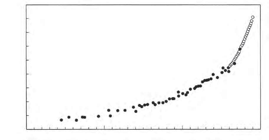
Sources: Temperature – Climatic Research Unit/Hadley Centre (HadCRU);27 CO2 (illed circles: Antarctic ice-core data, open circles: Mauna Loa Observatory measurements) – climateprediction.net.28

Figure

he climate change debate hinges on this issue, on how the separate observations about the Earth’s temperature and the CO2 content of its atmosphere should be interpreted.

According to the IPCC and global warming alarmists, the only possible interpretation is that the warming we have experienced is caused by the raised level of CO2. his conclusion is embodied in a scientiic hypothesis (Table 1.2), which explains the CO2–temperature connection in terms of what we call the greenhouse efect.

he greenhouse efect, named (though incorrectly) for the process that ripens tomatoes in a glass hothouse, is a well-understood scientiic phenomenon, originally explained by the French mathematician Joseph Fourier in the 1820s. Because it’s described at length elsewhere, I won’t go into detail here. A simpliied explanation is that greenhouse gases in the atmosphere act as a radiative blanket around the Earth, trapping some of the sun’s heat that would normally be radiated away.32 his makes the planet warmer than it would be without greenhouse gases.

A possible greenhouse connection between increased CO2 levels and higher temperatures was irst proposed by the Swedish chemist Svante Arrhenius, at the end of the 19th century. He later hypothesized that human activity could result in global warming.33 But it was not until the IPCC began publishing its climate reports in the 1990s that belief in the CO2 hypothesis became widespread.

Contrary to popular opinion, however, the major greenhouse gas in the atmosphere is not CO2, but water vapor (H2O). Water vapor accounts for about 70% of the Earth’s natural greenhouse efect and water droplets in clouds for another 20%, while CO2 contributes only a small percentage, between 4 and 8%, of the total. he other greenhouse gases are ozone, methane, nitrous oxide and chloroluorocarbons (CFCs, the gases formerly used in aerosol cans and refrigerators), which all make even smaller contributions to greenhouse warming.

Without the natural greenhouse efect – in the absence of any greenhouse gases at all – life on Earth as we know it would not exist. he globe would be cooler than it is now by about 33o Celsius (60o Fahrenheit), too chilly for most living organisms to survive.

hus, it’s deinitely possible in principle that adding to the store of existing greenhouse gases by putting more CO2 into the atmosphere could increase tem-

TABLE 1.2: THE Co2 HYPoTHESIS Observations

• Global surface temperatures have risen by approximately 0.8 o Celsius (1.4 o fahrenheit) since 1850.29

• The CO 2 level in the lower atmosphere has gone up as much as 37% in the same period,30 largely due to man-made Co2 emissions from factories and automobiles.

Hypothesis

Global warming is caused primarily by man-made Co2 in the atmosphere via the greenhouse effect, which says that greenhouse gases such as Co2 heat up the Earth.

WHAT’S WRONG WITH THIS HYPOTHESIS?31

1. The CO2 steady level problem: The Co2 level remained steady during previous global warming and cooling periods over the last 2,000 years – neither going up nor down as the average temperature rose and fell.

2. The CO2 ampliication problem: The climate change from extra Co2 is very small. A 37% upswing in Co2 causes only a tiny temperature increase, unless this increase is ampliied by water vapor in the atmosphere and by clouds. But we don’t know how big or small this ampliication is, or even if it’s an ampliication and not a diminution.

3. The CO2 lag problem: Historically, gains in atmospheric Co2 levels occurred several hundred years after the temperature went up. This Co2 lag, in the global warming period following an ice age, can’t be reconciled with today’s global warming, in which Co2 and temperature have risen together.

peratures. One place in the solar system where there is an abundance of CO2 and a pronounced greenhouse efect is the planet Venus.34 But the total amount of CO2 in the Earth’s atmosphere is still only very small: about 390 parts per million, or less than one twentieth of a percent. It takes an awful lot of CO2 to make an appreciable diference.

he critical issue is whether the extra CO2 that we’ve injected into the Earth’s atmosphere since industrialization began in the early 1800s is enough to bump up the temperature by the observed 0.8o Celsius (1.4o Fahrenheit).

It is on this question that climate change skeptics and alarmists difer most sharply. Skeptics say there’s no good evidence that man-made CO2 is playing any signiicant role in global warming. he alarmists, on the other hand, say everything points to the fact that it is.

COMPUTER MODEL FALLACIES

To skeptics, the IPCC’s claim that we can be more than 90% certain that global warming is entirely man-made borders on the absurd. As we’ll see, every single conclusion and prediction in all the IPCC reports is based on computer models of the Earth’s climate, and these theoretical models are far from the tools for accurate climate analysis and projection that the IPCC believes them to be.

I am not saying that computer models can’t play a useful role in simulating complex physical phenomena such as climate. It’s just that computer simulations are only as accurate as the underlying assumptions in the model.

If the assumptions in a particular computer model are based on established science, the predictions of the model are highly reliable – and a conidence level approaching 100% is warranted. A good example of this is the computer calculations used by the U.S. government to simulate explosions of nuclear weapons in its stockpile.

Back in the days when people worried about dangerous radioactive fallout from atmospheric testing of atomic bombs, worldwide political pressure led to the banning of atmospheric tests and the initiation of underground testing. But because some nuclear fallout occurs even when tests are carried out deep underground, computer simulations are now used as an alternative to conducting actual tests of the warheads. So accurate is the computer model in representing the science of nuclear explosions that the government believes it has an excellent

handle on the capabilities of its nuclear stockpile, and consequently feels no need to resume its previous real-world testing to conirm the strength of its nuclear deterrent.

hat’s the good news, for both nuclear weapons stewardship and the environment. But not all computer models are as sophisticated as those that mimic nuclear explosions, nor are the underlying physical processes as well understood or even known in many cases. Models that attempt to simulate the behavior of the universe, or of the human brain – both immensely complex systems, on different scales – are only in their infancy today and unable yet to make many useful predictions.

Climate models are in this category too. here’s a lot we’ve learned about the intricacies of the climate on our planet, but there’s also a great deal we don’t know. Our understanding of clouds and water vapor, of the interaction between the oceans and the atmosphere, and even the details of the sun’s efect on the Earth’s climate are all still at a primitive stage. hese factors can only be modeled crudely, and anything poorly understood is oten let out of the models altogether.

It makes no sense at all, therefore, to attach a conidence level of 90% (“very likely” in IPCC terminology) to the statement, for example, that greenhouse gases have caused most of the global warming that we see. A conidence level of a few percent might be closer to the mark. Even in the Bray and von Storch survey in 2008, only 50% of the climate scientists polled thought that the current theoretical understanding of climate change is adequate.35

THE SKEPTICS’ EXPLANATION: NATURAL CAUSES

Skeptics about the alarmist belief in human-induced climate change have an alternative explanation that doesn’t depend on bad science or demonization of critics to convey its message: the warming is predominantly natural, the result of one of nature’s many cycles. We already know there are cycles that have caused the Earth’s temperature to luctuate numerous times in the past.

What are these cycles?

One type of cycle that is deinitely not the cause of the current warming trend is regular but long-term changes in the Earth’s orbit around the sun. We learn in high school that the Earth goes around the sun in an elliptical path, and that it spins on an axis that is tilted. Over time, the elliptical orbit stretches and con-

tracts, the angle of tilt changes – on diferent timescales – and the Earth also wobbles on its axis, on yet another timescale.

he cumulative efect of all these slow dance moves by the Earth is that the amount of heat and light from the sun goes up and down over long periods of time, especially near the North Pole. his causes extended global warming and global cooling cycles, both of which can last for tens or even hundreds of thousands of years.

Prolonged cooling cycles are known as ice ages because of the massive ice sheets and glaciers that cover a lot of the planet. he next ice age is not expected for at least another 1,500 years, and maybe longer if current global warming persists.

But there are other natural cycles, many of which are shorter than the Earth’s orbital cycles, that could be inluencing our present climate – notably those associated with our sun. As we’ve seen, the sun’s heat energy, in combination with greenhouse gases (mostly water vapor) in the atmosphere, provides a suiciently comfortable living environment for us to survive.

Like the Earth’s orbit in the solar system, the sun’s output is not constant but wiggles in time. However, most solar cycles are much shorter in length than the 10,000-year-plus cycles that the Earth goes through. For example, the number of sunspots36 luctuates over an interval of about 11 years. A recent sharp decline in sunspot activity has prompted some solar scientists to suggest that we’re headed for a chilly period, rather than more warming.

Apart from solar cycles, natural short-term oscillations of the atmosphere and oceans, poorly understood right now, may have a much greater impact on global temperatures than we think. he familiar El Niño and La Niña cycles are already known to have drastic climatic efects in countries bordering the Paciic Ocean.

Solar variability and ocean oscillations are not only tied together, but they also afect the Earth’s cloudiness, both directly and indirectly. One indirect efect is the inluence of cosmic rays37 that emanate from deep space and constantly bombard our atmosphere, sometimes creating low-level clouds that result in cooling of the planet’s surface. he sun can block these cosmic rays, changing the cooling efect. Some climate scientists think that clouds alone may make the single biggest contribution to our climate.

Yet hardly any of these sources of natural variability – the sun, the oceans, and clouds – are considered by the IPCC. he computer models that form the basis for

the IPCC’s reports do incorporate solar efects, but only direct efects and only at a fairly rudimentary level.38 Later in the book, we’ll examine all of these possible causes of climate change in more detail.

Where I and other skeptics take issue with the IPCC is that, knowing that natural variability has largely been let out of the climate models, the panel then goes on to draw conclusions on global warming that completely ignore the omissions and insists that most of the warming must come from man-made CO2. And, as we’ll see, the IPCC uses bad science to shore up its case.

Chapter 2: Science Gone Wrong

Apart from its bias, the IPCC is hypocritical. In discussing the nature of science in the historical overview of its 2007 report, the IPCC states: Science may be stimulated by argument and debate, but it generally advances through formulating hypotheses clearly and testing them objectively. his testing is the key to science. ... It is not the belief or opinion of the scientists that is important, but rather the results of this testing. … hus science is inherently self-correcting; incorrect or incomplete scientiic concepts ultimately do not survive repeated testing against observations of nature.39 his is an accurate and succinct summary of what good science should be all about – the essence of the scientiic method40 that I referred to earlier. But the methodology actually used by the IPCC makes a mockery of the observational testing called for in the statement. he same report goes on to say: Using traditional approaches, unequivocal attribution of causes of climate change would require controlled experimentation with our climate system. However, with no spare Earth with which to experiment, attribution of anthropogenic climate change must be pursued by ... demonstrating that the detected change is consistent with computer model simulations ... 41

“Must” be pursued by computer simulations? In a single sweeping declaration, the IPCC brushes aside modern science and its dependence on experimental

observation, choosing instead to base all its assertions and projections solely on untested theoretical models of the climate.

he insistence of the IPCC that the notion of human-induced global warming can be validated by computer modeling is where the bad science begins. Unfortunately for science, the IPCC missteps go on. It’s not just unquestioning acceptance of computer models that derails the IPCC’s conclusions, but a host of other departures from sound scientiic practice as well – including data manipulation and outright fabrication.

DATA MANIPULATION

Central to any scientiic investigation, such as checking out the validity of the CO2 global warming hypothesis, are the raw data gathered by observation. Without data there can be no hypotheses, no science.

And the data must be handled according to certain unwritten rules, if inferences drawn from the data are to be regarded as reliable, solid science. hese rules include examining all the evidence, eliminating bias42 in the measurements, and using multiple sources of data to minimize the inluence of any personal quirks of the investigators.

One of the most frequently overlooked rules of the scientiic method is that you have to consider all the data. What the rule is saying is that you can’t ignore any piece of evidence that doesn’t it your theory or verify your hypothesis, simply because it’s inconvenient.

I’ve done scientiic research, and I know how tempting it can be to reject data that you don’t like for some reason. Maybe you made an observation that conlicts with what everyone else has seen, or maybe you can’t draw the trend line that you want through your graphed data points without throwing out some data.

But it’s a big no-no in the scientiic sphere to ignore or discard any experimental observation, unless there was an obvious mistake that calls for repeating the measurement, or there is bias in the data that can’t be corrected for – which is sometimes the case with historical data. All other data must be kept, even if it can’t be fully explained.

he rules are really just common sense, but important nonetheless because science strives to understand the physical world through honest investigation

and discovery. No one can hope to gain any insight by playing fast and loose with the data.

Regrettably, the IPCC and its alarmist cheerleaders do just that with the principal pillars of its data ediice, in order to reinforce its contention that climate change is a man-made phenomenon. hey do it with the temperature record, both present and past, with sea levels, and with data on natural climate cycles. And not just once, but many times over.

Exaggerated Temperatures

A big part of the IPCC story is the surge in global temperatures from about 1970 to 2001, which is clearly visible if you look back at Figure 1.1. hat data, measuring the temperature anomaly – or change from the average temperature – for the period from 1850 to 2011, is based on both land and sea measurements.

But how accurate are these measurements?

I’m not talking about the thermometers used, as thermometers have been around for a long time and we can depend on them to accurately record the temperature. But that doesn’t necessarily mean that temperature readings are reliable. he reading will depend on where the thermometer is situated – a thermometer out in the scorching sun will show a diferent temperature from one nearby in the cooler shade, for example.

So land-based surface temperatures are always taken by thermometers in special white louvered boxes, or by more modern electronic sensors encased in a bellows-like enclosure, about 1.3 meters (4 feet) of the ground. his standardizes the measurement method, but there’s still a problem because of what are called urban heat islands.

he term urban heat island refers to the warming generated by people living in cities, which are always signiicantly warmer than surrounding rural areas because concrete, asphalt and buildings tend to soak up heat. Heat islands introduce bias into temperatures that are averaged over both city and rural land areas, causing average temperatures to be overstated. he inluence of urban heat islands on recorded temperatures, even in small cities, is well established.43

Temperature bias can also arise because the thermometer or sensor is in the wrong place. If it’s next to a paved parking lot, for instance, heat relected by the paving and heat generated by the running engines of vehicles will skew the

measured temperature to indicate false warming. Regulations in the U.S. require temperature sensors to be at least 30 meters (100 feet) from artiicial heating or relecting surfaces, but many temperature stations don’t meet this requirement.

It was concern that urbanization may have compromised the U.S. temperature record, especially in recent years, that induced prominent meteorologist Anthony Watts to take a close look at the siting of weather stations across the U.S. Watts recruited a team of over 650 volunteers to visually inspect and photographically document more than 860 of these temperature stations.44

he results came as a shock to the weather station sleuths:

We found stations located next to the exhaust fans of air conditioning units, surrounded by asphalt parking lots and roads, on blistering-hot rootops, and near sidewalks and buildings that absorb and radiate heat. We found 68 stations located at wastewater treatment plants, where the process of waste digestion causes temperatures to be higher than in surrounding areas.45

he Watts team discovered that a staggering 89% of the inspected stations failed to meet the 100 feet rule, and concluded that the U.S. temperature record is unreliable, as most likely is the global temperature record.

Justhowunreliablewasinvestigatedinseveralsubsequentanalysesofthestation siting data. A group of climate scientists together with Anthony Watts found that poorly located sites overestimate trends in the minimum daily temperature, while – perhaps surprisingly – underestimating maximum temperature trends.46 Although these two opposing efects cancel when calculating mean temperature trends over time, the bias in the mean temperature itself averages about 0.13o Celsius (0.23o Fahrenheit) upward.47

his implies that measured temperatures, at least in the U.S., need to be corrected downward by approximately 0.13o Celsius (0.23o Fahrenheit).

An earlier analysis of the same station site data was made by another group of climate scientists, this time at the U.S. National Oceanic and Atmospheric Administration (NOAA). heir study claimed that no correction is necessary for poor station siting, because of adjustments routinely made to measured temperatures to compensate for bias.48 hat the study’s conclusion disagreed with the later

analysis should come as no surprise, since NOAA is the gatekeeper for the oicial U.S. temperature record – and an ally of the IPCC.

Evidence of the need for global temperatures to be pared down because of urban heat islands comes from a study by economist Ross McKitrick and climatologist Patrick Michaels, who investigated the pattern of warming over the Earth’s land surface compared to local economic conditions, which are a signature of the human presence. In an extensive statistical and economic analysis of global temperature data, they concluded that the probability that human activities such as industrialization and urbanization do not inluence local temperature trends is less than 1 in 14 trillion.49 hat’s an incredibly low number, and means that urban living unquestionably creates a net warming bias.

McKitrick and Michaels determined that recently measured global warming rates need to be reduced appreciably to cancel out the bias, sometimes referred to as data contamination by human activity, even though climate scientists supposedly adjust warming rates for urbanization. When properly corrected for the urban heat island efect, the warming rate recorded on land since 1980 falls by about half globally.

he IPCC, however, in its ongoing quest to make all its data conform to the CO2 global warming hypothesis (Table 1.2), essentially ignores this data contamination. here is of course irony here: on the one hand, the IPCC invokes human industrial activity to explain global warming but, on the other hand, rejects evidence for the inluence of man-made cities on the temperature!

Needless to say, the IPCC dismisses the McKitrick and Michaels study in its 2007 Fourth Assessment Report.50 he IPCC maintains that the heat island urbanization adjustment is negligible and that there is hardly any bias in uncorrected temperature trends,51 quoting studies by other climatologists.

his led to McKitrick – who was an external reviewer for the report, and submitted extensive comments critical of the IPCC position – leveling charges of fabrication against the IPCC, which I’ll discuss later in the chapter.

Using McKitrick and Michaels’ result that the land surface warming rate since 1980 should be sliced in half due to urban heating, the corresponding drop in the post-1980 global warming rate is about one fourth (25%), from approximately 0.17o Celsius (0.31o Fahrenheit) down to 0.13o Celsius (0.23o Fahrenheit) per decade.52 he correction to overall global warming is smaller than for land

regions alone, since the oceans are warming at a slower rate and show no heat island efect. Oceans cover 71% of the Earth’s surface.

A recent analysis of global temperature data that purports to show diferent results from what I’ve just discussed is the Berkeley Earth Surface Temperature (BEST) study. While the study inds that the magnitude of global warming on land is the same as previously estimated by the IPCC, it also claims that the efect of urban heating on land temperature data is almost insigniicant, and that poor station siting in the U.S. doesn’t bias measured mean temperatures.53 he indings are based on analysis of a much larger database than that used for most climate studies.

However, these preliminary results of the Berkeley study are open to interpretation, and indeed there was a vigorous online debate about their signiicance when the results were irst made public late in 2011.

he main criticism has been that the raw temperature data underpinning the BEST analysis is essentially the same as the data used for most other past analyses, including the NOAA station siting analysis mentioned previously, as has been pointed out by Roger Pielke Sr.54 It’s therefore not surprising that the BEST study arrives at similar conclusions.

But controversy over whether the Berkeley results reproduce the well-known decline in global temperatures since 2001, a topic I’ll return to later in the book, has since been settled by a joint statement from two of the study coauthors, saying that the BEST analysis neither conirms nor denies recent slowing of global warming.55 he study website adds that large luctuations in the average land temperature from year to year make it diicult to extrapolate a short-term trend.56

Further evidence for bias in land temperatures comes from satellite data. Satellites in orbit around the Earth can measure temperature accurately over both land and sea, with the exception of small regions near the North and South Poles, by means of microwaves. hese measurements are also subject to bias, caused by satellite drit in orbit and other factors, but all these factors are well understood and can easily be corrected for.

Satellites sample global land temperatures uniformly, unlike Earth-based thermometers and sensors that are weighted more toward developed, urban areas. Taking the heat island efect into account, the satellite data therefore shows less warming than the land and sea surface records relied on by the IPCC.

his is no doubt why the IPCC has chosen not to include satellite temperature measurements in its estimate of the recent global warming rate, even though data is available from 1979 (Figure 2.1).

In fact, the current global warming rate of 0.14o Celsius (0.25o Fahrenheit) per decade since 1981 from the satellite measurements58 is almost identical to the heat-island corrected warming rate since 1980, based on surface thermometers, deduced from the McKitrick and Michaels study.52 So either the satellite data are wrong, which no one – alarmists or skeptics alike – believes, or urban contamination causes bias in the surface data, bias that the IPCC ignores.

Unsurprisingly, the global warming rates reported by the IPCC and its alarmist accomplice NOAA are higher. According to the IPCC, the rate for the period since 1979 has been 0.17o Celsius (0.31o Fahrenheit) per decade,59 while NOAA says the warming rate has been 0.16o Celsius (0.29o Fahrenheit) per decade since 1970, based on its surface thermometer data.60

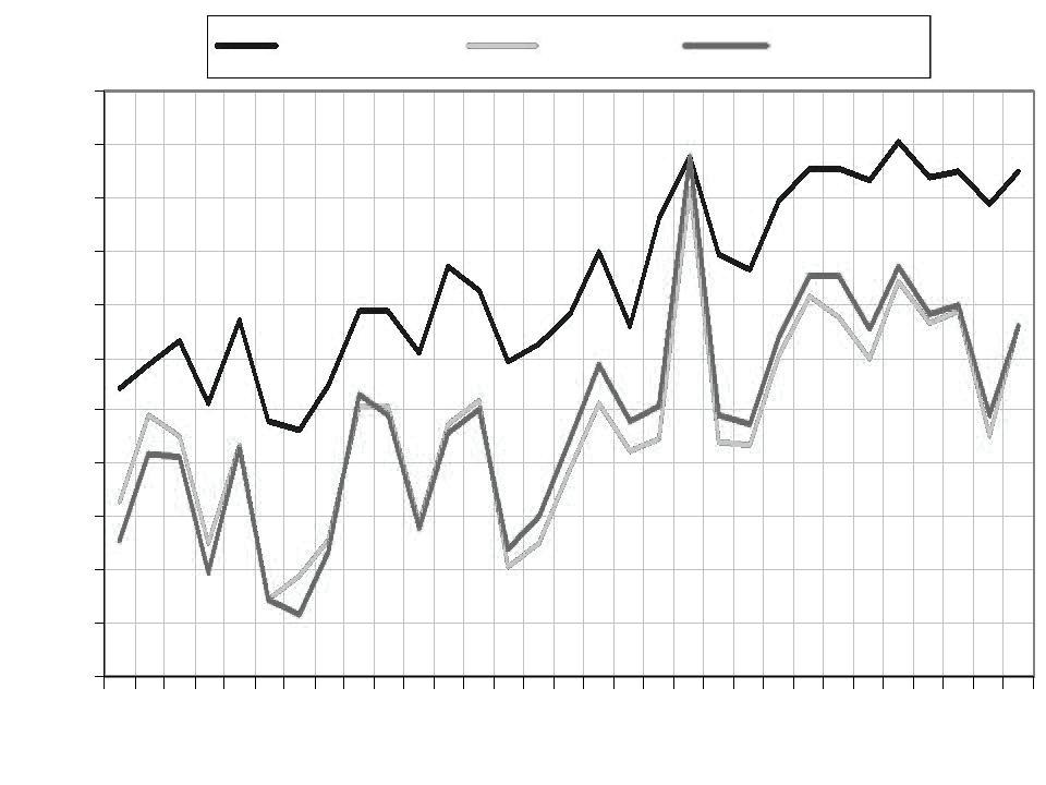
here have been numerous instances of NOAA meddling with the surface temperature record, in areas of the globe ranging from the Arctic to Australia to the U.S. Not only does NOAA exaggerate the warming rate, but the exaggeration also grows bigger over time, as can be seen by looking carefully at Figure 2.2

Figure 2.1: The Satellite Temperature Record

UAH Satellite-Based Temperature of the Global Lower Atmosphere El Niño Warming

Source: Spencer.57

that shows the diference between surface and satellite data constantly stretching – and this despite the fact that NOAA manages both the satellite and surface temperature programs.

A very recent reanalysis of the U.S. temperature record is a damning indictment of NOAA procedures. Using a new WMO-approved methodology for rating weather station siting, a study led by meteorologist Anthony Watts has found that published U.S temperature trends from 1979 to 2008 are twice as high as they should be, due mostly to NOAA’s erroneous upward adjustments to the data.63

NOAA, as we saw earlier, claims that their temperature adjustments obviate the need to correct for poor station siting. But the Watts study concludes that the corrected U.S. warming rate since 1979 ought to have been 0.16o Celsius (0.29o Fahrenheit) per decade for the best located stations, compared with the adjusted NOAA rate of 0.31o Celsius (0.56o Fahrenheit) per decade.64 Although the U.S. is only 2% of the world’s surface area, NOAA’s recent global warming rate – also

Figure 2.2: How NOAA Stretches the Temperature

Source: ICECAP 61 Theglobalsurfacetemperaturerecordis fromNOAA;62NOAAsatellitedatacompiledbytheUniversity ofAlabamainHuntsville(UAH)isthesameasinFigure2.1. Theverticalscaleshowsthetemperatureanomalyin oC.

0.16o Celsius (0.29o Fahrenheit) per decade – is undoubtedly high as well, as I discussed above.

Because urbanization goes all the way back to the 19th century, although it has accelerated in recent years, it’s highly probable that both IPCC and NOAA overestimates of the global warming rate since 1979 apply to the whole period from 1850 as well.

What this means is that the IPCC’s estimated global temperature increase of 0.8o Celsius (1.4o Fahrenheit) for the modern period is too high and should be trimmed by 25% – that is, by 0.2o Celsius (0.4o Fahrenheit) – down to 0.6o Celsius (1.1o Fahrenheit). he reduction called for is roughly consistent with the need to lower measured U.S. temperatures by about 0.13o Celsius (0.23o Fahrenheit), based on poor weather station siting, as I indicated before.

But even if reported global land and sea temperatures are inlated by 0.1o Celsius (0.2o Fahrenheit) to 0.2o Celsius (0.4o Fahrenheit), is that such a big deal? An exaggeration of this size in the global temperature uptick may not seem like much, but it’s enough to matter. he IPCC argument that natural variability alone cannot explain the observed rise in worldwide temperatures becomes a lot shakier if that rise has been overestimated by a few tenths of a degree, not to mention that the IPCC’s climate models then have much less validity.

Even at 0.1o to 0.2o Celsius (0.2o to 0.4o Fahrenheit), the exaggeration is, at the very least, poor science – poor science that has led the IPCC to make numerous unjustiiable predictions of disastrous consequences of global warming that await the Earth. Good science demands intellectual honesty, including correction of data for bias.

Disappearing Temperatures: he Hockey Stick

Much worse than a 0.1o to 0.2o Celsius (0.2o to 0.4o Fahrenheit) exaggeration in the modern temperature increase was the “hockey stick” scandal – an outrageous attempt by the IPCC to distort historical temperature data to suit its political agenda. he episode is well documented elsewhere but bears repeating here.

he scandal arose because of the IPCC’s need to validate its hypothesis about the connection between global warming and man-made CO2. We’ve seen how this hypothesis is based on similar upward trends in the modern temperature record and the CO2 level (Figure 1.1). If the hypothesis, and computer climate

models that depend on the hypothesis, are to hold up, then temperature and CO2 should track one another historically and not just for the last 160 years.

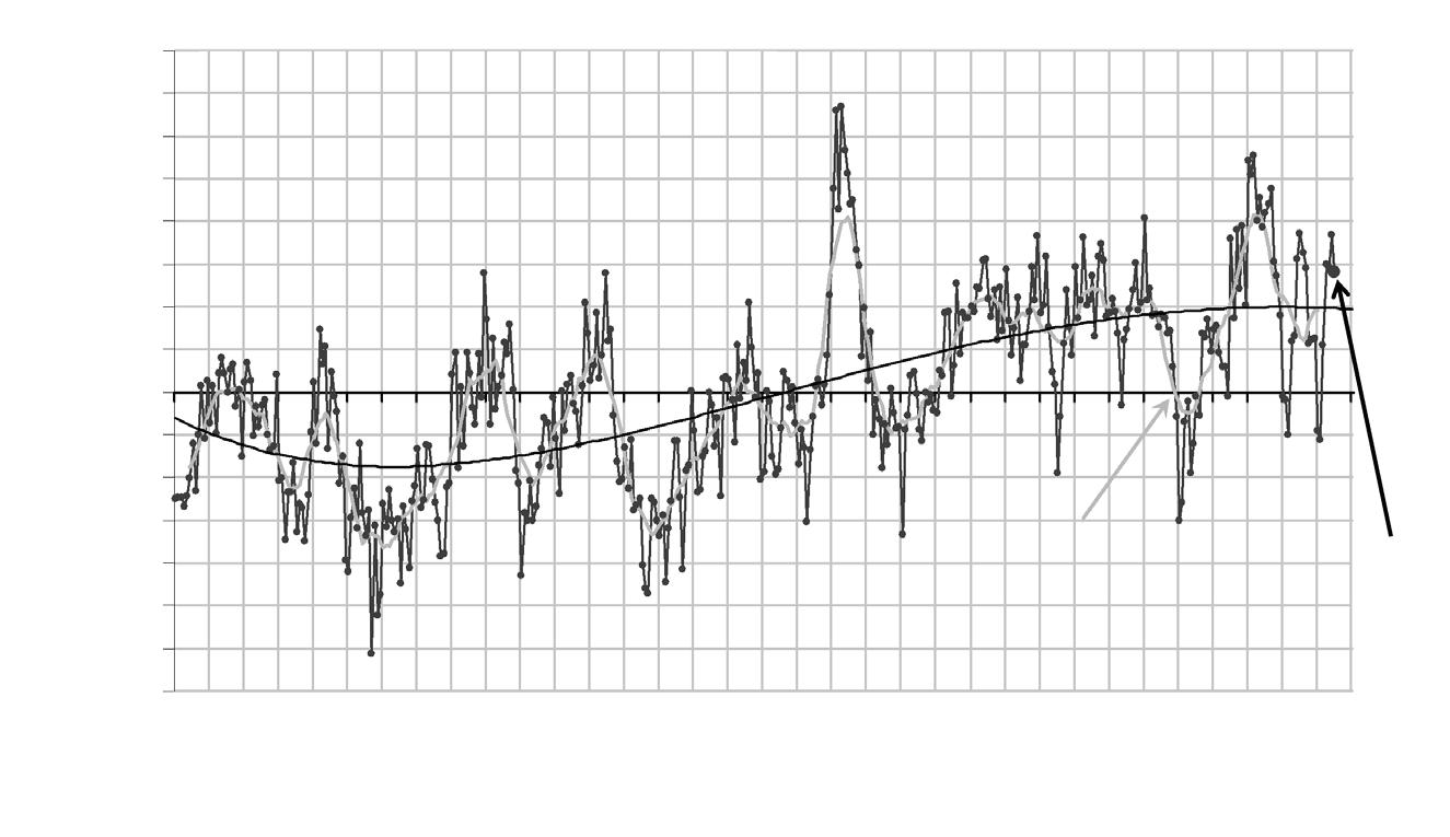
he diiculty with this need is that, over the last 2,000 years, the temperature and CO2 level don’t track (Figure 2.3). he temperature has luctuated, both up and down, but there has been almost no change in the CO2 concentration until modern times – the CO2 steady level problem referred to in Table 1.2.

How was this historical data obtained?

Measurement of temperature using scientiic thermometers goes back only to the early 18th century, and accurate determination of the CO2 level has been possible only for the last 55 years or so. Temperature and CO2 data for earlier periods come from so-called proxy methods, or indirect measurements using sources such as tree rings, ice cores, leaf fossils or boreholes.

Each of these proxy methods has its limitations. Although the most commonly used proxy for temperature is tree-ring data, some paleoclimatologists (climatologists who study the past) believe that tree rings are unreliable indicators. his is because the widths of tree rings respond not only to temperature, but also to other factors such as moisture and CO2. However, the data in Figure 2.3 were not based on tree rings.

he distinctly noticeable warm spell seen around the year 1000 is known to historians as the Medieval Warm Period, a time when warmer than normal conditions were reported in many parts of the world. he cool period centered around the year 1650 has been labeled the Little Ice Age and is also reported in various historical records. But there is no sign at all of these warming and cooling periods in the CO2 data for the same timespan, which is based on ice-core proxies.

As I said, this mismatch is a problem for the IPCC’s view of climate change. For the CO2 hypothesis to be correct, the temperature and CO2 level must go hand in hand, for all periods of time including the last 2,000 years.

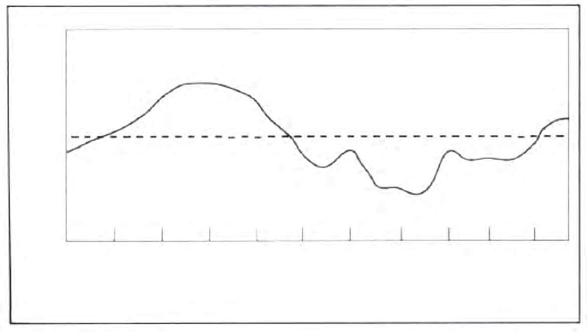
Oddly enough, the IPCC seemed unaware of this problem in its First Assessment Report in 1990 that showed a temperature graph for the last 1,000 years, with both the Medieval Warm Period and the Little Ice Age not only included, but clearly labeled (Figure 2.4).

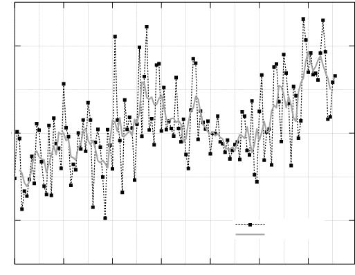
Yet the hird Assessment Report in 2001 told a radically diferent story. All of a sudden, the Medieval Warm Period and the Little Ice Age had disappeared! In their place was a fairly lat-looking graph (Figure 2.5) with few temperature ups

and downs until the beginning of the present climb around 1900 – a chart that now bore a remarkable resemblance to the modern CO2 record, looking like the shat and blade of a hockey stick on its side.

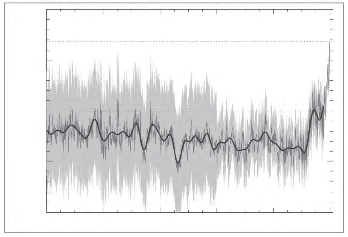
Sources: Temperature (showing 95% conidence intervals) – Loehle and McCulloch;65 CO2 – Intergovernmental Panel on Climate Change.66

Figure 2.3: The Last 2,000 Years of Temperature and CO2

GLOBAL WARMING FALSE ALARM

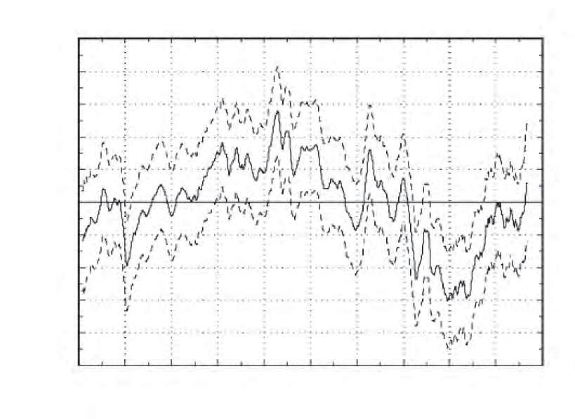
Hey presto! At a stroke, the IPCC solved its problem. he temperature record for the past 2,000 years indeed showed the same behavior as the CO2 level (and other greenhouse gases), and the IPCC could now proclaim that it was right about

Source: Intergovernmental Panel on Climate Change.69

Source: Intergovernmental Panel on Climate Change.68 Note that the horizontal time scale lines up approximately with Figure 2.4 above.

Figure 2.4: The IPCC’s View of History, 1990

Figure 2.5: The IPCC’s View of History, 2001 – The “Hockey Stick”

global warming being human-induced. If the panel was rewriting history at the same time, so be it.

he hockey stick graph was largely the work of Michael Mann, an IPCC author then at the University of Massachusetts, who published two papers in 1998 and 1999 reconstructing historical temperatures for the period from 1000 to 1980, based predominantly on tree-ring data. Intertwined with this pre-1980 proxy record was the 20th century thermometer record.67

Mann then conspired with his counterparts in the UK, who had produced similar but less wide-ranging graphs, to combine all the reconstructions into a convincing composite hockey stick for the IPCC’s 2001 report.68

Never mind that tree rings are considered an inaccurate proxy for past temperatures,70 nor that the 20th century thermometer record is exaggerated by the urban heat island efect, as I’ve just shown. he IPCC graph had an immediate visual and political impact. By doing away with the Medieval Warm Period and the Little Ice Age, the hockey stick not only vindicated what global warming alarmists had been saying, it also gave a boost to governments wavering on adoption of the UN’s 1997 Kyoto Protocol, which limits emissions of CO2.

Yet this apparent triumph for the IPCC’s global warming model was about to come crashing down around its ears, with the subsequent revelation that – yes, you guessed it – the IPCC and the hockey stick “team” were guilty of egregious data manipulation, of bending scientiic data for an ulterior motive.

Not well-known about the hockey stick is that the splicing together of treering and thermometer data was done simply because much of the tree-ring data indicates a temperature downturn ater about 1960, contrary to thermometer readings. A reconstruction of historical temperatures up until the present using tree rings alone would therefore not exhibit the characteristic hockey stick shape, since the upturned blade of the stick comes primarily from the modern thermometer data depicted in Figure 1.1.

To produce a hockey stick and get the alarmist message across, Mann and the IPCC deceptively retained the earlier tree-ring data but ignored the recent temperature downtrend in later data, substituting thermometer readings instead.71

Nonetheless, they did keep a tiny subset of tree-ring data that bucks the post1960 trend – ring widths from North American bristlecone pines, even though these are widely doubted to be dependable temperature proxies because of an

unexplained 20th century growth spurt. It was highly convenient, of course, that the bristlecone growth surge happened to reinforce the IPCC claim in the 1990s that global warming was accelerating. hat claim has turned out to be false.

But even though the mercury was rising in the late 1900s, playing fast and loose with the data isn’t acceptable science, as I said at the beginning of the chapter. Either you use all the tree-ring data, or none at all.

he Mann studies and the hockey stick were initially debunked in 2003 by Canadian statistician Stephen McIntyre and economist Ross McKitrick (coauthor of the urban heat island studies discussed earlier), who found that, apart from preferential data selection, Mann’s conclusions were based on faulty statistical analysis.72 In fact, McIntyre and McKitrick showed that they could almost always produce a hockey stick, even from completely meaningless random data In their words,

he particular “hockey stick” shape derived in the Mann proxy construction ... is primarily an artefact of poor data handling, obsolete data and incorrect calculation of principal components.73

he authors added that Mann’s studies were overly dependent on the tree-ring data from bristlecone pines. Omission of the bristlecone pine data, representing just one of over 100 data sets included in the original analysis, reinstates medieval warming and gives the lie to the IPCC’s assertion that our present warm trend is exceptional compared to preceding centuries.

In 2006, some ive years ater the publication of the IPCC’s report featuring the hockey stick, a team of statisticians appointed by the U.S. House Committee on Energy and Commerce found Mann’s statistical analysis to be “somewhat obscure and incomplete”, and the criticisms by McIntyre and McKitrick to be “valid and compelling”.74 he team also accused the IPCC of politicizing Mann’s work.

At almost the same time, the U.S. House Committee on Science, which had been charged by the National Research Council (NRC) of the National Academy of Science to report on temperature data for the last 2,000 years, came to similar conclusions. he NRC report states:

Large-scale surface temperature reconstructions yield a generally consistent picture of temperature trends during

the preceding millennium, including relatively warm conditions centered around A.D. 1000 (identiied by some as the “Medieval Warm Period”) and a relatively cold period (or “Little Ice Age”) centered around 1700. he existence and extent of a Little Ice Age from roughly 1500 to 1850 is supported by a wide variety of evidence including ice cores, tree rings, borehole temperatures, glacier length records, and historical documents. Evidence for regional warmth during medieval times can be found in a diverse but more limited set of records including ice cores, tree rings, marine sediments, and historical sources ...75

Despite this widespread denouncement of his work, Mann – who is a paleoclimatologist but not a statistician – has continued to argue for the legitimacy of the hockey stick graph. At one stage, he defended the absence of the Medieval Warm Period and the Little Ice Age from his temperature reconstruction by saying that these were local rather than global phenomena, and restricted to small regions of the Northern Hemisphere. he diiculty with this explanation is that there is ample historical evidence from around the world, including the Southern Hemisphere, of the existence of both climate periods.76

In 2008, Mann’s group published a new study reconstructing temperatures back to the year 700,77 based on a larger number of alternative proxies that weren’t tree rings than they had used in their earlier work.

In an apparent concession to critics, Mann (now at Pennsylvania State University) this time acknowledged the occurrence of medieval warming, although he still insisted that it didn’t come close in magnitude to our modern global warm spell. Mann even claimed in an interview that, far from being bent as the new reconstruction clearly shows, “the hockey stick is alive and well”.78

But hockey stick debunkers McIntyre and McKitrick were unsatisied, inding that the new Mann study contained further statistical laws, and that the group had failed to follow all the suggestions made by the NRC in its 2006 report.79

In an efort to rehabilitate the hockey stick, one of Mann’s UK colleagues published another study in 2008, utilizing Russian tree-ring data that appeared to show temperatures rising recently,80 just like thermometer data.  Unfortunately, that study too turned out to be lawed, relying heavily on a single freak tree (in

Yamal, Siberia) that doesn’t follow the downward trend of most tree-ring temperatures since 1960. his further attempt at deceit prompted McIntyre – who has become a self-appointed auditor of climate change claims – to call the lone tree “the most inluential tree in the world”.81

In contrast, a very recent Chinese study of tree rings over the last 2,485 years shows the occurrence of both the Medieval Warm Period and the Little Ice Age on the Tibetan Plateau, along with several earlier warm periods.82 he study is part of a major Chinese research project to better understand millennium-scale climate change.

What the IPCC will make of Mann’s recent work remains to be seen. Its 2007 Fourth Assessment Report grudgingly conceded that the hockey stick graph in the 2001 report was controversial, and that a more careful reconstruction of the temperature record does indeed show medieval warmth and chillier conditions during the Little Ice Age 83 But an article published in 2005 by a University of Oklahoma geoscientist, David Deming,84 leaves no doubt that in 2001, the IPCC was exploiting the hockey stick for its own ends.

Deming had established credibility with alarmists in the climate science community with an earlier paper, in which his analysis of borehole temperature data appeared to bolster the IPCC’s CO2 theory of climate change, although he concluded that natural variability could not be ruled out as a cause of warming either. he research was enough, nevertheless, to gain Deming admission to the alarmist club:

With the publication of the article in Science ... hey thought I was one of them, someone who would pervert science in the service of social and political causes. So one of them let his guard down. A major person working in the area of climate change and global warming sent me an astonishing email that said “We have to get rid of the Medieval Warm Period.”85

As we’ve seen, elimination of the Medieval Warm Period and the Little Ice Age was essential if the IPCC was to match up the temperature record and the CO2 level over the last 2,000 years (Figure 2.3), and thus substantiate its hypothesis that global warming stems from human activity. So Mann’s hockey stick curve, erroneous and deceptive as it is, must have seemed like a git from God.

TABLE 2.1: BAD IPCC SCIENCE – DATA mANIPULATIoN

The IPCC take on climate data

• Global warming is about 0.8 o Celsius (1.4 o fahrenheit) since 1850.

• The warming rate since 1979 has been 0.17 o Celsius (0.31 o fahrenheit) per decade, higher than ever before.

• Temperature and the CO 2 level in the atmosphere have always gone hand in hand, for all periods of time – past as well as present. This is required by the Co2 hypothesis.

WHAT’S WRONG WITH THIS DATA?

1. Global warming is exaggerated by 0.1

Celsius (0.2 o to 0.4o fahrenheit), because the IPCC has ignored a warming bias caused by artiicially high temperatures measured in urban areas. The bias is consistent with satellite data showing lower warming.

to 0.2

2. Both the IPCC and NoAA have inlatedtherecentwarming rate

3. NoAA boosts global warming by stretching the surface temperature record, which is steadily diverging from the temperature measured by NoAA satellites.

4. GISS magniies global warming by contracting past temperatures, rewriting the U.S. surface temperature record.

5. To match temperature to the Co2 level over the last 2,000 years, the IPCC rewrote history by eliminating the wellestablished medieval Warm Period and the Little Ice Age, creating the erroneous hockey stick graph.

Luckily for science, the world woke up to this particular case of IPCC corruption and the hockey stick – which I’ll revisit later in the chapter – is now largely discredited.

Disappearing Temperatures: GISS Rewrites the Past

Now you see it, now you don’t.

I’ve already discussed how far the IPCC and climate alarmists will go to keep alive their myth that man-made CO2 causes climate change. But the dishonesty goes beyond inlating temperature measurements and being deceitful with tree-ring data. In a blatant extension of the hockey stick saga, one of the major custodians of temperature data has begun tampering with the U.S. temperature record – and it looks like one of the others is following suit with global temperatures.

here are three principal guardians of the world’s temperature data, whose duties include analyzing the raw temperature data gathered from global weather stations. he three are NOAA and the NASA Goddard Institute for Space Science (GISS) in the U.S., and the UK collaboration between the Climatic Research Unit at the University of East Anglia and the Met Oice’s Hadley Centre (HadCRU).

he three organizations use diferent analytic approaches, and diferent subsets of the available temperature data, though there’s a lot of overlap so the three analyses are not completely independent. Nevertheless, the analyses play a key role in estimating how much global warming the planet has undergone.

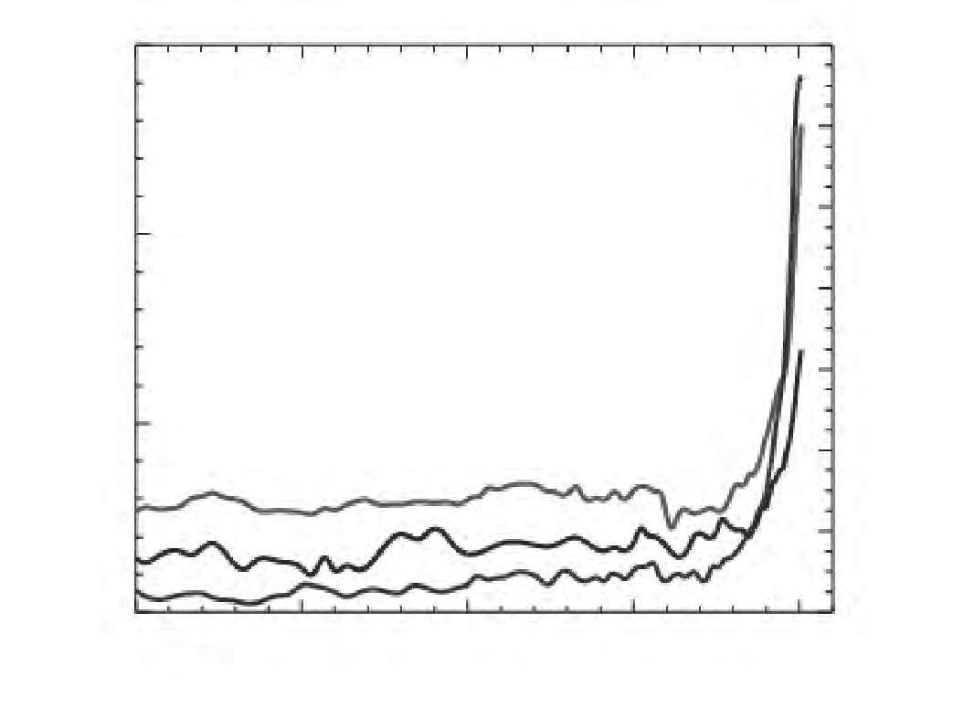
We’ve previously seen how NOAA boosts present-day global temperatures (Figure 2.2), in order to exaggerate the magnitude of global warming. GISS specializes in doing the same thing, mostly with past U.S. temperatures but in the reverse direction. hat is, GISS deliberately tamps down old temperature readings so as to make the past seem cooler than it really was.

Figure 2.6 reveals GISS at work on both fronts. In the period between 1999 and 2011, GISS not only meddled with U.S. temperatures from the 1930s – in particular, diminishing the record heat of 1934 – but also bumped up the readings from 1980 onwards.

Figure 2.6: How GISS Hikes Up Warming

he net efect, of course, is to make global warming in the U.S. appear more severe than it actually is. And while the original data showed 1934 to be 0.6o Celsius (1.1o Fahrenheit) hotter than 1998, which was another hot year, the revised version has 1998 warmer by about 0.1o Celsius (0.2o Fahrenheit)!88 In reality, most record high temperatures were set long ago (Table 2.2).

2.2: Worldwide Record High Temperatures89

GISS maintains that its recent revision of U.S. temperatures came only from changes to the raw temperature data made by NOAA, which in 2009 adopted a new method for correcting measured temperatures for bias, supposedly to reduce

Source: U.S. surface temperature record according to NASA GISS, in 1999 (let)86 and revised in 2011 (right).87

uncertainty in any climate trends deduced from the data.91 But it’s hard to believe that GISS and NOAA are acting in good faith, when every correction results in a steeper temperature increase from global warming, never a gentler one.

Even the UK’s HadCRU collaboration, which previously had the reputation for producing the most reliable temperature record (Figure 1.1) of the three organizations, has now started to play the same game. According to a 2012 report from the CRU, 2010 – and no longer 1998 – was the hottest year on record globally, allegedly based on a recent analysis of land temperatures that includes new data from weather stations in the Arctic.92

I’ve now looked at three separate examples of how the IPCC and its allies have abandoned any pretense of playing by the scientiic rules in arriving at their position that humans have caused global warming – by ignoring bias in the modern temperature record, misrepresenting the historical temperature record, and doctoring temperatures over the last century. If submitted as part of a science thesis by a PhD student in a reputable institution, any one of these eforts alone would be enough to fail the student.

But there’s more. We’ll see in the next section that the IPCC and climate change alarmists not only thumb their noses at accepted procedures for handling scientiic data, but they also stoop to shady and corrupt practices in presenting and publishing that data.

CORRUPTION AND FRAUD

Biased from the beginning toward its belief in man-made global warming, the IPCC – along with CO2 warmists in the scientiic establishment and the media – has spared no efort in attempting to suppress contrary scientiic evidence and to stile the views of critics. his line of attack has extended to brazen dishonesty as we’ve just seen, and even to making fraudulent claims.

Suppressing Evidence: Climategate

A slew of scandalous revelations, many intimately connected to the infamous hockey stick curve, recently came to light when thousands of embarrassing emails from the Climatic Research Unit (CRU) at the UK’s University of East

Anglia were leaked onto the Internet – irst in November 2009, then again late in 2011. It’s not known to this day whether the incidents, known as Climategate, were the work of an outside hacker or an inside whistle-blower at the CRU.

But the private emails between several of the world’s top climate scientists, both at the CRU and in the U.S., reveal numerous instances of the Climategate perpetrators conspiring to suppress evidence, simply to buttress the faulty hypothesis that climate change comes from human activity.

he misdeeds include extensive data manipulation; subterfuge to keep temperature data and computer codes from being released to outside researchers who wanted to perform independent analyses; destruction of records; and interference with the peer review process to prevent contrary scientiic papers from being published. All in the name of the CO2 theory of global warming and its assertion that temperatures today are the highest in more than 1,000 years.

I’ll return to the issue of peer review later. Here we’ll take a look at just three of the many scientiic transgressions committed by the Climategate gang.

Towering over all the revelations is the shameful efort to “hide the decline” in recent global temperatures derived from tree-ring data – an efort that was part of the deceptive reconstruction of historical temperatures involved in creation of the now discredited hockey stick.

he machinations began in September 1999 with the meeting of IPCC lead authors to discuss the irst drat of the hird Assessment Report. Shortly ater this meeting, in an email to his UK colleagues, hockey stick architect Mann expressed concern about the downturn in temperatures shown by nearly all the tree-ring data ater 1960, which didn’t it with the upsweep of the hockey stick: he key thing is making sure the series are vertically aligned in a reasonable way. I had been using the entire 20th century, but in the case of Keith [Brifa]’s, we need to align the irst half of the 20th century with the corresponding mean values of the other series, due to the late 20th century decline.93

Here Mann is talking about the composite temperature reconstruction that was to appear in the IPCC report, based on both the hockey stick and similar reconstructions by his UK associates. His concern over the visibility of the decline in tree-ring temperatures got the others’ attention. Only two months later, CRU chief Phil Jones announced to the group:

I’ve just completed Mike [Mann]’s Nature trick of adding in the real temps to each series for the last 20 years (ie from 1981 onwards) and from 1961 for Keith [Brifa]’s to hide the decline.94

In no uncertain terms, this email exposes the deliberate deceit behind the hockey stick. he “trick” that Jones refers to – and seems proud of – was originally employed by Mann in his 1998 paper in the journal Nature, in which thermometer measurements were substituted for the bulk of the post-1980 tree-ring data, but the earlier tree-ring data was retained.67 Although normal scientiic practice would have been to draw attention to this procedure in the paper and to justify it, Mann chose to hide the deception by saying nothing.

he silence about hiding the decline continued in the IPCC hird Assessment Report in 2001, just as Jones’ email had foreshadowed. And even in the Fourth Assessment Report in 2007, suppression of the post-1960 data71 is only mentioned in passing, as part of a general discussion on the limitations of tree rings as a proxy.83

he incompatibility of the Medieval Warm Period with the hockey stick concept has been an ongoing thorn in the IPCC’s side. his is evident in a 2003 email from Mann, in which he wrote:

I think that trying to adopt a timeframe of 2K [2000 years], rather than the usual 1K [1000 years], addresses a good earlier point that Peck [Jonathan Overpeck] made with regard to the memo, that it would be nice to try to “contain” the putative MWP [Medieval Warm Period], even if we don’t yet have a hemispheric mean reconstruction available that far back.95

Use of the word “putative” signiies that the Climategate gang was intent on minimizing the Medieval Warm Period, even when there wasn’t enough data to back up their cratiness. Climate scientist and IPCC lead author Jonathan Overpeck, who is quoted here, is rumored to be the source of the email mentioned earlier in the chapter on completely eliminating the Medieval Warm Period from the historical record.

You don’t need to be a scientist to know that the data manipulation described in these emails is shamelessly dishonest. Although the hockey stick was eventually

debunked, it is only the Climategate emails that have uncovered the true extent of the fraud involved.

A second major transgression concerns the important scientiic issue of reproducibility. he scientiic method requires that all observations and results of analyses be repeatable by others – a safety measure to guard against bias. Because so much of the hockey stick saga seemed questionable, McIntyre and several other skeptics decided to ask for copies of the proxy data and computer codes used by Mann and his collaborators, so they could perform independent analyses of the same data and thus verify or invalidate the conclusions.

While requests of this type are welcomed in most scientiic circles, the Climategate conspirators put up a near impenetrable wall of resistance. Mann’s group blocked the move at every turn, making it much more diicult than it should have been for McIntyre and McKitrick, who originally debunked the hockey stick graph in 2003, to obtain all the detailed information they sought on the hockey stick calculations.

Annoyed by McIntyre’s persistence, Mann responded to a 2004 email from Jones by stating:

I have no idea what he [McIntyre]’s up to, but you can be sure it falls into the “no good” category. … I would not give them anything. I would not respond or even acknowledge receipt of their emails. here is no reason to give them any data, in my opinion, and I think we do so at our own peril!96 Mann evidently felt they had something to hide, other than the decline.

Concerted eforts by climate change alarmists to discredit McIntyre altogether, such as trying to link him to the fossil fuel industry, a favorite alarmist tactic, failed. Instead, a resolute McIntyre explored how to obtain what he still needed through the U.S. Freedom of Information Act (FOIA), a tool frequently used by investigative reporters. his move greatly rattled Jones in the UK, who wrote to Mann in February 2005, saying:

he two MMs [McIntyre and McKitrick] have been ater the CRU station data for years. If they ever hear there is a Freedom of Information Act now in the UK, I think I’ll delete the ile rather than send to anyone. … We also have a data protection act, which I will hide behind.97

And, just three weeks later, to three others:

I’m getting hassled by a couple of people to release the CRU station temperature data. Don’t any of you three tell anybody that the UK has a Freedom of Information Act !98

So not only were the Climategate gang scheming to suppress data, but they also felt above the law in concealing their wrongdoing. Despite the CRU being a publicly funded institution and therefore legally obliged to retain records of its work and to make them available for scrutiny, Jones had no qualms about deleting a computer ile or doing anything else necessary to prevent CRU records from being released. And this is far from being the only example, either in the UK or the U.S., of iles or emails being deleted to prevent their public disclosure.

Above all, the Climategate perpetrators were intent on keeping as much as possible of the hockey stick data and computer codes out of McIntyre and McKitrick’s hands. In the end, however, the law prevailed and the hockey stick team was forced to hand over the remaining pieces of data and code.

But, no doubt wondering what additional errors McIntyre and McKitrick would discover in the team’s tree-ring analysis, a recalcitrant Mann complained in 2006 that he didn’t see “why you should make any concessions for this moron [McIntyre]”.99 McIntyre had just accused other hockey team members of “juvenile behavior” in obstructing his FOIA requests. As I discussed before, McIntyre and McKitrick did indeed go on to unearth laws in a further Mann study.77, 79

Alarmist apologists have attempted to defend the work of the hockey stick team. However, the science itself aside, secrecy and unwillingness to share data – in both of which the central igures in Climategate excelled – have no place in proper scientiic methodology.

A third instance of suppression of evidence that the Climategate emails made public involves allegations of fraud, in connection with the urban heat island efect. he allegations were made from 2007 to 2009 against climate scientist WeiChyung Wang, who is a professor at the State University of New York at Albany, by former UK inancial analyst Douglas Keenan.100

he alleged fraud concerns two 1990 research papers coauthored by Wang, in which a comparison was made between temperatures gathered at both urban and rural weather stations in China over the years 1954 to 1983.101, 102 he lead author on the second paper was none other than the CRU’s Jones.

-40-

Keenan accused Wang of fabricating more than half the station histories – that is, making up the raw temperature data – as well as lying about changes in station location. A statement in both research papers that there were few station moves, which afect temperature measurements, was shown by Keenan to be false, since many of the stations moved multiple times during the 30 years of the study. One station had ive diferent locations from 1954 to 1983, some of the locations being as much as 41 kilometers (25 miles) apart.103

By Keenan’s estimate, the station moves could have afected the measured Chinese temperatures that were used in the two studies by as much as 0.4o Celsius (0.7o Fahrenheit),100 which is a substantial portion of the average temperature increase worldwide from global warming during the study period.

he paper with Jones as lead author concluded, partly from the allegedly fabricated data, that urbanization in China has no signiicant efect on measured temperatures 102 his particular study is highly important, as it was cited by the IPCC in its 2007 report as evidence that the urban heat island efect is negligible,104 along with its own fabricated evidence to be discussed in the next section.

he Climategate emails strongly hint that Jones was complicit in covering up the fraud. Perhaps the most telling sign that he was more than just an innocent coauthor of Wang was a 2010 article about the case in the UK’s he Guardian – a newspaper known more for attacking climate change skeptics such as Keenan than defending them.105

In an internal CRU email sent in February 2007, responding to yet another FOIA request from climate auditor McIntyre, asking for the original Chinese data, Jones wrote, “I don’t really see this as an FOI request. I am really loath to send them the data even if I could ind it.”106 Jones had told McIntyre previously that supplying the data would be “too burdensome”. In March 2007, Keenan requested the same Chinese data.

he requests prompted hockey stick creator Mann to weigh in shortly aterwards, advising Jones that:

his is all too predictable. his crowd of charlatans is always looking for one thing they can harp on … he last thing you want to do is help them by feeding the ire. Best thing is to ignore them completely.107

he Climategate gang was up to its old tricks again, although the obstruction was once more in vain. Ater Wang agreed to supply the questionable station data, Jones felt obliged to pass it on to Keenan and McIntyre. But Jones and his colleagues were taken aback when Keenan then made his fraud allegations, which are still unresolved.

However, Jones recently reversed himself. In a new study of Chinese temperatures, he reported not only that a strong urban warming efect does indeed exist in China, but also that urban warming caused the China-wide temperature rise between 1951 and 2004 to be overstated by a whopping two thirds.108 In an obvious attempt to distance himself from the fraud charges, Jones did not include Wang among his coauthors on the new study.

hese three examples of corruption exposed by Climategate are just the tip of the iceberg. Many more can be found in the voluminous emails, which have been dissected in numerous blogs and books. he obstructive behavior has been called “climate tribalism” by Judith Curry, a leading climatologist who is chair of the School of Earth and Atmospheric Sciences at the Georgia Institute of Technology, and one of the few voices of reason among nonskeptics.109

Because of the public outcry over Climategate, there have been several oicial investigations into the scientiic misconduct exposed by the emails. he oicial inquiries were conducted in the UK (three separate investigations of the CRU), the U.S. (of Michael Mann), and the Netherlands (of the IPCC).

But just as we might expect, a majority on the investigating panels consisted of either scientists who were advocates of the man-made global warming theory or, in the case of Mann, Pennsylvania State University personnel – who were more interested in protecting Mann for his research funding prowess than in looking into the charges against him. None of the panels interviewed any critics of the Climategate ofenders.

So it was no surprise, at least to climate change skeptics, when the oicial investigations almost completely whitewashed the fraudulent and obstructive behavior being investigated. Even a columnist normally supportive of the alarmist view found the reports “At best … mealy-mouthed apologies; at worst … patently incompetent and even wilfully wrong.”110

he only concession made to critics was by one of the UK reviews that chastised the CRU and the University of East Anglia for showing “a consistent pattern of failing to display the proper degree of openness”.111

Cooking up Evidence

Beyond the deception, obstruction and cover-ups revealed by the Climategate emails is yet another example of fraud by the IPCC – this time involving the creation of ictional evidence to prop up a fallacious argument about urban heat islands.

As discussed earlier in this chapter, the IPCC’s 2007 report minimizes the inluence of urbanization on recorded temperature data. Imagine its astonishment, then, when upstarts McKitrick and Michaels published their detailed statistical study showing that the urban heat island efect accounts for just over a half of the measured temperature increase on land due to global warming.51, 112

Perhaps in the hope of silencing any public comment by McKitrick, the IPCC had made him an external reviewer for that part of the report. heir eforts backired, however, as McKitrick not only submitted extensive comments in support of the conclusions he and Michaels had reached, but also struck back openly at the IPCC when those comments were passed over.113

In explaining why he accepted the IPCC’s invitation to serve as a reviewer, McKitrick says:

Contamination of surface climate data is a potentially serious problem for the IPCC. Conclusions about the amount of global warming, and the role of greenhouse gases, are based on the assumption that the adjustment models work perfectly ... the core message of the IPCC hinges on the assumption that their main surface climate data set is uncontaminated. And by the time they began writing the recent Fourth Assessment Report, they had before them a set of papers proving the data are contaminated 114

he IPCC report dismisses the McKitrick and Michaels study with the false statement that most global temperature measurements have already been adequately adjusted for urbanization, and that only a very small additional correction is necessary. McKitrick wrote a lengthy criticism of this opinion, backed

up by strong evidence to the contrary from the study, during the writing of the IPCC report.

What happened next is astounding, but typical of how the IPCC operates. Confronted with published evidence from one of their own reviewers that the heat island efect contaminates global temperatures, they trivialized the evidence with the conjecture that urban warming can be chalked up to entirely natural causes. In publicly available comments on the report’s second drat, the IPCC authors state that the urban heat island efect is insigniicant and that any urban warming comes from “...strengthening of the Arctic Oscillation and the greater sensitivity of land than ocean to greenhouse forcing owing to the smaller thermal capacity of land.”115

his preposterous claim is complete nonsense. he Arctic Oscillation is a wind circulation pattern that afects long-term weather trends in the Arctic, but has absolutely nothing to do with the heat island efect from urban areas. And the comparison of land to ocean is irrelevant since McKitrick and Michaels only studied temperatures over land.

But the IPCC didn’t stop there. Referring to the strong connection that McKitrick and Michaels found between temperatures and local economic activity, the inal version of the report declares:

However, the locations of greatest socioeconomic development are also those that have been most warmed by atmospheric circulation changes (Sections 3.2.2.7 and 3.6.4), which exhibit large-scale coherence. Hence, the correlation of warming with industrial and socioeconomic development ceases to be statistically signiicant.50

Here the IPCC acknowledges the correlation between warming trends and socioeconomic development, meaning industrialization and urbanization, but dismisses the correlation as a mere coincidence due to unspeciied “atmospheric circulation changes”. his is more of the Arctic Oscillation gobbledygook that the IPCC authors invoked earlier in the report writing process, since the two cited sections of the report say nothing at all about industrial or urban development.

However, the most outrageous comment is the second sentence in the excerpt above, maintaining that McKitrick and Michaels’ evidence for a deinite correlation between elevated temperatures and urbanization is statistically insigniicant.

McKitrick has since demonstrated in a further study, which speciically includes four major atmospheric circulatory (wind) patterns, that exactly the opposite is true – that is, the correlation is indeed statistically signiicant, and measured temperatures are strongly tied to urbanization.116

he IPCC’s claim to the contrary is a lagrant abuse of science and scientiic methodology. Not only did the UN panel reject perfectly sound scientiic evidence in McKitrick and Michaels’ previous studies, but they did so on the basis of nonexistent counterevidence from wind patterns. In McKitrick’s words, this amounts to “making stuf up” and constitutes a “plain fabrication” by the IPCC.113

Peer Review as a Weapon

One of the favorite tactics of global warming alarmists is to wield the timehonored tradition of peer review in scientiic publishing as a weapon against skeptics. While this may be less outrageous behavior than some of the other abuses I’ve just described, it’s still corrupt.

he tactic takes several forms. In a common line of attack, alarmist climate scientists band together to write negative reviews of a skeptical research paper submitted to a scientiic journal, oten purely on the grounds that the paper contradicts the status quo, which is dominated by the man-made CO2 hypothesis, and therefore couldn’t possibly be worthy of publication.

Alternatively, when there’s little to criticize in the manuscript, alarmist reviewers pressure the journal editor to throw it out because it’s not written by a member of the alarmist club. If the editor doesn’t comply, and continues to accept papers from skeptics, the alarmists move to have the editor ousted.

he Climategate emails provide ample insights into both these strategies. As a result of the clamor over the hockey stick, paleoclimatologists – the tree-ring folk – went to great lengths in trying to keep contrary papers from seeing the light of day. Many skeptical climate scientists have experienced lengthy delays in publication of their manuscripts, or have had to submit them to obscure journals, because normal publication was thwarted by alarmists.

At the very least, the Climategate gang wanted to exclude skeptics from IPCC reports. Jones conided to Mann in 2004:

Ican’tseeeitherofthesepapersbeinginthenextIPCCreport. Kevin [Trenberth] and I will keep them out somehow – even if we have to redeine what the peer-review literature is !117

Alarmists have been successful in orchestrating the removal of “ofending” journal editors who dare to accept skeptical papers. In a 2003 email to a large group of paleoclimatologists and others, climate scientist Tom Wigley discussed a paper he didn’t like that had been published in 2002 by skeptical climatologist Michaels in the journal Climate Research. Wigley and another reviewer had written negative reviews of the manuscript and had recommended rejection, but the paper appeared in print because three other reviewers gave it the thumbs-up.

Piqued, Wigley wrote:

I suspect that de Freitas [a Climate Research editor] deliberately chose other referees who are members of the skeptics camp. I also suspect that he has done this on other occasions. How to deal with this is unclear, since there are a number of individuals with bona ide scientiic credentials who could be used by an unscrupulous editor to ensure that ‘anti-greenhouse’ science can get through the peer review process.118

Clearly, Wigley thought – like many other alarmists – that any papers questioning the CO2 explanation of global warming should never be published, regardless of their scientiic merits.

Chris de Freitas stayed on as an editor at Climate Research, in spite of an ad hominem campaign by the Climategate gang to have him both removed from his editorial position and even ired from his university job.119, 120 Nevertheless, the Climategate conspirators made so much noise about another skeptical paper published in the journal in 2003 that not only was its editor-in-chief forced to resign, but four other editors also let.121 Among other claims, the paper in question maintained that the Medieval Warm Period was warmer than today.

Intimidation of editors worked again at a diferent publication two years later, by which time the frustration level among paleoclimatologists had risen further. Shocked that the mainstream scientiic journal Geophysical Research Letters (GRL), which publishes a large number of alarmist papers on climate change, had

just given the green light to one of McIntyre and McKitrick’s studies debunking the hockey stick,72 Wigley emailed his colleagues in 2005, saying: his is truly awful. GRL has gone downhill rapidly in recent years. … If you think that Saiers [GRL editor] is in the greenhouse skeptics camp, then, if we can ind documentary evidence of this, we could go through oicial AGU [American Geophysical Union] channels to get him ousted. Even this would be diicult.122

Despite Wigley’s reservations, the editorship of GRL did indeed change hands later that year. If they couldn’t convince everyone that the hockey stick was real, the hockey team could at least control the world of climate science publishing.

Yet another editorial resignation over peer review occurred as recently as 2011, at the relatively new journal Remote Sensing. In this case, the journal had published a controversial paper on climate sensitivity (see Chapter 4) by well-known skeptical climatologist Roy Spencer and a coauthor, who used satellite measurements to challenge the reliability of computer climate models.123

Because computer models are at the heart of climate change hysteria, alarmists rose up en masse and complained, both to the journal and in public, about the perceived failure of peer review in allowing a skeptical paper to penetrate alarmist early warning defenses.124 Within a month, Remote Sensing editor Wolfgang Wagner stepped down in order to appease his critics.

But Wagner’s disingenuous resignation editorial, which has been described as “eerily reminiscent of past recantations by political and religious heretics”,120 makes it clear it was skeptics, and not the peer review process itself, that were the actual alarmist target:

herefore, from a purely formal point of view, there were no errors with the review process. But, as the case presents itself now, the editorial team unintentionally selected three reviewers who probably share some climate sceptic notions of the authors.125

Just keep the skeptics out of the scientiic literature and the CO2 theory can reign supreme.

IPCC Dirty Tricks

he IPCC as an organization is no less corrupt than the Climategate ofenders. And nowhere is corruption in the IPCC more visible than in the review process by which the conclusions of its climate scientists become part of the panel’s published reports – reports that constitute the bible of climate change alarmists

But just as bias toward human-induced global warming is built into the IPCC’s original mandate, politicization and corruption of the report review process are, amazingly enough, inherent in the panel’s working principles. hese principles state:

Changes (other than grammatical or minor editorial changes) made ater acceptance by the Working Group or the Panel shall be those necessary to ensure consistency with the Summary for Policymakers or the Overview Chapter.126

In other words, the science should be modiied if needed to conform to the Summary and Overview, which get written irst! hat’s like asking a jury to rubber stamp a verdict that the judge has already decided on. In the inancial world, it’s called cooking the books.

A disturbing example of corruption in the IPCC reviewing process occurred during preparation of the Second Assessment Report back in 1995, when the IPCC was trying very hard to establish the concept of a “discernible human inluence” on climate. his has been described in detail elsewhere, so I’ll only dwell on it briely here.

In order to link global warming with man-made CO2 and identify a climate change signal, the IPCC attempts to apply a technique called “ingerprinting”, whereby geographic and temporal patterns of higher temperatures are matched to the predictions of computer climate models.

But the 1995 IPCC claim to have successfully identiied a human ingerprint on global climate was demonstrably false, because it was based on selective use of temperature data. When all the data were examined as a whole, the case for a human CO2 signature in our climate was found to be very weak.

hat caused a considerable ruckus at the report review stage. In a rare display of honesty by the IPCC, the drat of the report disputed the success of ingerprinting and actually questioned the evidence for any human efect on climate. he drat included as many as 15 statements relecting these views.

In the inal version, all the statements had gone, being replaced by quite diferent language implicating greenhouse gases such as CO2 in global warming, and claiming that, for the irst time, evidence now existed for a human inluence on climate.127 his claim was a sea change in the public declarations of the IPCC, which up to then had made only tentative declarations about human-induced climate change, and played a major role in subsequently shiting public opinion toward the alarmist viewpoint.

But the drastic changes from the drat version of the report had all been made surreptitiously, by a small group of about six authors for that particular chapter, including lead author Ben Santer – without the other authors or any reviewers even being consulted. he alarmists had won their irst battle against the skeptics, inside the IPCC itself.

Frederick Seitz, an eminent physicist and past president of both the National Academy of Sciences and the American Physical Society, wrote at the time that he had never witnessed “a more disturbing corruption of the peer-review process” than the events that led to the IPCC report, and accused the IPCC of tampering with science for political purposes.128

Even the prestigious journal Nature, while supportive of the IPCC’s stance on global warming, castigated the panel in an editorial, saying that: IPCC oicials claim ... the revisions [were made] in particular to ensure that it conformed to a ‘policymakers’ summary’ of the full report ... But there is some evidence that the revision process did result in a subtle shit ... that ... tended to favour arguments that aligned with the report’s broad conclusions.129

he IPCC, in line with its corrupt working principles, had turned the review process upside down and had replaced perfectly good science with what had already been written in the report summary. One of the authors of the altered chapter basically admitted as much in a later attempt to defend the IPCC’s position, saying that the whole report was unquestionably “fraught with political signiicance”.130

Little has changed at the IPCC since then. However, the recent investigation of the IPCC in the wake of Climategate did address a number of issues, including assessment report review.

GLOBAL WARMING FALSE ALARM

TABLE 2.3: BAD IPCC SCIENCE – CoRRUPTIoN AND fRAUD

Areas of IPCC corruption

• The historical temperature record.

• Release of data and computer codes for publicly funded climate research.

• The effect of urbanization on global temperatures: two separate cases, one involving alleged fraud.

• Peer review in climate science publishing, including intimidation of j ournal editors.

• The IPCC’s internal process for reviewing climate assessment reports.

WHAT’S WRONG WITH THIS SCIENCE?

1. IPCC authors dishonestly conspired to “hide the decline” in recent temperatures derived from tree-ring data, as part of the deceitful skewing of historical temperatures to produce the discredited hockey stick curve.

2. The Climategate gang willfully obstructed FOIA requests for proxy data and computer codes used to create the hockey stick. There is evidence in the Climategate emails that iles and email records were destroyed.

3. Formal charges of fraud have been made against an IPCC climate scientist in connection with urban warming, for allegedly fabricating Chinese temperature data and lying about weather station histories. The Climategate perpetrators may have been complicit in a cover-up

4. The IPCC dismissed sound statistical evidence that urbaniz ation artiicially inlates global temperatures, by using double-talk and by citing nonexistent counterevidence – which led to accusations of fabrication against the IPCC by the authors of the statistical study.

5. The Climategate offenders have interfered with the peer review process, and orchestrated the removal of journal editors, in order to prevent the publication of scientiic papers contrary to the Co2 theory of global warming.

6. IPCC principles require the science in its reports to conform to the policymakers’ summary, a political document that is often written before the body of the report. And in the 2007 report, 30% of the scientiic sources were not peer reviewed

Among the inquiry’s recommendations were that the process for approving the Summary for Policymakers be revised, in order to reduce political interference with the scientiic results; and that IPCC review editors should exercise their authority to ensure that “properly documented alternative views” receive due consideration, and that “genuine controversies are adequately relected in the report”.131

he inquiry also found that the IPCC needs to strengthen and enforce its procedures for citing unpublished and non-peer-reviewed literature in its reports. his recommendation was a response to a survey revealing that a staggering 30% of the so-called scientiic sources cited by the alarmist IPCC in 2007 were not peer-reviewed at all,132 but included newspaper articles, reports from lobbyists, and brochures – despite the eforts of the Climategate gang to keep any skeptical papers on climate science in the non-peer-reviewed category.

But it remains to be seen how seriously the IPCC will take these indings. he organization’s existing review process is highly compromised from years of abuse, and fundamental reforms need to be implemented.

Chapter 3: Computer Snake Oil

Alarmist climatologists, when attacked by skeptics in other scientiic disciplines for promoting belief in man-made global warming, are fond of hiding behind their so-called expertise in climate science. We’re the experts, they declare – so only they are qualiied to pass an authoritative opinion on climate change.120

While not being an expert in a particular ield doesn’t disqualify a scientist in another ield from evaluating the evidence and passing an opinion, you need to ask yourself in this case whether the climate scientists who claim to be experts really are. It’s no secret, but it’s not widely known that their “expert” opinions are based entirely on theoretical computer models of the climate.

Computer climate models are also the foundation for the gloom and doom about CO2 and global warming preached by the IPCC. However, as we’ll see, the IPCC’s computer models are a poor imitation of reality and have made many predictions that have simply turned out to be wrong.

Because computer models are central to the climate change debate, the whole of this chapter is devoted to them.

IT’S ONLY A MODEL

Computer models can be very powerful tools. One area where computational models are particularly useful is the design and engineering of complex technological marvels such as cars, airplanes, or computer chips. For all of these, the underlying science is well known and the assumptions behind the models have been thoroughly tested.

Models don’t do as well when the computation is unable to mirror the reality of a complex system. his happens when there are gaps in our knowledge of the model’s infrastructure, and we have to use guesswork to ill in the gaps. Now we can no longer be certain about what the model tells us.

Computer climate simulations are only as reliable as the assumptions that the computer model is built on: “garbage in, garbage out”, as sotware engineers like to say. Just as scientiic hypotheses need to be veriied experimentally before they can be conirmed – a requirement that the IPCC actually recognizes133 – so do any educated guesses made in a computer calculation.

One of the biggest defects in the IPCC’s argument for human-caused global warming is that its theoretical climate models are chock-full of untested assumptions. hey include conjectures about basic elements of the climate system, such as clouds and precipitation; about the contribution, largely ignored, of natural cycles to current high temperatures; and about the physical processes that control the response of the Earth’s climate to tiny additions of CO2, a response much exaggerated in the models.

I’ll discuss these and other assumptions as we go through the book. he real problem is that many of the assumptions are undergoing testing right now, in an ongoing experiment that may not be complete for another 50 or 100 years. Alarmists and the IPCC say we can’t aford to wait that long for the results, so our only choice is to rely on computer modeling

Nevertheless, there is abundant evidence that the IPCC’s computer models do not accurately simulate even the present-day climate, let alone the future or the past. Many of the predictions made by these models about current climatic conditions have been dead wrong, and the only reason that climate models can “hindcast” the historical record is that they are arbitrarily adjusted to it the historical data.

Even though computer simulations can be useful, it’s easy to become carried away with their possibilities and to inlate the importance of their predictions.

Something I’ve noticed in my own research is that, while some features of any experimental results obtained in the real world can be reproduced by theoretical computer calculations, other features typically can’t. And computational models tend to exaggerate the magnitude of trends in the actual data. he reason is simple: computer models depend on assumptions, and it’s next to impossible to

make all the right assumptions. here are just too many unknowns that can’t be measured or tested.

It’s not very diferent with climate models. Some of the models are very elaborate and can predict all sorts of climatic variables in great detail – so much so that we can be awed by the model itself, by the sheer calculating power at our ingertips. I’ve certainly experienced that feeling.

But a model is just a model. Even though the computational power of current supercomputers used for climate modeling is more than a million times greater than what was available in 1970, when computing was in its infancy, that doesn’t change the fact that the models are constrained by their underlying assumptions. All the computing speed in the world doesn’t make up for lack of understanding.

he 2008 Wall Street meltdown is a painful reminder of this. Although the reasons for the U.S. inancial crash and the subsequent Great Recession are numerous, there’s no doubt that computer models played a role, since it was computer simulations that had been routinely used to evaluate risk by the investment community. If the models had better represented reality, or if bankers had been more aware of the limitations of computer modeling, perhaps the inancial crisis wouldn’t have been as bad as it was.

Another notorious example, from the engineering ield, is the Millennium Bridge in London. It was only ater the footbridge was built, and people walked on it for the irst time, that unexpected swaying was felt by walkers, causing the bridge to be promptly closed for design modiications. he engineers realized they had created what is known as a resonant structure, a well-understood phenomenon that could have been avoided if they had made correct assumptions in their computer models of the bridge.

Climatologists defend their theoretical computer models by saying the models are the only handle we have on the climate. hat is true, unless we’re prepared to wait several decades until we have some more deinitive measurements. But that doesn’t mean the models are right. I certainly wouldn’t want to ly on an airplane designed by the engineering equivalent of a computer climate model. Remember, it’s only a model.

FITTING AN ELEPHANT

Ideally, what one would like in a climate model is an accurate depiction of the most important climatic features – especially those important to humans, such as temperature, precipitation, winds and storms.

hat’s easier said than done, as the model must not only obey the laws of physics and chemistry, but it must also simulate a host of complex interactions in the Earth’s climate system, which couples the atmosphere to the land masses to the oceans to snow and ice.134 his complexity includes phenomena as diverse as jet streams in the upper atmosphere, deep ocean currents, clouds, greenhouse gases and climate cycles such as El Niño.

Climate processes span enormous sweeps of distance and time, from a few centimeters to thousands of kilometers, and from several hours to millennia. For a computer simulation, all the processes and their interactions must be expressed as mathematical equations, which are translated into computer codes. Armed with these equations, the computer then simulates how the climate evolves over time.

hat may sound straightforward, but there are two big limitations. he irst is that even the most powerful computer in the world today is not capable of simulating the climate on a small spatial scale. So a grid is employed, with the grid boxes for the highest resolution atmospheric models being about 80 kilometers (50 miles) square across the Earth’s surface, and about 0.6 kilometers (0.4 miles) high vertically; ocean grids are iner.

his means that anything smaller, including cloud formation, falls between the cracks of the grid and can’t be modeled accurately. For small-scale processes, simpliied pictures of reality involving approximations become essential. Some approximations aren’t as good as others.

he second major drawback to computer modeling is that, for all our modern technological prowess, there’s plenty we don’t understand or don’t even know about the large-scale workings of the Earth’s climate over long distances. hat’s where the assumptions come in. And aside from the fact that many assumptions can’t be tested, as I’ve said before, the assumptions require yet more approximations.

All these approximations, large-scale and small-scale, are incorporated in the model in the form of adjustable numerical parameters.135

he very existence in computer climate models of so many adjustable parameters, oten termed “fudge factors” by scientists and engineers, should be a warning sign in itself. he famous mathematician John von Neumann once said, “With four [adjustable] parameters I can it an elephant, and with ive I can make him wiggle his trunk.”136

Some adjustable parameters simply embrace a range of error in a measured quantity, but others are unknown and have to be guessed. To adequately describe ine-scale processes that take place inside one of the 80-kilometer-square grid boxes over the Earth’s surface, almost 30 parameters alone are needed.137 With many more required to account for all the coarse-scale assumptions, the total number of parameters in a climate model can run into the hundreds. hat’s a lot of elephants!

Climate scientists have come up with several procedures to get a grasp of some of the unknowns in their models. One of these is to use more than one model, each based on slightly diferent variable parameters, in order to estimate the uncertainty in the parameters. For its 2001 and 2007 reports, the IPCC used up to 34 and 23 diferent atmosphere-ocean climate models, respectively.138, 139

Another method “tunes” selected adjustable parameters until the model correctly represents known quantities, such as the global energy balance.140 However, tuning parameters to match a particular quantity can lead to the false conclusion that a cause and efect relationship exists.

Remember, it’s only a model. No ixes to present-day computer models can escape the fact that the models still depend on numerous unveriied assumptions and adjustable parameters. Even the very latest models contain biases arising from incorrect assumptions, as pointed out in a recent report to Congress by U.S. climate modelers:

Nonetheless, there are still systematic biases in oceanatmosphere luxes in coastal regions west of continents, the spectrum of ENSO [El Niño–Southern Oscillation] variability, spatial distribution of precipitation in tropical oceans, and continental precipitation and surface air temperatures.141

With so many parameters uncertain or just not known, the predictions of any of these models become dubious, to say the very least. Yet the IPCC says it’s 90%

sure of the link between global warming and man-made CO2 – a prediction based solely on theoretical models. Tweak the parameters diferently, and the models will predict little or no warming.

And that’s just the present climate (Table 3.1). he IPCC and its alarmist accomplices constantly warn that global warming will get worse and, believe it or not, have actually forecast how hot it will be 90 years from now, using the very same computer models. Talk about stretching the truth.

he IPCC forecasting process142 has been audited by Scott Armstrong, a marketing professor who is an internationally recognized expert on forecasting methods in general, and a colleague.143 he audit included a survey of IPCC authors and reviewers, together with a smaller number of known climate change skeptics. It found that not only did the IPCC’s methods violate a majority of standard forecasting principles, but also:

he forecasts in the Report were not the outcome of scientiic procedures. In efect, they were the opinions of scientists transformed by mathematics and obscured by complex writing. ... Extensive research has shown that the ability of models to it historical data has little relationship to forecast accuracy.144

So much for the IPCC’s climate forecasts. Remember, it’s only a model.

CLOUDING THE PICTURE

In computer climate models, it is assumptions about two watery entities –clouds and atmospheric water vapor – that underpin the IPCC’s conclusions on man-made global warming. According to the models, the normally tiny efect of CO2 on global temperatures is ampliied most by water vapor and clouds.

he two are related, since clouds are born when water evaporates to form water vapor, which later condenses into liquid droplets or ice crystals to produce the clouds. But they aren’t the same, clouds being essentially liquid water while water vapor in the atmosphere is a greenhouse gas, so they afect temperature and climate diferently. We’ll come back to water vapor in the next chapter, which deals with the sensitivity of the Earth’s climate system to CO2.

But the representation of clouds is one of the biggest weaknesses of climate models. In fact, clouds can’t be properly modeled at all in present computer simu-

lations. his is partly because we just don’t know much about the inner workings of a cloud either during the cloud’s formation, or when it rains, or when the cloud is absorbing or radiating heat. he result is a lot of adjustable parameters.145 he inability to model clouds is also partly because actual clouds are much smaller than the computer grid scale, by as much as several hundred or even a thousand times. Even the coming generation of supercomputers will be able to represent only the largest clouds accurately.146 So clouds are represented in computer models statistically – that is, by average values of size, altitude, number and geographic location. You know that’s not a very good representation just from watching the nightly weather forecast.

Inadequacies in computer simulations of clouds are acknowledged by climate modelers, even though these same modelers insist that the models can be used to make highly reliable predictions about the future. James Hansen, who heads GISS and has carried out computer climate simulations for almost 40 years, admits in a research paper that:

Model shortcomings include ~25% regional deiciency of summer stratus cloud cover of the west coast of the continents with resulting excessive absorption of solar radiation byasmuchas50W/m2,deiciencyinabsorbedsolarradiation and net radiation over other tropical regions by typically 20 W/m2, sea level pressure too high by 4–8 hPa in the winter in the Arctic and 2–4 hPa too low in all seasons in the tropics, ~20% deiciency of rainfall over the Amazon basin, ~25% deiciency in summer cloud cover in the western United States and central Asia with a corresponding ~5o Celsius excessive summer warmth in these regions.147

Apart from all the other deiciencies listed, especially for clouds, it’s worth noting that this particular model’s summer temperature overestimate of 5o Celsius (9o Fahrenheit) in the U.S. and Asia is as large as the drop in global temperatures that accompanied the last ice age! With such massive errors, how can anyone expect models like this to accurately simulate global warming of less than 1o Celsius (1.8o Fahrenheit) to date?

Hansen, who is also one of the shrillest climate change alarmists, talks in the same paper about “dangerous anthropogenic interference” with the Earth’s

climate caused by CO2, a phrase that comes from the UN.148 It’s probably Hansen and his climate model that are the danger to humanity.

Oddly enough, the IPCC seems aware of the limitations of its computer models for clouds. Chapter 8 of its 2007 report states: Nevertheless, models still show signiicant errors. ... many important small-scale processes cannot be represented explicitly in models, and so must be included in approximate form ... Signiicant uncertainties, in particular, are associated with the representation of clouds, and in the resulting cloud responses to climate change.149

Chapter 8 goes on to say that diferent computer climate models vary considerably in their estimates of sensitivity to CO2, mainly because of diferences among the models in the way that the warming efect of CO2 is ampliied by clouds.150 And then Chapter 10 reveals that just the uncertainty alone in the predicted heating and cooling (radiative) efect of clouds is larger than the total modeled warming anticipated from a doubling of CO2 over its preindustrial level.151

Yet, despite this recognition that its computer simulations are deicient in modeling clouds – which contribute almost as much as water vapor to CO2 ampliication in the models – Chapter 9 of the very same IPCC report claims that global warming over the last 50 years “very likely” comes from CO2. 152 his is part of an all-too-common syndrome that permeates the IPCC’s reports, where the let hand doesn’t appear to know what the right hand is doing.

As we’ll see shortly, clouds may hold the key to explaining global warming, but for reasons entirely unrelated to CO2 and human activity.

FAILED PREDICTIONS

he ultimate test of any computer model is how accurately it represents reality. To evaluate its theoretical climate models, and to “validate” them for predicting the future, the IPCC uses the models to simulate past and present climates.

he dangers in this approach have been clearly expressed by NASA climatologist Claire Parkinson:

Success in simulating the past and present does not necessarily translate to success in simulating the future. For simulations of the past and present, we have the possibility

of tuning the model to improve the match with observations, but there are no observations to allow a tuning for the simulated future.153

Not only are all predictions of computer climate models for the future unreliable, but predictions for the present climate – now, or a few years from now – are oten just plain wrong. Since we’re talking about global warming, you’d expect the computer models to correctly predict temperatures if nothing else. Yet the models’ track record is about as impressive as a sports team that fails to score for the whole season.

he Missing Atmospheric Hot Spot

In the last chapter I mentioned the concept of ingerprinting. he concept refers to the matching up of present-day climate patterns with predictions of computer climate models based on the CO2 global warming hypothesis.

According to climate change alarmists, any observation of a predicted human ingerprint on our climate conirms the CO2 theory of global warming – or so they insist, even though cause and efect may not really be correlated because of uncertainty in the hundreds of variable parameters used in computer models, as I pointed out before.

One of the most controversial ingerprints is the so-called CO2 “hot spot” in the lower atmosphere.154 Computer climate models predict that global warming should heat up the lower atmosphere faster than the Earth’s surface.

For CO2 greenhouse warming, the warming rate of the air at an altitude of 10 to 12 kilometers (6 to 7 miles) directly above the tropics, where the diference is most conspicuous, should be about twice as large as it is near the ground, according to the models.155 he predicted efect is much stronger for CO2 than for other sources of global warming such as the sun.

But the CO2 hot spot isn’t there. No one can ind it.156

Because satellites can’t measure the temperature at speciic heights in the atmosphere, climate scientists rely on weather balloons instead.157 But weather balloon data is less precise than satellite temperature data, and the uncertainty in a single balloon temperature measurement is big enough to possibly miss the hot spot. Nevertheless, hundreds of balloon measurements have all conirmed that the

TABLE 3.1: ComPUTER CLImATE moDELS

What the models include

No computer model fully represents an entire climate system, but the most sophisticated models include: atmospheric features such as heat from the sun, clouds and precipitation/evaporation, winds, aerosols, and natural and man-made greenhouse gases; oceanic features such as atmosphere-ocean coupling, salinity, and deep currents; land surface features such as snow cover, rivers and lakes, vegetation and biological processes; and sea ice features such as ice extent and movement.

WHAT’S WRONG WITH THESE MODELS?153

1. It’s only a model: Because important climate processes are approximated using adjustable “fudge factors”, computer models don’t come close to simulating the full complexity and interconnectedness of the global climate. The models predict a higher warming rate in the Southern Hemisphere, but the Northern Hemisphere is actually warming most.

2. Atmosphere: Climate models predict a Co2 hot spot in the lower atmosphere over the tropics, but extensive measurements have failed to detect it.

3. Clouds: Cloud formation and behavior can’t be modeled with conidence. models can’t predict convincingly how clouds will respond as the climate evolves, nor what the full consequences of cloud changes will be.

4. Precipitation: The models underestimate heavy rainfall, and don’t account for the depletion by precipitation of atmospheric water vapor – the major greenhouse gas. This deiciency can lead to lawed predictions.

5. Oceans: Climate models predict warming of both the atmosphere and oceans, but the oceans have stopped heating up since 2003. Simulations of the Southern ocean are deicient due to systematic biases in the models.

6. The Poles: Computer models predict strong warming at the North and South Poles, which is not observed. The models don’t incorporate the polar ice caps, and most models don’t include any ice sheet calculations.

7. Natural variability: Several tropical climate cycles such as El Niño are poorly simulated by present computer models.161

8. Indirect solar effects: Indirect effects from the sun, such as shielding of cosmic rays that create cooling clouds, are not included.

9. “Tuning” of models: Tuning adjustable parameters to match a speciic quantity can lead to mistaken assignment of cause and effect, and to the false impression that the simulated results mean more than they do.

10. Data limitations: Lack of adequate raw data is a bigger problem than limitations of the models themselves.

warming rate alot is not just less than climate models predict, but may even be lower than the warming rate at the surface.158

he average CO2 warming rate in the lower atmosphere predicted by the models is approximately 0.21o Celsius (0.38o Fahrenheit) per decade.159, 160 Yet satellites measure an actual rate of only 0.13o Celsius (0.23o Fahrenheit) per decade since 1981 (see Chapter 2), and weather balloon data shows the same or even a lesser warming rate.

All the IPCC and global warming alarmists can say in defense of their computer models is that the CO2 hot spot must be there, but for some reason it can’t be seen. In the words of IPCC author Ben Santer, “We may never completely reconcile the divergent observational estimates of temperature changes in the tropical troposphere”,160 implying that uncertainties in the balloon temperatures are too large for any meaningful comparison to be made to climate models. But he fails to mention that the uncertainty in the model predictions could be even larger!

he only reason computer models predict a CO2 hot spot is that the models are programmed that way. As we’ll see in the next chapter, the atmospheric heating wrongly predicted by climate models is closely connected to the phenomenon of water vapor feedback.162

he Arctic and Antarctic

One of the predictions of computer climate models is that CO2-driven global warming should be strongest at the North and South Poles. his is partly because of a chain reaction in which melting snow and ice expose darker surfaces underneath that soak up extra sunlight, causing further melting.163

In the Arctic, while the average warming rate for the period from 1875 to 2001 was twice that across the whole Northern Hemisphere, for the 20th century alone the two warming rates were similar. he 20th century warming rate in the Arctic was 0.05o Celsius (0.09o Fahrenheit) per decade, compared to a Northern Hemisphere rate of 0.06o Celsius (0.11o Fahrenheit) per decade.164 his is not the behavior that computer models reproduce.165

Temperatures across much of the Arctic were as high around 1940 as they are now, and there was even talk at the time of a new Arctic sea passage being opened up.166 But the true warming rate at present is uncertain because the major custodians of global temperature data have been iddling with the records, as we saw in Chapter 2. According to a recent tabulation, 23 out of 26 measured Arctic temperatures for 1940 have just been revised downward, in many cases substantially167 – to artiicially accentuate the warming trend in that part of the globe, and to deceptively bring the trend in line with the predictions of climate models.

Climate change alarmists have made much of shrinking Arctic sea ice, supposedly caused by global warming. However, the shrinkage has recently reversed – a

topic we’ll return to later – and, in any case, was most likely due to a natural climate cycle rather than higher CO2 levels.164

In the Antarctic, the picture is more complicated. Although West Antarctica and the small Antarctic Peninsula which points toward Argentina are both warming, the remaining 80% of the continent has shown no signiicant temperature trend since the 1960s, and may even have cooled up until at least 2000.168

he lack of warming for Antarctica overall, contrary to what models predict, prompted the publication of a 2009 research paper claiming that the whole Antarctic continent, and not just the Western portion, has been warming up for the last 50 years.169 he contention was based on a statistical analysis, in which temperatures across the continent were reconstructed from the sparse temperature record of Antarctic weather stations, most of which are near the coast, and from satellite data.

You probably won’t be surprised that the authors of the paper included Michael Mann of hockey stick infamy. Following criticism by economist Hu McCulloch of the statistical techniques used to reconstruct the Antarctic record,170 Mann and his coauthors published a correction several months later.

But while the corrected calculation shows that the 50-year temperature trends for the continent as a whole and for East Antarctica may be lat, the revised paper didn’t retract the original claim about continent-wide warming. Nonetheless, a 2011 paper, whose authors included climate auditor McIntyre, also faulted the statistical analysis, concluding that Antarctic warming is concentrated in the Peninsula and that the warming trends elsewhere on the continent are less than half the Mann estimates.171

Averaged over all Antarctica, the actual warming rate for the period from 1957 to 2006 is about 0.05o Celsius (0.09o Fahrenheit) per decade,172 which is the same as the average 20th century warming rate in the Arctic.

Despite any possible warming in East Antarctica, a recent Norwegian study has revealed that very little ice is disappearing from ice shelves in the Eastern part of the continent,173 in stark contrast to the predictions of computer ocean models for that region. And, despite the contraction of sea ice in the Arctic, the sea ice around Antarctica as a whole174 has been steadily expanding for more than 30 years. Since the start of the satellite record in 1979, Antarctic sea ice has gained in extent by about 1% per decade.175, 176

Northern vs Southern Hemisphere

Another temperature prediction that computer models don’t get right is that the Southern Hemisphere should be warming more than the Northern Hemisphere. hat’s because of the net cooling efect of aerosols, which are tiny particles in the atmosphere, mostly sulphates, generally resulting (like CO2) from the burning of fossil fuels. Aerosols are emitted predominantly in the more industrial Northern Hemisphere, which should therefore get less hot than the Southern Hemisphere, according to the models.177 But exactly the opposite is true and the warming rate is higher in the Northern Hemisphere, as the IPCC documents in its latest report.178

he Oceans

As a fourth example of faulty temperature prediction by computer models, the world’s oceans have stopped warming since 2003179 – even though the models say the oceans should be getting warmer along with land surfaces and the atmosphere. Another shortcoming that the IPCC itself admits to is bias in modeled sea surface temperatures, which are too low in some parts of the Northern Hemisphere, and too high on the eastern side of tropical oceans.180

Further deiciencies in the IPCC’s climate models include the modeling of rainfall, particularly in the tropics, the simulation of several natural climate cycles such as the Paciic Decadal Oscillation, and the inability to explain why the amount of the greenhouse gas methane in the atmosphere has suddenly stopped rising.

What a litany of failings! Yet the IPCC relies on these very same models to uphold its assertion that CO2 emissions are responsible for climate change. Remember, it’s only a model. Until we improve our present rudimentary understanding of many aspects of the Earth’s climate, the models will continue to fall short. Computer climate models are like a boat riddled with holes, with the IPCC and its alarmist disciples frantically bailing to keep it aloat.

Chapter 4: CO2 Sense and Sensitivity

It’s all about climate sensitivity.

Both alarmists and skeptics agree that adding extra CO2 to the Earth’s atmosphere causes global temperatures to rise. But the key question is by how much does the temperature go up? he amount of warming that comes from a doubling of the CO2 level is called the climate sensitivity.

he IPCC’s conviction that climate change comes from human CO2 emissions is closely tied to climate sensitivity – especially those assumptions in its computer models that inluence the response of our climate system to CO2.

he way the IPCC and its alarmist supporters talk, you’d think that the whole CO2 global warming issue is cut-and-dried, that there’s no question about climate sensitivity, and that there’s already enough CO2 in the atmosphere to cause devastatingly high temperatures in the years to come. Nothing could be further from the truth.

Figuring out climate sensitivity from computer climate models relies on a number of questionable, untested assumptions, mostly about the Earth’s past climate. So it should be no surprise that the predictions these models make about climate sensitivity are just as unreliable as the models’ faulty temperature predictions that I discussed in the previous chapter.

CO2 FEEDBACK: FALSE POSITIVE?

Climate sensitivity is intricately linked to the important concept of feedback, a technical term borrowed from the ield of electronic engineering. It’s not a dif-

icult concept to grasp though, as the word has much the same meaning as in everyday life.

In science, feedbacks result in sustained magniication (called positive feedback) or sustained diminution (negative feedback) of a response to a disturbance of the status quo. A weather-related example of positive feedback is the gaining of strength by tornadoes or hurricanes through ampliication processes that cause a self-reinforcing chain reaction.181 he feedback oten continues to intensify the storm until some other factor intervenes, such as a hurricane making landfall.

Negative feedback, on the other hand, results in the damping down of a process, so as to bring a system back to where it was before. Negative feedback processes are very common in nature, acting as a safety valve to keep everything from delicate ecosystems to the animal kingdom in balance.

he human body is a remarkable example of many types of negative feedback. Body temperature, blood pressure, blood sugar level and numerous other functions are all controlled by negative feedback mechanisms, which maintain that function within the narrow range necessary for our survival. For example, body temperature is regulated through feedbacks that cause the body to sweat when it’s too hot or to shiver when it’s too cold, in order to return the temperature to normal.

So why are feedbacks important for global warming? he reason is that without feedback, in fact without net positive feedback to enhance the climate sensitivity to CO2, there wouldn’t be anything for the warmists to worry about. Positive feedbacks ratchet up the warming, but negative feedbacks turn it down.

On its own, the 393 parts per million of CO2 in the atmosphere today is not enough to cause even a 0.8o Celsius (1.4o Fahrenheit) rise in temperature since 1850, if the only explanation is the greenhouse efect that I discussed back in Chapter 1. Man-made global warming, if it exists at all, would be insigniicant without positive CO2 feedback to magnify the Earth’s natural greenhouse efect. Climate modelers say this feedback comes primarily from water vapor and from clouds, with a small contribution from snow and ice 182

But if there’s no feedback, or if the net feedback is negative – a distinct possibility, as we’ll see shortly – then global warming is not likely to have been caused by CO2. With negative CO2 feedback, even a future doubling of CO2 from its preindustrial level will have little inluence on temperatures.

hat’s not the story you hear from alarmists and the IPCC, who sermonize that the world is already close to disaster and that we need to rein in our CO2 output immediately. Few people realize that this gloomy prognostication is founded on shaky theoretical computer models that predict positive CO2 feedback.

Most feedbacks in nature are negative, presumably for good reason – to maintain stability in the natural world. Why should the Earth’s climate system be any diferent, even if the perturbation comes from human activity?

Positive feedback, which ampliies the initial disturbance, can lead to runaway conditionsandasystemoutofcontrol.However,thepositivefeedbackmechanism can be held in check if other processes, some of which involve self-correcting negative feedback, are operating at the same time. he fact that no runaway climate events have occurred in the Earth’s past suggests again that climate is governed by negative, rather than positive, feedbacks.

he IPCC concludes from its computer climate models that the major global warming feedbacks are all positive, with just one exception (Table 4.1).183 But there’s very little observational evidence to justify this conclusion.

For instance, the argument is oten made by climate change alarmists that water vapor feedback184 must be positive, or there would be no way to explain the observed warming. However, this argument is based entirely on computer models that don’t allow for any natural sources of global warming apart from the sun, the inluence of which is underestimated in any case (Chapter 5). If natural sources were properly accounted for in the models, it’s quite possible the models would predict that water vapor feedback is negative.

Even if water vapor feedback is indeed positive, it may not be as strongly positive as the IPCC says. We saw in the last chapter that the hot spot in the lower atmosphere, predicted by IPCC computer models, is missing. But the hot spot is inherently related to water vapor feedback – one can’t exist without the other, so the absence of a hot spot means that the feedback must be weak.185 here’s considerable uncertainty too about other feedbacks that can afect global temperatures, such as the carbon cycle feedback, which can pump up the amount of CO2 retained in the atmosphere.186 Even the IPCC acknowledges that these feedbacks are poorly understood:

Large diferences between models, however, make the quantitative estimate of this [carbon cycle] feedback uncertain.

Other feedbacks (involving, for example, atmospheric chemical and aerosol processes) are even less well understood. heir magnitude and even their sign remain uncertain.187

Watervapor184

Temperature/altitude188 Negative

Snowandice Positive

With few exceptions, we just don’t know which climate feedbacks make the most diference nor which ones the least, nor even whether those feedbacks that appear to be positive and destabilizing really are – and not negative and climate-stabilizing instead. Furthermore, many models ignore the fact that different feedbacks are oten coupled to one another. he feedbacks deduced from IPCC climate models are no more accurate or reliable than the many adjustable parameters in the models.

Negative Feedback in Satellite Data

Evidence for global warming feedbacks, either positive or negative, is hard to ind. So three recent studies of satellite data189 that appear to show strongly negative cloud feedback are quite astounding. Two of the studies were by researchers at the University of Alabama in Huntsville, and the third by scientists at the University of Auckland in New Zealand.

he irst University of Alabama study probed day-to-day changes in climate variables such as cloud cover, rainfall, and temperature, over a two-month period, for a short-term climate cycle in the tropics 190 he researchers were surprised to ind a decrease in high-altitude cloud coverage as the tropical air warms during the cycle, in direct contradiction to IPCC climate models that predict an increase in high-level clouds from such warming.

A reduction in high-level clouds, which are the clouds that cause heating of the Earth’s surface (low clouds cool), means negative feedback is operating – the

Table 4.1: Major CO2 Feedbacks in IPCC Models

climate system responds to the natural tropical warming by cooling everything down, trying to restore the climate to its previous state.

As lead author and climatologist Roy Spencer explained,191 the tropical warming cycle serves as a proxy for global warming caused by man-made greenhouse gases such as CO2. In other words, global warming feedback from high clouds is negative and damping, the very opposite of what the IPCC concludes, which is that CO2 cloud feedbacks are positive and amplifying. he satellite data also supports an earlier proposal by MIT’s Richard Lindzen that high-level clouds near the equator open up, like the iris of an eye, to release extra heat when the temperature rises192 – also a negative feedback efect.

he University of Alabama study was criticized, however, on the grounds that it applied only to tropical regions, and that feedback efects occurring over a period of weeks may not play a role on the longer timescales associated with global warming. So Spencer and his team undertook a second study, involving analysis of data from another satellite,193 which also provides solid evidence for negative cloud feedback.194

he second study compared cloud feedbacks deduced from ive years of satellite data, collected over the global ocean, with the same feedbacks calculated from IPCC climate models. Not only did the new study reveal the same distinctly negative cloud feedback195 as the original satellite study, but the comparison also showed that none of the IPCC models displayed the negative feedback behavior seen in the satellite data. In fact, the cloud feedbacks from all the climate models were positive, just as the IPCC insists they are (see Table 4.1).

In contrast to the irst study, which demonstrated negative feedback from a reduction in high-level clouds that warm the Earth, the second University of Alabama study appears to show negative feedback from an increase in low-level clouds that exert a cooling efect.

he University of Auckland scientists discovered that the Earth’s clouds got a little (about 1%) lower during the irst decade of the 21st century.196 Since the drop in average cloud height came mostly from fewer clouds forming at very high altitudes, just as seen in the irst University of Alabama study, this observation suggests a totally unexpected negative cloud feedback. he study will be continued until 2020 to see if the decline in cloud height persists.

Interpretation of satellite data on clouds is controversial, because the data intertwines feedback efects with forcings, which are the sources of warming or cooling that produce feedbacks.197 Intense debate over this issue is what led to the dispute I described in Chapter 2 over Spencer and Braswell’s 2011 paper on feedbacks in Remote Sensing,123 and the resulting resignation of the journal editor.

Nevertheless, all three studies described here leave little doubt that the IPCC’s conclusions about cloud feedback198 are wrong.

If indeed cloud feedback is negative rather than positive, and as strongly negative as the University of Alabama studies indicate, then it’s entirely possible that combined negative feedbacks in the Earth’s climate system dominate the positive feedbacks from water vapor, and from snow and ice (Table 4.1). his would mean that the overall response of the climate to added CO2 in the atmosphere is to diminish, rather than magnify, the temperature increase from CO2 acting alone – the reverse of what the IPCC claims is happening. Of course, it also means that global warming must have some other explanation.

Before we examine alternative explanations for global warming, we’ll look at how the IPCC’s predilection for positive CO2 feedback leads to overestimation of the efect that human CO2 emissions have on temperature.

CO2 OVERSENSITIVITY

To come up with speciic numbers for climate response to CO2, the IPCC and its computer modelers generally go back to the past and use their models to reproduce the historical climate record.199 his record embraces data for the last 160 years, during which the atmospheric CO2 level has climbed signiicantly; proxy data for the last millennium; and ice-core proxies for the long-ago ice ages (the paleoclimate).

he models include adjustable parameters that afect the various feedbacks just discussed, as well as parameters to describe forcings – the actual disturbances that alter climate and give rise to feedback, such as radiation from the sun, greenhouse gases in the atmosphere, and aerosols. Forcings can be positive or negative, depending on whether they produce a heating or cooling efect, respectively.

As I said before, climate sensitivity refers to the warming caused by a doubling of the atmospheric CO2 level. he usual baseline is taken to be the preindustrial CO2 level in 1850, which is about when the present period of global warming began (Figure 1.1).

With high climate sensitivity, meaning a climate exceptionally sensitive to CO2, the temperature increase for doubled CO2 will be large – as much as 4.5o Celsius (8.1o Fahrenheit) or even more, according to some IPCC models.200 On the other hand, with low climate sensitivity, the temperature rise for twice the CO2 will be a lot smaller – perhaps 2o Celsius (3.6o Fahrenheit) in the IPCC’s view.201 At its present rate of increase, the CO2 concentration in the atmosphere will double from its 1850 level sometime around 2100.

Table 4.2 shows the temperature gain since 1850 at doubled CO2, as well as at today’s CO2 level, as estimated by various climate models (IPCC and Hansen), or calculated from satellite observations (Lindzen and Spencer). Information about the models and calculations can be found in the Appendix. Because the CO2 concentration hasn’t doubled yet, the predicted temperature increases for today’s climate are modest.

he lower part of the table highlights the anticipated temperature increases for diferent types of feedback in the Earth’s climate system: zero (no net feedback), positive, and negative.

Table 4.2: CO2 Climate Sensitivity (degrees Celsius)

You’ll see immediately why feedbacks are central to climate sensitivity (the CO2 ampliication problem in Table 1.2). When we compare the upper and lower parts of Table 4.2, what stands out is that the only predicted climate sensitivities that show negative feedback are those based on actual observations, not the estimates from computer climate models. Just remember it’s experimental observations and not theoretical computer models that are the essence of good science.

Just as it does with temperature measurements, the IPCC exaggerates climate sensitivity – by three times or more in this case.

A recent analysis by UK mathematician Nicholas Lewis revealed that the exaggeration is inherent in the IPCC’s statistical procedures, which greatly skew its predicted climate sensitivities toward higher warming.203 No wonder so many predictions of computer climate models are wrong!

You can also see from Table 4.2 that the sign (positive or negative) of the net CO2 feedback dictates how much of today’s global warming originates from CO2, and how much comes from other sources. If the net feedback is positive, as IPCC climate models insist, almost all of the 0.6o Celsius (1.1o Fahrenheit) temperature rise204 can be ascribed to CO2. However, if the net feedback is negative, CO2 accounts for only a small portion of the temperature increase to date, and the rest must have other origins.

As discussed in the previous section on satellite data, there is now evidence that cloud feedbacks are negative, instead of positive as concluded by the IPCC. Negative cloud feedback that is suiciently strong to overcome any positive feedbacks in the climate system will make the overall CO2 feedback negative – and make the CO2 climate sensitivity too small to be of any concern.

Negative feedback implies low climate sensitivity, which means small temperature increases, even for lots more CO2 in the atmosphere. Or minimal global warming from man-made CO2. It’s as simple as that.

Feedbacks aside, there are still several issues with the historical approach to validating computer climate models. By far the biggest issue, and one of the basic weaknesses of the IPCC’s models, is the underlying assumption that the Earth’s climate sensitivity has remained unchanged throughout history, forever the same.

Past climate conditions were oten very unlike today’s, with temperature swings up to 10o Celsius (18o Fahrenheit) as the planet switched between frigid ice ages and warmer interglacial periods; temperatures that varied more slowly

with time than now; diferent levels of CO2 and other greenhouse gases; vast ice sheets that built up and then disappeared thousands of years later; diferent types and amounts of vegetation; and more.

Why should the climate sensitivity have stayed the same while the Earth’s climate changed so much?

It’s possible that climate sensitivity is some sort of universal constant, like the speed of light, but it’s much more likely that it varies along with the climate. here’s no particular reason that it shouldn’t. he IPCC admits as much, even though all its climate predictions are based on the assumption of unaltered climate sensitivity through the ages:

he use of a single value for the ECS [equilibrium climate sensitivity] further assumes that it is constant in time. However, some authors ... have shown that ECS varies in time in the climates simulated by their models. Since results from instrumental data and the last millennium are dominated primarily by decadal-to centennial-scale changes, they will therefore only represent climate sensitivity at an equilibrium that is not too far from the present climate.205

Just how diicult it is to it the historical climate record, we’ve already seen in the hockey stick iasco. So intent was the IPCC on making temperatures for the last 2,000 years mirror the CO2 record that it ignored historical temperature data showing otherwise, and indulged in deceptive data manipulation.

Climate modelers may not have sunk to the same depths, but they can’t escape the fact that itting computer simulations to historical data does not yield a unique number for climate sensitivity. his is because there are so many variable parameters in the models. he only way the climate sensitivity can be deduced at all is by making assumptions about all the other adjustable parameters – assumptions that may not be correct. As you saw in Chapter 3, an elephant can be itted with only ive parameters.

We’ll look now at the diiculties that arise in trying to use computer models to simulate the climate record from the ice ages.

GLOBAL WARMING FALSE ALARM

TWO-FACED CO2

As I’ve already said, climate sensitivity numbers generally come from hindcasting, from matching the output of computer climate models to historical data. Some of that data we’ve encountered in previous chapters. Figure 4.1 presents data showing the temperature record and CO2 level in the Earth’s atmosphere over the past 150,000 years, including the most recent ice age that lasted about 100,000 years and ended 11,000 years ago.

Something to notice about this data, which is obtained from analysis of Antarctic ice cores,207 is that the CO2 level closely mimics changes in temperature, but the CO2 lags behind – with CO2 concentration changing, up or down, well ater the corresponding temperature shit occurred. he lag is about 600 to 800 years,208, 209 and may have been even longer hundreds of thousands of years ago.

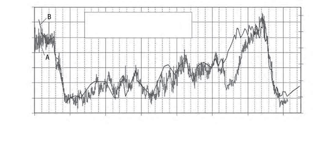
Most paleoclimatologists believe that CO2 lagged temperature during the ice ages because it takes several hundred years for CO2 to come out of, or get into, the world’s oceans, which is where the bulk of the CO2 on our planet is stored.

he oceans can hold much more CO2 (and heat) than the atmosphere. Warm water holds less CO2 than cooler water, so the oceans release CO2 when the temperature goes up, but take it in as the Earth cools down. he lag time is related to what oceanographers call the ocean-mixing time for CO2. 209, 210

Figure 4.1: The CO2 – Temperature Lag

Source: Pangburn.206 Note that time in this chart advances from right to let, with the present on the extreme let of the igure and the distant past on the right.

TABLE 4.3: Co2 SENSITIvITY

The IPCC position

• The major CO 2 feedbacks, which control the climate’s response to added Co2 in the atmosphere, are positive feedbacks that amplify the effect of Co2 on its own.

• The climate sensitivity, which measures any global warming from CO 2, has remained unaltered from the time of the ice ages until now.

• Global warming at the end of ice ages was aided by positive CO 2 feedback, though the feedback lagged the temperature by 600 to 800 years.

• Today’s global warming is also assisted by positive CO 2 feedback, but the feedback switches on almost immediately.

WHAT’S WRONG WITH THIS PICTURE?

1. Recent satellite observations show strongly negative feedback from clouds. If this negative cloud feedback dominates the positive feedbacks from water vapor, and from snow and ice, the net Co2 feedback is negative – diminishing the warming from Co2 to an insigniicant level.

2. IPCC climate models greatly exaggerate climate sensitivity, partly because of assumptions made about atmospheric water vapor, and partly because of faulty statistical analysis.

3. Climate conditions during the ice ages were radically different from today, so it’s unlikely that the climate sensitivity is still the same, as assumed in most computer climate models.

4. Co2 lagged temperature during post ice-age warming due to its delayed release from the oceans. But because of the lag, atmospheric Co2 kept rising for 600 to 800 years after the temperature leveled out. In the modern era since 1850, the Co2 level and temperature have increased together. This two-faced CO2 behavior makes no sense.

A recent study asserts that increased CO2 led, not lagged, global warming at the end of the most recent ice age, based on a variety of proxy data. Jeremy Shakun and his coauthors postulate that while CO2 trailed temperature in the Antarctic when the ice age terminated, as you can see by looking carefully at Figure 4.1, higher CO2 levels preceded warming over the globe as a whole.211 his conjecture is an extension of earlier proposals by other paleoclimatologists,212 on a more rapid timescale.

But a detailed, independent analysis of the same proxy data has found there is so much scatter in the data that whether CO2 leads or lags the warming can’t even be established!213 he study’s claim to the contrary is reminiscent of the hockey stick episode (Chapter 2), when the IPCC tried to latten out the bumps in the historical temperature record to make it conform to the CO2 record, for the purpose of bolstering its hypothesis that global warming is a direct consequence of human activity

It’s not hard to see what the alarmist authors of the CO2 lead study were up to. he CO2 hypothesis requires warming from human CO2 to follow the rising CO2 level, not the other way round. So, just as Mann and his colleagues had already done with temperatures over the past millennium, Shakun and his coauthors have deceptively done with the temperature record as the Earth emerged from the last ice age, to make it look like the gain in CO2 triggered warming.211 hat is, enhanced CO2 causes global warming, whatever the source of the CO2 – then and now.

Nonetheless, the observed CO2 lag does indeed deal a deathblow to the notion of man-made global warming. he reason has to do with the behavior of the temperature and CO2 level just beyond the cessation of an ice age.

Ice ages are believed to have ended (and begun) because of changes in the Earth’s orbit around the sun.214 Ater tens of thousands of years of bitter cold, the temperature suddenly took an upward turn. As we’ve just seen, warmer conditions make CO2 less soluble in water, causing the oceans to give up CO2 to the atmosphere as the temperature increases, a process that takes 600 to 800 years

According to IPCC climate modelers, the melting of ice sheets and glaciers caused by the slight initial warming could not have continued, unless this temperature rise was ampliied by positive feedbacks – including CO2 feedback, triggered by the surge in atmospheric CO2 as it escaped from the oceans.215 Aided

by the feedbacks, says the IPCC, a period of global warming ensued, with the temperature climbing until it reached a new, higher equilibrium level that signaled the end of the ice age. A similar chain of events, based on CO2 and other feedbacks, enhanced global cooling as the temperature dropped at the beginning of the ice age.216

he problem for believers in the CO2 global warming hypothesis is that when the ice age was over, the temperature suddenly stopped increasing and leveled out, but CO2 continued to rise for another 600 or 800 years before plateauing and then decreasing slightly. hat’s well documented in the historical record (Figure 4.1).217

But how can rising CO2 in the atmosphere be the cause of escalating temperatures today, yet not 11,000 years ago – and at previous ice-age terminations – when the mercury stood still as the CO2 level kept ascending? If CO2 from the oceans didn’t make the temperature go up during the 600 years or so immediately ater the Earth’s recovery from an ice age, why should CO2 from human emissions make it go up now (the CO2 lag problem in Table 1.2)?218 Perhaps some of the present rise in the CO2 level is the ocean-delayed response to distant medieval warming.

It makes no sense that CO2 feedback should be dragging the temperature upward in our present climate, and did the same thing as the planet pulled out of past ice ages, but then suddenly turned of for the inal 600 to 800 years

he IPCC, in its 2007 report, implies that this two-sided temperature response to CO2 occurs because temperature and CO2 are going up much faster during current global warming than they did at the end of the last ice age.219 he atmospheric CO2 level is indeed growing a lot more rapidly today, but the assertion that the temperature is increasing 10 times faster than in the past is an exaggeration, as you might expect from the IPCC. he warming we’ve seen since 1850 has in fact been only two to three times faster than post ice-age global warming.220 hat’s not such a big diference.

Other questions also arise. For instance, the IPCC asserts that net CO2 feedback has always been positive, from the ice ages to the present. I’ve already discussed the possibility, based on recent satellite observations of clouds, that the net CO2 feedback in our current climate is negative. How can the IPCC be so sure it wasn’t negative instead of positive going into and out of ice ages?

And how certain is it that CO2 feedback was operating at all in glacial times? Other feedbacks – such as from snow and ice – are believed to have played a role in ice-age temperature swings. Perhaps these other feedbacks could have done the job alone, without any help from CO2, the atmospheric CO2 level moving up or down simply in response to the changing solubility of CO2 in the oceans caused by changing temperatures.

Assuming that there actually was CO2 feedback to amplify temperature rises and falls, why was the temperature descent at the onset of an ice age so much slower than its rapid climb at the end?

If you’re beginning to think there’s more uncertainty than certainty in global warming science, you’re right. he CO2 hypothesis and the whole theory of human-induced global warming, for a theory is what it is, are a limsy house of cards.

Chapter 5: Doing What Comes Naturally

As we’ve seen in the last few chapters, man-made CO2 is highly unlikely to be the main cause of climate change. he whole IPCC case for CO2 warming is shot through with problems, from inconsistencies in the CO2 hypothesis to overconidence in computer models to distortion of data to corruption. he science behind the IPCC’s reports is so badly lawed that it’s hard for me to believe that so many alarmists accept them as an act of faith.

But if it isn’t CO2, what’s heating up the planet?

An honest answer to the question would be that we just don’t know right now. It’s not that we’re short of ideas, but we simply don’t have enough evidence at the moment to draw any irm conclusions – except that the chances of CO2 being the number one culprit are very, very slim.

If humans are not to blame, the obvious place to look for an alternative explanation is nature. It’s well known that natural cycles have altered the Earth’s climate many times in the past, notably the orbital changes that sent the globe into the deep freezes of the ice ages.

Nobody is suggesting that our current warming spell has anything to do with the Earth’s orbital cycles, but there are several other candidates in the natural world. One, or a combination, of these natural cycles could well be responsible for global warming. In this chapter, we’ll examine two of the main contending alternatives, solar variability and ocean oscillations, along with their efect on clouds.

NATURE’S WARMING: THE SUN

It was suspected that the sun is connected to the Earth’s climate soon ater the invention four hundred years ago of the telescope, which made it possible to see sunspots (and other astronomical quirks) more clearly. Sunspots are small dark blotches on the sun’s surface caused by magnetic storms in the solar interior.

During the so-called Maunder Minimum (Figure 5.1), a 70-year period in the 17th and 18th centuries that formed part of the Little Ice Age, there were hardly any sunspots at all. In 1801, British astronomer William Herschel proposed that sunspots were linked to the weather, observing that the price of wheat had been high during that low-sunspot period, which he thought relected poor harvests because of the cooler conditions.

Although Herschel was not able to prove his case at the time, U.S. astronomer John Eddy almost 200 years later established that sunspot variations have been associated with changes in the Earth’s climate for thousands of years. he variation in sunspot number over time is but one of many solar cycles.

Rhythms of the Solar System

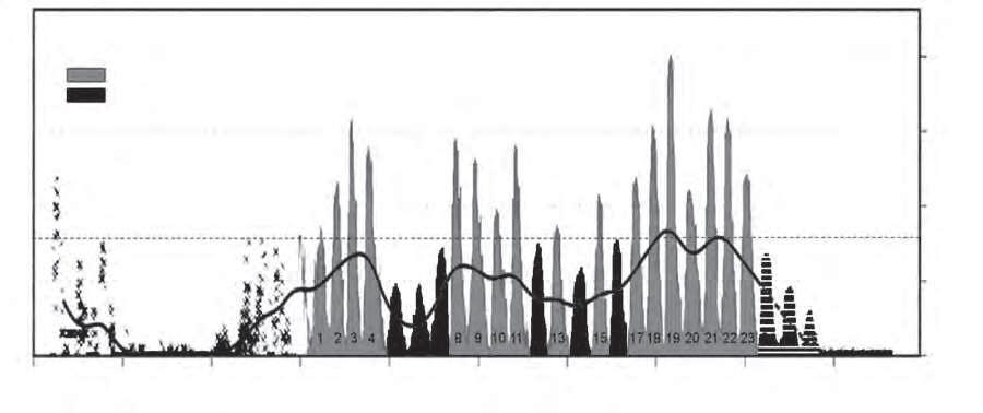
he solar system is constantly pulsating. As we know, all the planets, including our own, orbit the sun and spin on an axis. But the sun is not motionless either: it too rotates on an axis and, because it’s tugged by the gravitational pull of the

Figure 5.1: The Sunspot record from 1611

Source: Abdussamatov.221 he three striated peaks on the right of the igure for solar cycles 24, 25 and 26, and the minimum of 2042, are forecasts.

giant planets Jupiter and Saturn, orbits in a small but complex spiral around the center of the solar system.222

All this pulsation results in a large number of natural cycles tied to the sun, the sunspot count over a year being but one such cycle. he annual sunspot number goes up and down over an interval of about 11 years, and the cycle duration luctuates as well, from as short as 9 years to as long as 14 years.

Along with the number of sunspots, the sun’s heat and light output223 waxes and wanes during the solar cycle. Although this variation in itself is too small, at about one part in a thousand, to have any appreciable efect on our climate, the average value of the sun’s output changes slowly with time – and these changes can cause warming and cooling of the Earth’s surface. he changes in average solar output correspond closely to the pattern shown by sunspot numbers in Figure 5.1.

here are cycles longer than 11 years too. Not only do solar output and the sunspot number repeat every 11 years or so, but their maximum (and minimum) values also make extra big jumps every 87 years and again at 210-year intervals.

he 87-year and 210-year cycles may be associated with a newly discovered climate cycle approximately 1,500 years long, which has manifested itself during both the Earth’s ice ages and warmer interglacial periods, including the one we’re in today. he 1,500-year (plus or minus 500) cycle is described at length elsewhere,224 so I won’t dwell further on it here.

he 87-year solar cycle has been linked to a number of regional climate luctuations, exhibited for instance by temperatures in central England since 1700, rainfall in Beijing and looding of the Nile River in Africa.225 he 87-year cycle has also been used to predict the future occurrence of a protracted cold stretch around 2030, with temperatures comparable to those experienced during the Maunder Minimum period of the Little Ice Age.226 Another prediction links the 210-year solar cycle to an upcoming freeze, in the vicinity of 2040-2050.221

Mathematical physicist Nicola Scafetta has developed an astronomical climate model, in which the changing positions of Jupiter and Saturn in the solar system result in a 60-year climate cycle on Earth.227 As we’ll see later in the chapter, surface temperatures in the Paciic Ocean exhibit a 60-year cycle.

here is also evidence for a 60-year cycle in the rise of global sea levels since 1700 and, says Scafetta, in observed monsoon rainfall cycles as recorded in

ancient Sanskrit texts.228 He believes that a natural 60-year cycle based on Jupiter and Saturn may even explain traditional Chinese, Tamil and Tibetan 60-year cyclical calendars, remarking to a correspondent that “in the Hindu tradition, the 60-year cycle is known as the cycle of Brihaspati, the name of Jupiter”.229

According to the astronomical model, up to 50% of the global warming between 1970 and 2000 may have come from this natural 60-year cycle.227 And much of the other 50% can be attributed to the increase in the sun’s average output since the gloomy days of the Maunder Minimum, Scafetta has claimed in earlier papers.230, 231

However, the exact amount of the solar contribution to global warming is critically dependent on how much the sun’s activity has risen from the time of the sunspot-free Maunder Minimum. Scafetta’s estimate of a solar contribution around 50% hinges on satellite measurements232, 233 that show a post-Maunder Minimum rise in solar output about one third larger than another set of satellite data.234

here has been considerable debate over which satellite data set is the more accurate, especially in establishing the current solar activity level; a recent efort to resolve the diference was controversial.235 Solar physicist Mike Lockwood has argued that the solar activity gain since the Maunder Minimum is more in line with the second, lower set of satellite measurements236 – in which case the solar portion of current global warming is much less than 50%.

But this applies only to direct connections between the sun and the Earth’s climate. As well as any direct solar inluence, indirect solar efects can have an impact on the warming and cooling of our planet. Possible indirect efects include cosmic rays from deep space, the sun’s own ultraviolet (UV) radiation, something called the solar wind,237 and even other natural climate cycles.

Some sort of ampliication mechanism is required, however, for there to be a signiicant contribution to global warming from any of the solar cycles that I’ve discussed here, or from indirect solar efects.

Nevertheless, despite the attempts by the IPCC in its latest report to minimize the sun’s contribution to global warming,238 the need for a solar ampliication mechanism should not be dismissed lightly. Ater all, in the IPCC’s computer climate models, it’s primarily ampliication by water vapor and cloud feedbacks that boosts the tiny temperature increase caused by CO2 acting alone.239

-84-

Potential sources of solar ampliication include any variation in the Earth’s relectivity (albedo),221 which may or may not be associated with changes in cloud cover, water vapor in the atmosphere, and two other mechanisms to be discussed in the next sections.

Ampliication Mechanisms: Cosmic Rays from Outer Space

Fluctuations in the sun’s output are small, about a tenth of one percent over the 11 years of the sunspot cycle, and perhaps only as much or a little more during the 300 years since the Maunder Minimum ended in the early 18th century. But this may be enough to explain a substantial part of our current global warming, even though the IPCC wants us to believe otherwise.

How can such small changes in the sun’s activity afect our climate at all?

One answer is in indirect solar efects – not the direct efect of the sun’s heat, which is absorbed by gases in the atmosphere, by clouds, by the oceans, and by land surfaces;240 but secondary, indirect efects associated with galactic cosmic rays, the sun’s UV rays, or maybe one of the Earth’s atmospheric circulatory patterns. It’s possible that a tiny increase in solar activity could be ampliied by one of these indirect efects.

Cosmic rays are super-energetic, electrically charged particles that come mostly from exploded stars in our Milky Way galaxy and continually bombard the upper atmosphere. But the sun’s solar wind237 can delect these intruders away from the Earth. As the sun becomes more active, the number of cosmic rays hitting the atmosphere falls of; as it quiets down, more cosmic rays get through to the atmosphere.

According to a proposal by Danish physicist Henrik Svensmark, cosmic rays can seed the formation of clouds – especially low-level clouds that cover more than 25% of the Earth’s surface and produce cooling.241

he idea is that a small increase in the sun’s output that decreases the number of cosmic rays can therefore reduce the cooling efect from low clouds, amplifying the direct warming efect from the sun itself through a positive feedback process. In Svensmark’s words, the connection between clouds and cosmic rays provides “a mechanism for solar-driven climate change more powerful than changes in solar irradiance”.242

Svensmark claims that this indirect cloud mechanism can explain not only modern global warming, but also the 1,500-year climate cycle mentioned in the previous section, and even the onset and termination of ice ages in the very distant past. Millions of years ago, the variation of cloudiness induced by cosmic rays had less to do with solar activity, says Svensmark, than with changes in the number of cosmic rays reaching the sun in the irst place, which luctuated as the solar system moved across the spiral arms of our galaxy.243 Other researchers have found that the number of cosmic rays in the sun’s vicinity does indeed vary, over a cycle of about 140 million years.244

It’s already well established that the slight lickering in the sun’s output regulates the number of cosmic rays that reach the atmosphere today. And Svensmark’s comparison of satellite data on clouds with ground-based cosmic ray counts does appear to show a correlation between low cloud cover and galactic cosmic rays, over the last 30 years.245

However, despite the reduction in cosmic ray intensity during the whole 20th century, which would have contributed to global warming according to the Svensmark theory, his far-reaching assertions are still largely speculative at present. Apart from speculation, the only basis for the notion that cosmic rays are related to low cloud cover is laboratory experiments, which may not be a realistic simulation of actual conditions in the Earth’s atmosphere.

Preliminary experiments, conducted at the Danish National Space Center in Copenhagen, reproduced real-life conditions only at sea level.246 In 2011, the irst of a series of bold, large-scale experiments was completed at the European atomsmashing facility (CERN) in Geneva, using a special “cloud chamber” that can simulate all levels of the atmosphere, together with a high-energy particle beam that mimics cosmic rays at higher altitudes.247

Although the latest experiment appears to support the Svensmark hypothesis of a cosmic ray contribution to global warming, the study has raised new questions that require further investigation – which may take several years.

he proposed mechanism for cloud formation involves cosmic rays breaking air molecules apart to form miniscule quantities of airborne droplets, or aerosol particles, that are made up of tiny clusters of sulfuric acid and water vapor. Atmospheric aerosols are thought to be the building blocks for clouds.248

As anticipated, the CERN results show that sulfuric acid and water vapor can rapidly form small aerosol droplets a kilometer or two up in the atmosphere, and that cosmic rays enhance the formation rate by ten times or more. But the surprise was that, in the lowest layer of the atmosphere, additional vapors are needed to nucleate aerosols.249

So the CERN group is planning future experiments to discover what other vapors are involved, whether they are largely natural or of human origin, and how they inluence clouds.250 he group will also study larger aerosol droplets in the chamber, and even hopes to generate artiicial clouds.247

In the meantime, whether the correlation between low cloud cover and cosmic rays really exists is the subject of intense debate. As in many other areas of climate science, good quality observational data on clouds is hard to come by. A problem with satellite observations is that low clouds are sometimes obscured by middlelevel and high clouds251 that respond diferently to cosmic rays. he picture is further complicated by possible changes in cloud height as a result of global warming (Chapter 4), which makes it more diicult to distinguish between low and middle clouds.

he analysis of a group of Finnish climatologists has endorsed Svensmark’s theory that low cloud cover correlates with cosmic ray intensity, even though the correlation is regional rather than global.252 Although the regional correlation is not restricted to any one area, a global connection is disputed by other researchers, including UK physicists Terry Sloan and Sir Arnold Wolfendale, who maintain that less than 23% of the worldwide decrease in low clouds during solar cycle 22 (see Figure 5.1) was due to the sun’s inluence on cosmic rays.253

Sloan’s research group also inds that changes in cloud cover, both low and high, correlate better with variations in the sun’s UV output – a topic to be discussed in the following section – than with cosmic rays254 .

But a recent upsurge in cosmic ray counts around the world may swing the pendulum back toward the Svensmark hypothesis. he intensity of cosmic rays has risen noticeably since the mid-2000s,255 relecting a slight drop in solar activity that is also seen in declining sunspot numbers (Figure 5.1). his fallof in solar activity may foreshadow future global cooling, such as the big freeze predicted from the 87-year and 210-year solar cycles and discussed earlier in the chapter.

he IPCC is hedging its bets on cosmic rays for now, saying that while “empirical associations have been reported between globally averaged low-level cloud cover and cosmic ray luxes”, its level of scientiic understanding of cosmic ray inluences is “very low”.256 his very low understanding has evidently prompted the IPCC to omit all indirect solar efects from its computer models, although its marginally higher “low” understanding of direct solar efects257 hasn’t prevented it from including these in the models.

Ampliication Mechanisms: Ozone

A second indirect heating efect of the sun, possibly more important than cosmic rays, implicates the ozone layer.

You’ve probably heard about the holes in the ozone layer, which are a concern because they allow more of the sun’s harmful UV radiation to penetrate the atmosphere and make it to the Earth’s surface in regions of the globe underneath the holes. he ozone layer, which is located in the upper atmosphere,258 normally protects us from nearly all UV rays by absorbing them. Some ozone also resides in the lower atmosphere.154

As the sun’s output of heat and visible light luctuates, so too does its production of invisible UV, which varies much more over the 11-year solar cycle than the tenth of a percent change in total solar output.259 A more active sun generates more UV radiation, which creates more ozone in the ozone layer 260 he slightly thicker ozone layer provides a little extra UV protection for humans by absorbing more sunlight.

Absorption of solar UV also warms the ozone layer, since all forms of radiation from the sun (including visible light, UV and infrared) carry heat energy. his in turn heats both the upper and lower atmosphere261 and ampliies the direct warming caused by solar activity – a positive feedback process.

he ampliication associated with positive feedback can also magnify cooling efects when the sun’s UV output declines. A second positive feedback connected with variations in solar activity involves shits in atmospheric wind patterns produced by UV changes.262 Lockwood has proposed that the wind shits may be related to very cold European winters since about 2009 – perturbations of upper atmosphere winds by lower UV levels resulting in “blocking” of the north polar

jet stream,263 a high-altitude air current that governs much of the weather in Europe and North America.

Meteorologists think a lazy jet stream caused by a downturn in UV from a quieter sun may explain many of the prolonged heating and cooling spells that have become prevalent in the Northern Hemisphere recently.264 Blocking produces unusual holding patterns that can keep a weather system in one place for extended periods.

And there may even be a link between solar UV and cloud cover – a link that can contribute indirectly to global warming, as we’ve just seen with cosmic rays. Two of the studies mentioned in the previous section, which found a correlation between cosmic ray strength and low cloud cover, also noted a correlation of solar UV output with middle cloud cover.252, 254 Middle level clouds can either cool like low clouds, or warm like high clouds.

However, the exact amount of indirect warming produced by solar UV acting on the ozone layer is unknown at present. Atmospheric physics researcher Joanna Haigh in 2003 cited several studies, all of which suggest that climate models “may underestimate solar inluence by up to a factor of three” because the models omit ozone heating efects.265 But in a later paper, Haigh says her research team’s analysis of recent UV measurements suggests that the sun’s indirect contribution to global warming may in fact have been overestimated.266

Other Planets

If the sun is playing a role in global warming on Earth, we would expect the other planets in our solar system to show signs of warming as well. Planetary global warming may indeed exist, but the evidence is rather thin at the moment and there is an extreme scarcity of both data and scientiic studies.

Even with the annual publication of thousands of research papers on the climate of our own planet, there’s plenty of disagreement about what is causing temperatures to rise – despite the constant eforts of the IPCC and climate change alarmists to convince us that CO2 is the villain. So we shouldn’t pay too much attention to what are just a handful of articles on warming trends elsewhere in the solar system.

An example of how easy it is to be misled by limited data can be found in recent studies of Mars, where dust storms are prevalent.

From darkening of the planet’s surface, a team of space scientists calculated that in the 22 years between two NASA missions to Mars, it had warmed by 0.65o Celsius (1.2o Fahrenheit). his is almost as much global warming as we’ve experienced here on Earth in 160 years. Attributing the apparent warming to changes in sunlight-relecting surface dust, though not to solar activity, the research team linked the sudden temperature rise to melting of the ice cap near the Martian South Pole over the past few years.267

But a diferent group of investigators pointed out that the irst mission to Mars had come right ater a global dust storm there that had made the planet appear much brighter than it looked 22 years later, and concluded that surface brightness doesn’t tell us much about Martian warming.268 he melting of the southern ice cap could also have been associated with changes in dust coverage and, in the absence of other data, doesn’t make a strong case for global warming on Mars.

Another reason to be skeptical about evidence for global warming on other planets is that most planets have very long “years”.

It takes 165 Earth years for Neptune to orbit the sun once, for example, which means we need to wait a long time to ensure that any warming trend we notice isn’t just from the changing Neptunian seasons. Possible global warming reported on Neptune,269, 270 on Neptune’s moon Triton,271 and on Pluto272 have all been ascribed, at least partly, to planetary seasonal efects.

One planet where CO2 has unquestionably caused global warming is Venus, which has a dense atmosphere consisting of 97% CO2, far above the Earth’s current CO2 level of 393 parts per million (0.039%). he runaway greenhouse efect on Venus produces furnace-like conditions, with a surface temperature around 470o Celsius (880o Fahrenheit). But that’s how it’s been there for billions of years and the planet isn’t currently getting any warmer from the sun.

More IPCC Shenanigans: Solar Warming Minimized

he IPCC has done it again.

As we saw in earlier chapters, the IPCC and its supporters have indulged incessantly in exaggeration, data tampering and deception to bolster their case for man-made climate change.

he same wiliness can be found in the IPCC’s treatment of historical data for solar activity, where the goal was to make the contribution of solar variability

to global warming appear lower than it may actually be. he sun’s luctuations probably can’t explain all the global warming to date, but the IPCC’s Fourth Assessment Report in 2007 minimizes the solar contribution almost to the point of insigniicance by cherry-picking the historical record.

Proxy records of solar intensity include both sunspot numbers and so-called cosmogenic isotopes, which are trace amounts of radioactivity let in proxies such as ice cores and tree rings by past cosmic rays from space. As the sun’s output varies, the radioactivity levels of these isotopes rise and fall, leaving an imprint of solar activity at the time.273

he variation in solar activity includes short-term luctuations during the sun’s 11-year cycle, as well as longer-term increases or decreases in the average solar output that can have a signiicant efect on climate. As we saw earlier in the chapter, how much the sun is contributing to global warming depends on how much the sun’s average energy has risen since the Maunder Minimum, the period from 1645 to 1715 when there were almost no sunspots and solar activity was low – the years that coincided with the chilliest episode of the Little Ice Age.

According to the IPCC,274 the sun’s output right now has increased only slightly over the 300 years since then. If the IPCC is correct, it means that any solar contribution to global warming today is minimal. However, the IPCC’s conclusion about the sun’s output is based on a very selective choice of historical data, namely the plucking out of one of the lowest available estimates of the boost in solar output since the Maunder Minimum.

he problem is that actual measurements of solar activity, apart from sunspot counts, date only from the beginning of the satellite era in 1978. To ill in the rest of the gap between the Maunder Minimum and now, we have to rely on theoretical reconstructions of solar output, based on a variety of proxies. Consequently, as stated in a recent review of the sun-climate connection, “…the extent of the positive drit in TSI [solar activity] between the Maunder Minimum and the present day is uncertain”.262

he IPCC’s low estimate of the increase in solar activity during the last 300 years is derived from a reconstruction based on recorded sunspot numbers and a computer model.275 While computer simulations of the sun are probably no more reliable than computer climate models, other reconstructions of solar activity using diferent methods have arrived at similar low estimates.

he 2007 IPCC report actually lists several estimates of the solar activity gain since the Maunder Minimum, the selected high estimate being three times larger than the low one based on sunspot proxies,276 but calculated instead from ice-core radioactivity levels.277

Needless to say, the IPCC then goes on to ignore all but the lowest estimate to calculate the solar contribution to global warming.278 Obviously, a bigger increase in the sun’s average output since the end of the 1600s would account for more of our recent global warming than the IPCC wants to admit.

In its 2001 hird Assessment Report, the incorrigible IPCC resorted to a diferent subterfuge to minimize the sun’s efect on global warming.

Most of the estimates in that report weren’t based on proxy data from sunspots or ice cores, but on comparisons between the sun and similar stars, a method that is now largely discredited. But these comparisons yielded calculations of the solar activity gain since the Maunder Minimum even larger than the high estimate that the IPCC rejected for its 2007 report. To lower the big diference in solar output between past and present, the IPCC deviously measured the present-day increase only from the year 1750279 – well ater the Maunder Minimum was over, and the sun’s intensity and the number of sunspots had returned to more normal levels. his ruse cut the solar activity increase since 1700 in half.

Once more, and on two separate occasions, the IPCC has cast aside the rules of science to prop up its unconvincing case for man-made CO2 as the source of global warming. As I discussed earlier, one of the cornerstones of the scientiic method is that you don’t ignore or discard data just because it doesn’t it your theory. Properly conducted science examines all the data, without bias.

So determined has the IPCC been to trivialize the role played by the sun in climate change that it doesn’t even bother to enumerate the solar contribution in its 2007 report. It appears that the IPCC estimates the solar portion of total global warming at only a few percent.280

But there’s plenty of evidence that solar activity has increased considerably over the last 300 years, and that the sun’s role in global warming has been underrated in IPCC computer climate models.

NATURE’S WARMING: THE OCEANS

Natural climate variability includes several patterns of cyclic behavior. hese come about through changes in wind and ocean circulation over months or years, but reveal themselves as luctuations in temperature, rainfall and other features of our daily and weekly weather

he familiar El Niño and La Niña cycles arise from seesaw changes in tropical ocean surface temperatures that cause drastic shits in climate around the Paciic Ocean,281 for periods of a year or more at a time. he 1997-1998 El Niño, one of the strongest on record, raised surface temperatures around the world by 0.17o Celsius (0.3o Fahrenheit)282 – which is an appreciable fraction of the total global warming since 1850 – for a full year. More serious efects of El Niño and La Niña can range from catastrophic looding in the U.S. and Peru to severe droughts in Australia. he cycles recur on a regular basis, although the intervals between them can vary quite a bit.

Other ocean oscillations that repeat at intervals from years to decades include the Paciic Decadal Oscillation, the North Atlantic Oscillation, the Arctic Oscillation and the Atlantic Multidecadal Oscillation. Although IPCC computer climate models endeavor to simulate the various cycles, the models have been unsuccessful at predicting the timing and climatic efects of several of them.283

Before we look at one of these cycles (the Paciic Decadal Oscillation) in more detail, we’ll pause to examine several examples of a new line of investigation in climate science, involving interconnections between ocean oscillations and solar variability. It’s becoming increasingly apparent that the sun, the oceans and even clouds are tied together, as well as to the atmosphere, and it’s quite possible that their interactions have a far bigger efect on climate than CO2.

he Sun-Ocean Connection

In studying the 1,500-year solar cycle discussed at the beginning of this chapter, geologist Gerard Bond and his colleagues suggested two ampliication, or positive feedback, mechanisms through which very small drops in solar activity may have triggered substantial climate change many times over the last 9,000 years.284 he changes include abrupt cooling in the Netherlands, glacial advances in Scandinavia and markedly reduced rainfall in the Persian Gulf.

One of the suggested ampliication mechanisms involves changes in the ozone layer, which I’ve already discussed. he other involves the oceans.

he hypothesis is that a slight fall in solar output could have slowed the turning over of deep ocean currents in the North Atlantic by lowering surface salinity. A similar slowing occurred at the end of the last ice age, caused not by the sun but by the sudden melting of ice sheets.285 he overturning of ocean water is part of the ocean conveyor belt that circulates water and heat around the globe, so any phenomenon such as solar variability that alters this circulation can afect global temperatures. In this case, the slowdown of the conveyor belt would have intensiied the initial solar cooling, but the slowing could have been triggered equally well by solar warming.

A rather diferent ocean ampliication mechanism has been proposed by a group of climatologists, in trying to explain the pronounced response of the Paciic Ocean climate system to the small variation in solar activity over the 11-year sunspot cycle.286

he explanation involves another “bottom-up” mechanism, in which the additional ocean heating caused by a slightly stronger sun results in increased evaporation. his in turn produces heavier rainfall, stronger winds and fewer low clouds in the Paciic – raising sea surface temperatures, since low clouds cool, and amplifying the original warming via positive feedback. A similar explanation applies to cooling. he combined efect of this bottom-up mechanism with “top-down” ozone ampliication is to magnify direct solar heating by four times or more.287

Since oceans can store and transport vast amounts of heat – a characteristic known as thermal inertia – there is a time lag between changes in solar activity and corresponding changes in temperature. he oceans absorb most of the sun’s incoming heat near the equator and then transport it north or south, a process that takes about 8 to 12 years.226, 288

Because this time lag is approximately as long as an 11-year solar cycle, global surface temperatures in any particular cycle are determined by the length of the previous solar cycle, a recent Norwegian study has found – at least in the North Atlantic. he study also found that the solar contribution to global warming over the last 150 years was about 40% in Norway and up to 70% in nearby locations such as Iceland.289

And, from an analysis of luctuations in ocean heat content, a topic I’ll return to in the next chapter, Israeli physicist Nir Shaviv has concluded that total solar forcing is from ive to seven times larger than that associated with direct solar warming. Such a large ampliication factor would imply that the Earth’s climate is much more sensitive to the sun than to CO2 290 Of the various possible indirect ampliication mechanisms, Shaviv favors cosmic rays.

he Paciic Decadal Oscillation (PDO)

he Paciic Decadal Oscillation (PDO) has characteristics in common with El Niño and La Niña, but the cycle time is much longer – about 60 years for a full PDO cycle, compared with two to seven years between successive El Niño or La Niña events. Although the luctuations of the PDO can be traced back at least several centuries, its distinctive pattern wasn’t recognized until the 1990s, when it was named by a U.S. isheries scientist trying to explain the connection between Alaskan salmon harvests and the Paciic climate.

he PDO cycle switches between warm and cool phases. During the 30-year warm phase, when more El Niños occur, ocean surface temperatures in the northeastern Paciic are higher than normal, and the southeastern U.S. is cooler and wetter than usual. he 30-year cool phase, marked by an excess of La Niñas, is dominated by correspondingly lower ocean temperatures and warmer, drier conditions inland.

he other major multidecadal ocean cycle is the Atlantic Multidecadal Oscillation (AMO), which has a cycle time of approximately 65 years. Like the slightly shorter PDO, the AMO alternates between warm and cool phases, although the warm phases usually last longer. he two cycles are compared in Figure 5.2.

Because the cycle times for the PDO and AMO are close to 60 years, it’s possible that one or both of these ocean oscillations is related to the proposed 60-year solar cycle underpinned by the motions of Jupiter and Saturn,227 a theory discussed earlier in the chapter. However, the astronomical model on which this theory depends is just a model and, like computer climate models, contains arbitrary adjustable parameters – though fewer of them.

Meteorologist Joe D’Aleo and others have pointed out that the warm and cool phases of the PDO coincided with the major periods of warming and cooling, respectively, in the 20th century.291 Even though the overall trend in tempera-

GLOBAL WARMING FALSE ALARM

tures since 1850 has been upward, there have been at least two intervals when the mercury took a dive for a decade or more (Figure 1.1). Each time that the PDO mode shited from warm to cool, or vice versa, global temperatures switched accordingly.

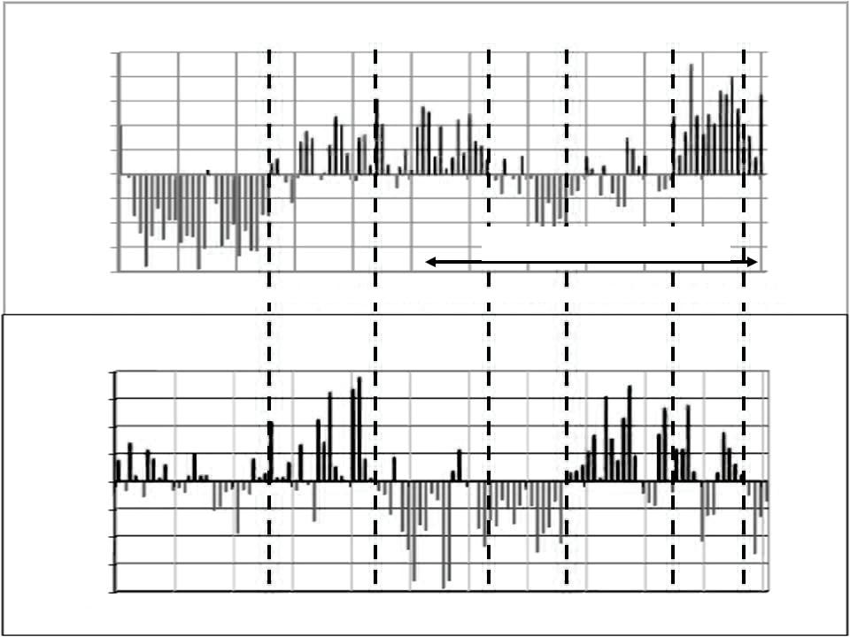
To some skeptics, this coincidence explains global warming. But while the PDO may be an explanation for global warming, it is not simply because the temperature follows the warm and cool phases of the oscillatory cycle.

Roy Spencer and his research team at the University of Alabama in Huntsville have hypothesized that cloud changes associated with the PDO may be able to account for much of measured global warming,292 which the IPCC and climate change alarmists insist on attributing to CO2. he University of Alabama group is the same one that found evidence in satellite observations for negative CO2 feedback from clouds, a subject discussed in Chapter 4. he new global warming hypothesis also relies on satellite data.

Figure 5.2: The AMO and PDO since 1900

Most like the 1940s-1960s

Source: ICECAP.293 he vertical scale shows the AMO or PDO index – a measure of Atlantic or Paciic surface temperature, respectively. A positive index indicates warming, a negative index cooling.

TABLE 5.1: NATURAL WARmING – ALTERNATIvES To Co2

Alternative

1. Solar variability

• Solar 11-year, 87-year, 210-year and possibly 60-year cycles.

• An increase in the sun’s average output over the 300 years or so since the maunder sunspot minimum during the Little Ice Age.

• Indirect ampliication from the sun’s delection of cosmic rays. Thi s delection may reduce the cooling from low clouds when the sun is more active.

• Indirect ampliication from the sun’s UV radiation, which warms the ozone layer and shifts wind patterns in the upper atmosphere, and may affect clouds in the lower atmosphere.

2. Sun-ocean connections

• Ampliication from the interaction of the sun and oceans, via the slowdown of deep ocean currents caused by reduced surface salinity.

• Ampliication from the interaction of the sun and oceans, via a reduction in low cloud formation resulting from heavier rainfall.

3. Cloud luctuations associated with the Paciic Decadal Oscillation (PDO), a natural climate cycle that switches between warm and cool every 30 years.

WHAT’S WRONG WITH THIS PICTURE?

• The IPCC claims erroneously that nearly all global warming is caused by manmade Co2, and that natural climate variability plays almost no role.

• The IPCC wrongly assumes that the only natural contribution to the modern warming trend is direct solar effects, and deceptively minim izes even this contribution.

• Potential sources of global warming, such as indirect solar effects, sun-ocean linkages and natural climate cycles like the PDo, are omitted from the IPCC’s computer climate models. most of the models don’t allow for time lags caused by ocean thermal inertia.

• Most of the IPCC’s efforts go into shoring up its case for the f aulty CO 2 hypothesis. very little attention is paid to investigating alternative explanations for climate change – and only minimal funding is available for studying natural variability.

What Spencer postulates is that the natural variability of the PDO causes changes not only in temperature and precipitation, but also in cloud cover. As you may recall, low-level clouds cool the Earth’s surface, while high-level clouds have a heating efect. Warming can originate from either a reduction in low clouds, or an increase in high clouds, or both.

he IPCC, Spencer points out, assumes that this kind of natural cloud variability does not exist and that “the Earth stays in a perpetual state of radiative balance that has only been recently disrupted by mankind’s greenhouse gas emissions”.292 Disputing this IPCC claim, Spencer says that his group has already shown theoretically that random variations in cloudiness on a daily basis can cause ocean temperatures to vary over decades, which is one of the signatures of the PDO.294

he University of Alabama proposal extends this idea to variations in cloud cover that occur not daily, but over timespans of up to 100 years – which might then cause long-term temperature changes such as global warming. Although the PDO is localized in the Paciic Ocean, the mixing of ocean waters around the world over a period of time can result in global cloud luctuations.

Using a simple climate model with very few assumptions, and with luctuations in cloud cover directly related to the observed PDO undulations, Spencer simulated global temperatures for the 20th century.295 Astonishingly, this simple PDO model, on its own, can explain up to 75% of the global warming observed for the whole period from 1900 to 2007.

Analysis of the satellite evidence for PDO cloud luctuations shows strongly negative cloud feedback, just as found in the earlier studies of other cloud data by Spencer’s team.296 Negative feedback diminishes the warming caused by atmospheric CO2 acting alone, to a low or even an insigniicant level.

In 2008, the 30-year PDO warm phase that began in 1977 came to an end (Figure 5.2). his ushered in a new cool phase, just as the shit that occurred in the 1940s resulted in global cooling for the 30 years that followed. It’s important to note that these cooling spells are also predicted by the PDO cloud luctuation model, the basic idea being that the PDO causes long-term variability in cloud cover that leads to global warming and cooling.

Of course, a single study doesn’t make a compelling case for PDO cloud luctuations causing 75% or more of the global warming that we’ve seen so far. But, since the IPCC and climate change alarmists are most likely wrong about CO2,

the PDO theory is certainly a good candidate for an alternative, natural explanation. Further investigation may well validate this alternative theory.

How very diferent these natural explanations are from the CO2 story pushed by the IPCC and climate change alarmists! According to the CO2 hypothesis that we’ve examined at length in previous chapters, nearly all the warming measured since 1850 has been caused by human emissions of CO2.

Natural cycles, such as solar cycles, ocean oscillations and the PDO cloud changes discussed here, have been summarily dismissed by the IPCC – which makes the sweeping assumption that the only source of natural climate variability that contributes to global warming is solar activity 297 And it resorts to deception to minimize even this contribution.

Admittedly, our current understanding of natural variability is poor. But that’s no reason to exclude natural causes, other than the sun, from computer climate models.

he IPCC says its computer models are unable to match the measured temperature record for the 20th century if the models include only natural sources of warming.298 hat’s because the only natural sources simulated by the models are direct solar efects, not to mention the intrinsic limitations of the models themselves. All other natural possibilities, including indirect solar efects such as cosmic rays and ozone, plus sun-ocean connections and climate cycles like the PDO, are omitted.

he IPCC makes much of its supposed ability to detect an “anthropogenic signal” in climate data, especially the temperature record, as substantiation of man-made global warming.299

All this means in reality is that computer climate models, with all their assumptions about CO2 and the climate system, can be adjusted to simulate the climatic record – and that’s not at all surprising, with so many variable parameters to play with. he apparently good it to climate data doesn’t validate the models nor authenticate the connection between CO2 and global warming.

he unlikelihood that CO2 plays any signiicant role in climate change is clear from the temperature record for the 11,000 years that have elapsed since the end of the last ice age.

GLOBAL WARMING FALSE ALARM

During this long interglacial epoch, when human civilization developed and thrived, there have been several periods of global warmth, all of which were warmer on average than our present climate and occurred long before factories and SUVs began adding CO2 to the atmosphere. hese hot spells included the Medieval Warm Period, the Roman Warming about 1,000 years earlier and the Minoan Warming 1,000 years before that (Figure 5.3), along with others.

Source: Foresight Institute.300 he horizontal scale shows the year and the vertical scale gives the surface ice temperature in oC. he Medieval Warm Period corresponds to the peak on the right, the Roman Warming to the two peaks immediately to the let, and the Minoan Warming to the highest peak.

But unfortunately, an adequate understanding of natural climate variations is sadly lacking. For the last 25 years, the climate science community in general, and the IPCC in particular, has been obsessed with CO2. If just a small fraction of the countless hours and weeks of efort that have been wasted trying to justify the CO2 theory had instead been devoted to studying natural causes of rising temperatures, we might by now have had enough data to properly evaluate the alternative explanations.

Figure 5.3: 5,000 Years of Central Greenland Temperatures

Chapter 6: Global Cooling

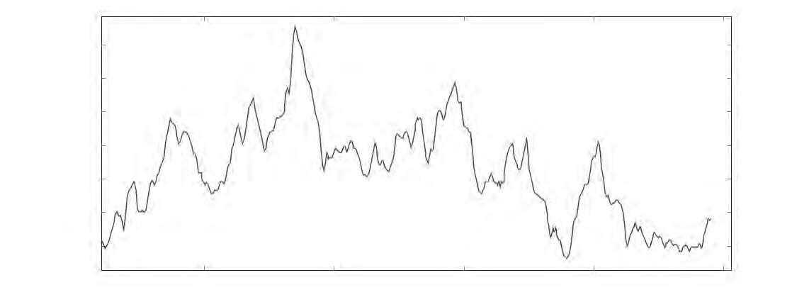
Alternative explanations aside, climate change alarmists now have to grapple with a big nail in the man-made global warming coin. To their enormous embarrassment, global temperatures have been falling – slightly – since about 2001. And this despite the fact that humans are continuing to release more and more CO2 into the atmosphere.

hat’s right, it’s been cooling. As the data comes primarily from NOAA and the UK’s HadCRU, both of which manipulate temperatures to exaggerate global warming as we saw in Chapter 2, you can be pretty sure that the modest amount of cooling these two temperature custodians admit has occurred is really an underestimate – and that the actual drop since 2001 is much bigger than they’re saying.

Perplexed, global warming alarmists around the world are calling the cooling a “hiatus”. But by 2012, the hiatus was at least 11 years old and counting.301 If it persists for another few years, the argument that periods of less than 10 to 15 years are too short to deine a climate trend will lose its validity, and a lot of climatologists will have egg on their face.

REVERSAL OF FORTUNE

Despite warmist protestations about the veracity of reports on the cooling trend when it irst became evident several years ago, the temperature downturn gained credibility in 2009 with the release of a study by two mathematical scientists at the University of Wisconsin-Milwaukee.302

GLOBAL WARMING FALSE ALARM

hestudyfoundnotonlythatglobaltemperatureshaveleveledofanddecreased since late 2001, ater rising steadily for the previous 30 years (see Figure 6.2), but also predicted that the cooling will continue for several decades. Stating that the cool spell can’t be attributed to any particular cause, although it must be natural, coauthor Kyle Swanson remarked, “his is nothing like anything we’ve seen since 1950”.303

Figure 6.1 displays average global temperatures since 2001, showing the unmistakable dip. Up to 2011, the worldwide average temperature had declined about 0.05o Celsius (0.09o Fahrenheit) from 2001.304 he decline cancels out about 10% of the gain from the warming spurt between 1970 and 2000.

Source: RSS 306 he connected data points, from the RSS satellite record, show the temperature anomaly in oC at monthly intervals since 2001, while the sloping line is a trend line.

You’ll be wondering, no doubt, how the IPCC and climate alarmists are dealing with all this. It certainly came as a shock to the global warming faithful, as a frustrated Kevin Trenberth’s Climategate email in 2009 reveals:

Figure 6.1: The Recent Temperature Record

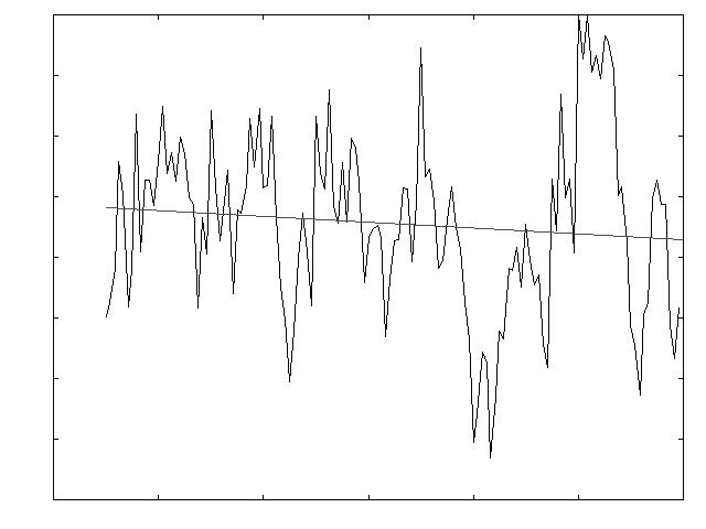
Well … where the heck is global warming? … he fact is that we can’t account for the lack of warming at the moment and it is a travesty that we can’t. he … data are surely wrong. Our observing system is inadequate.305

If experimental observations don’t match the theory, blame the data or the measurements!307 We’ll see another example of this contorted thinking later in the chapter.

Some alarmists at the time declared that cooling was really part of global warming.308 But once the folly of such illogical and farfetched reasoning was exposed, the alarmists adopted a more desperate ploy – that the new signature of CO2-induced climate change should be extreme weather events, not higher temperatures. However, the general public isn’t buying this idea.

Nonetheless, we should recognize that an extended period of cooling – even if it lasts for another 30 years – isn’t necessarily the end of global warming. Shown below (Figure 6.2), and also in Chapter 1, is the temperature record from 1850, which is roughly when modern global warming is considered to have begun. As you can see, there have been several cooling stretches over this time, during which the mercury climbed about 0.8o Celsius (1.4o Fahrenheit) overall.

he chart in Figure 6.2 can be divided into ive time periods of close to 30 years

Figure 6.2: The Temperature Record from 1850

Source: HadCRU. 309

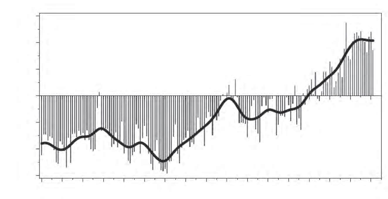
each, in which the temperature alternately rose and fell. From 1850 to 1880 the temperature increased; from 1880 to 1910 it went down again, only to go up once more until 1940; and so on.

Computer climate modelers attribute the cooling that occurred between 1940 and 1970 to aerosol particles in the atmosphere, generated by coal-ired power plants that mushroomed during the period of accelerated industrial development ater World War II. According to believers in the CO2 hypothesis, this cooling efect dominated the warming trend from CO2 emissions for all those years, but gave way to overall warming in the 1970s as clean air acts in several countries reduced global emissions of sulphate aerosols.310

Convenient as this explanation may be, nevertheless, it doesn’t readily account for the current cooling trend. Present global aerosol emissions are thought to be well below those of the post-World War II period, despite the rapid industrialization of China and India, where aerosol emissions are rising. And even the alarmist IPCC concedes that its level of scientiic understanding of aerosol forcing ranges from “low” to “medium-low”.311

he temperature decline from 1940 to 1970 could equally well be associated with luctuations in natural cycles, something that computer models ignore. In fact, the alternating pattern in the temperature record shown in Figure 6.2 goes back all the way to 1470, with a cycle time of around 27 years.312

hat 30 years is the cycle time for the warm or cool phase of the Paciic Decadal Oscillation and also approximately for the Atlantic Multidecadal Oscillation may be signiicant, though our knowledge of both natural cycles is too limited at present to draw any deinite conclusions from this observation. here may also be a connection to the proposed 60-year solar cycle that I discussed in Chapter 5, the cycle being based on an astronomical model that correctly reproduces the current cooling trend.

What will happen when the recent dip in temperature comes to an end is anyone’s guess. Based on the 30-year historical pattern just discussed, we might expect another bout of warming. Indeed, the University of Wisconsin study concludes that the present cooling is “superimposed upon an overall warming presumably due to increasing greenhouse gases”.302

But this assumes that the underlying climate driver is CO2, an assumption that is very likely incorrect as we’ve seen. And even though the study authors profess

-104-

allegiance to the CO2 hypothesis, that may be just for the purpose of maintaining their standing in the climate science community.

As discussed in Chapter 4, the sensitivity of the Earth’s climate system to added CO2 is unlikely to be anywhere near as high as the IPCC claims. he very fact that we’re currently in a cooling period while CO2 is still rising attests to low CO2 sensitivity.

So it’s not at all certain that temperatures will resume their previous ascent when the natural source responsible for the present decline switches of in perhaps 20 or 30 years. It’s entirely possible that some other source of natural variability will kick in and keep the temperature trending down.

We saw in the previous chapter how the sun’s 87-year and 210-year cycles may result in much cooler conditions by 2030 or 2040. In addition, an irregular solar cycle resulting from magnetic changes inside the sun is likely to send it into what is known as a grand solar minimum, within the next 40 years.313, 314 And according to the Norwegian study cited in Chapter 5, the 13-year extent of solar cycle 23 (see Figure 5.1) – almost two years longer than normal – already portends a drop in temperature of at least 1.0o Celsius (1.8o Fahrenheit) in Norway and the North Atlantic, during cycle 24 that ends around 2020.288 hat’s more than the global warming increase for the Northern Hemisphere over the last 160 years!

By analogy to the pattern shown by past warmings (Figure 5.3), astrophysicist Gordon Fulks has suggested that the present bout of cooling may signify a turning point in the modern warming trend, which really began shortly ater 1900 (Figure 6.2). Most of the previous interglacial warmings lasted about 200 years, so that the 20th-century upswing should be followed by a 21st-century downswing, each approximately 100 years in length.315 If that’s the case, the temperature may already be on its way down permanently.

But we just don’t have enough knowledge of the climate to make a reliable prediction one way or the other, to say whether it will warm, or cool further, when the present cooling is over. A quick glance at the long-term historical record (Figure 2.3 or Figure 5.3), however, tells us that global temperatures are always going up and down over short periods of time.

CRYING WOLF

Global cooling, even for a limited period, isn’t in the IPCC playbook. If not hell on earth, something close to it is projected by the IPCC’s most recent report, with global temperatures escalating from now until the end of the 21st century and beyond. Along with the nonstop warming, says the report, will come intensiied heat waves, surging sea levels, and prolonged droughts.316

All these projections are based on the IPCC’s computer climate models – which, as we know, rely heavily on CO2 (and other greenhouse gases), with a very small contribution from the sun but not from any other natural sources. he predictions encompass a range of futuristic scenarios that embrace varying estimates of CO2 emissions, global population and economic growth.317

While the various scenarios result in diferent predictions of the assumed temperature leap by century’s end, the warming calculated for the irst few decades until 2030 is almost the same in all pictures. From 2001 to 2011, the global warming projected by the IPCC was about 0.22o Celsius (0.40o Fahrenheit).318

How wrong can one be?

Over these 10 years, average surface temperatures dropped by about 0.05o Celsius (0.09o Fahrenheit), as we’ve seen. his means the IPCC overestimated the temperature for 2011 by close to 0.3o Celsius (0.5o Fahrenheit).319 hat’s about half of the temperature increase since 1970,320 and around one third of that for the whole period since 1850.

Consumed by recent high temperature readings that were the highest in hundreds of years, the IPCC failed to even notice the cooling downturn. Its 2007 report includes recorded temperature data to as recently as 2005, four years into the slump, and yet its projection graphs show the temperature inching up every year from 2000.318 Talk about not having your act together.

he IPCC’s temperature estimates for the irst decade of the century are so far from reality that it’s impossible to give any credence at all to its inlated projections for 2100, projections in which the IPCC claims to have a conidence level of 66%.321

And it’s not just temperature predictions on which the IPCC and alarmists in general are crying wolf. he list of highly questionable IPCC projections for our future climate includes heavier rainfall, more intense hurricanes and widespread thawing of permafrost.322 here’s little likelihood that any of these will occur if

-106-

the climate is dominated not by CO2 emissions, but by natural variability that is currently cooling the globe down.

Global warming alarmists made hay of Hurricane Katrina, the deadly hurricane that struck the U.S. Gulf Coast in 2005, causing widespread looding and devastation. It was all too easy to attribute such a costly disaster to climate change Indeed, the IPCC maintains that “intense tropical cyclone activity has increased since about 1970”, and that tropical cyclones (which include hurricanes and typhoons) are now much stronger and longer lasting than before, due to global warming.323 he IPCC also predicted that future tropical cyclones will become more powerful yet, though the total number is not expected to increase.324

But in fact, hurricanes and tropical storms are currently becoming less intense, if anything. A commonly used measure of tropical cyclone strength and duration is now at its lowest point since the mid-1970s (Figure 6.3). his almost certainly relects recent global cooling, just as the previous upward trend in cyclone activity noted by the IPCC, and visible in Figure 6.3, was indicative of the warming surge that ended in 2000.

Moreover, attempts to link a 2011 spurt in killer U.S. tornadoes to climate change have recently been debunked, by none other than the National Climatic Data Center (NCDC), which is an arm of NOAA. An NCDC analysis shows

Figure 6.3: Tropical Cyclone Activity since 1972

Source: Maue.325

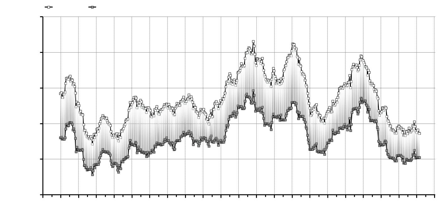
essentially no trend in the incidence of the strongest twisters over the past 55 years.326

A possibly more pressing issue, oten in the news these days, is the extent of Arctic sea ice. For years, those who adhere to the theory that CO2 causes global warming have been lamenting the retreat of glaciers, the disappearance of snow caps from loty mountains, and the shrinkage – from the early 1970s to about 2006 – of the ice cap at the North Pole. If only we’d stop loading the atmosphere with more CO2, they contend, all of this could be reversed.

he shrinking of the polar ice cap has in truth been quite dramatic. Satellite measurements show that Arctic ice cover in the summer months, when the ice is at its minimum extent, contracted at a rate of 7.4% per decade from 1979 to 2005, which is a total reduction of 20% over that period.327

You don’t have to be a rocket scientist (or even a climate scientist) to igure out that, if the same trend continued, the ice cap wouldn’t be here much longer. In 2008, an ice scientist declared that Arctic ice was “in a death spiral” and could be completely gone in summer by about 2030.328 No more ice to fend of the global warming rays of the sun’s summer heat,329 no more habitat for polar bears.

But a funny thing happened on the way to disaster. Since at least 2007, and perhaps a year or two earlier, Arctic ice has been expanding again.330

he summer ice cap in 2008 was 9% larger than the minimum reached in 2007, the minimum that had sent alarmists into such a frenzy. In other words, the gain in just one year was greater than the loss over a whole decade during the 1980s and 1990s. Although summer ice cover in 2011 was only slightly greater than the 2007 minimum,331 winter ice early in 2012 was well above its extent for the last few years,332 especially in the Bering Sea.

Of course, the recovery of the ice cap that appears to be underway is probably linked to the cooling trend discussed in the previous section. Climate change alarmists want none of it, however, and insist that the recovery of Arctic ice is merely part of the global warming hiatus mentioned earlier in the chapter. But we’ve already seen that Antarctic sea ice has been growing for over 30 years, with the result that global sea ice area has remained much the same over the whole period333 – a period during which temperatures rose considerably.

Global cooling, it seems, is here to stay for a while. It will be interesting to see what distortions of the truth the IPCC comes up with in its next assessment

GLoBALCooLING TABLE 6.1: GLoBAL CooLING

The IPCC’s stand

• Global temperatures will continue to increase steadily through the end of t he 21st century, unless we rein in our emissions of Co2.

• Consequences of global warming such as more intense hurricanes, shrinkin g of the Arctic ice cap, and retreating glaciers, will get worse without action on Co2

• Missing heat from the ever increasing CO 2 level must be hiding in the deep ocean, a conclusion reached since publication of the IPCC’s 2007 report.

• The oceans will continue to warm overall, causing sea levels worldwide to rise drastically.

WHAT’S WRONG WITH THIS PICTURE?

1. man-made Co2 is highly unlikely to be the primary cause of global warming, as discussed in previous chapters.

2. Since 2001, global temperatures have fallen by about 0.05o Celsius (0.09 o fahrenheit). A recent study predicts that the cooling trend may continue for up to 30 years.

3. The IPCC’s most recent report doesn’t predict any cooling at all, and overestimated the projected temperature for 2009 by 0.3 o Celsius (0.5 o fahrenheit) – which is a third of the total global warming since 1850.

4. Average hurricane strength and duration are currently at exceptionally low levels, relecting the global cooling trend.

5. Although Arctic sea ice shrank from 1979 to 2005, it has begun to expand again, probably due to global cooling. Antarctic sea ice has been growing for more than 30 years.

6. The missing ocean heat hypothesis is based entirely on computer climate models that overestimate climate sensitivity to Co2 and have made many failed predictions.

7. A 40-year warming of the world’s oceans ended in 2003. Since then, the oceans have cooled, and the rate of increase in sea level has slowed.

report (due in 2014) in order to explain so many failed predictions about global warming.

MISSING OCEAN HEAT

he oceans, as we saw in Chapter 5, play a key role in regulating global temperatures because they can hold a lot more heat – about 1,000 times more – than the atmosphere. Almost 90% of the heat that global warming has added to the Earth’s climate system over the last 50 years is sitting in the oceans.334 he oceans can also hold much more CO2 than the atmosphere. Both heat and dissolved gases such as CO2 are initially stored in the upper layers of the global ocean, where they can be readily exchanged with the air above.

Global warming or cooling shows up in the oceans in two ways. First, sea surface temperatures rise or fall, just as the surface temperature does on land. Second, the total heat stashed away in the ocean depths changes with temperature, more heat being stored as the Earth warms and less as it cools.

he cooling trend that began in 2001 is visible in both land and sea surface temperatures, though these are usually combined to produce records like those in Figures 6.1 and 6.2. he same downturn, delayed by about two years, has been seen as well in ocean heat content – a quantity that is calculated from Argo loat observations.335

he Argo proiling loats are robotic buoys that patrol the world’s oceans, sinking more than a mile deep once every week or so and then bobbing up to the surface, taking the temperature of the water as they ascend. When the loats eventually reach the surface, the data is transmitted to a satellite.336

Measurements of ocean heat content are important because of its close relationship to global energy balance, which refers to the balance between the amount of sunlight absorbed at the top of the Earth’s atmosphere and the amount of energy that the Earth radiates away to space. Any imbalance in the direction of net sunlight absorption results in global warming.337

But the diminishing ocean heat content measured from 2003 to at least 2008 is a major conundrum for believers in the CO2 global warming hypothesis. If the CO2 level in the atmosphere continued to rise over this period, while global temperatures and ocean heat were falling, then where’s the heat from the CO2?

According to climatologist Kevin Trenberth and other climate change alarmists, the missing heat is hiding in the deep ocean, where it can’t be measured!338 A new twist on “hide the decline”.

his is strangely reminiscent of Scotland’s Loch Ness Monster, supposedly photographed in 1933 but now widely thought to be a myth because of a lack of sightings, and is like telling a child that Santa Claus lives at the North Pole. As there’s currently no way to measure the heat content of the deep ocean, what else could be more convenient than claiming that global warming is lurking in Davy Jones’s locker?

Maybe the heat isn’t really missing at all. You probably won’t be surprised that the missing heat conjecture is based solely on computer climate models – models that greatly exaggerate the sensitivity of our climate to CO2, as I discussed before.

Needless to say, NOAA refuses to recognize the existence of any problem, by ignoring the Argo loat data and adhering instead to measurements of ocean heat content founded on out-of-date and less reliable technology.339 his data shows the heat content increasing relentlessly, in lockstep with CO2 – despite the admission by NOAA oceanographer Sydney Levitus that the data is biased.340

he true believers maintain that a 2011 study by scientists at the National Center for Atmospheric Research (NCAR) in the U.S. and Australia’s Bureau of Meteorology341 shows that indeed deep oceans can sequester heat during intervals of respite from global warming. But again, the study relies on computer climate simulations. We’ve already seen how deicient computer models are in simulating and predicting other aspects of global warming.

According to the study authors, the simulations show that during hiatus periods, deeper ocean layers absorb a disproportionate amount of heat, owing to changes in ocean circulation. Below about 300 meters (1,000 feet), the global ocean supposedly warms 18% to 19% more during hiatuses than at other times. In contrast, the shallower ocean layers above 300 meters purportedly warm 60% less than they do during non-hiatus periods.342

Nevertheless, not only is this prediction based on a computer climate model with all its shortcomings but, as Roger Pielke Sr. points out, heat that inds its way to the deep ocean must irst pass through the upper ocean layers – a phenomenon that has not been observed in the Argo loats.343

One recent analysis of Argo loat data, in which ocean heat content and other variables were measured to a depth of 1500 meters (1 mile), does appear to indicate an increase in heat content over this depth, between 2005 and 2010.344 However, the precision of this analysis has been seriously questioned.345

In any case, it’s clear that the oceans have stopped warming.346 his may have happened once before for a short period, in the 1960s, although the overall trend in stored ocean heat from then until 2003 has been upwards.340 While it remains to be seen how long the present interruption in ocean heating will last, every indication is that global warming – of land masses, the oceans, and polar ice – is over for now.

he IPCC had little to say in its 2007 report about ocean cooling, except to mention that ater the oceans had warmed by 0.1o Celsius (0.2o Fahrenheit) from 1961 to 2003, there had been “some cooling”.347

Sea Levels

Ocean warming or cooling has important ramiications for sea levels. Since water takes up more volume as it warms, higher ocean temperatures raise the average sea level; conversely, lower temperatures bring the level down. Sea levels also rise as glaciers and ice caps melt, but by far the biggest contribution currently comes from thermal expansion of the oceans.348

Historically, sea levels were measured by a worldwide network of tide gauges, consisting most oten of a loat inside a protective well. Since 1992, this older method has been replaced by satellite altimetry.

Both methods have their pluses and minuses. he principal problem with tide gauges is shits in the ground under the gauge, from land subsidence or uplit – subsidence resulting in overestimation of the tide level and uplit resulting in readings that are too low. Satellite observations can make very accurate measurements of sea level but, like other satellite data, are subject to bias that must be corrected for.

he gradual heating of the Earth’s oceans over the modern global warming era is relected in the globally averaged sea level, as documented by the IPCC.349 For the whole 20th century, the rate of sea level rise calculated from tide gauge measurements was about 1.7 mm (about 1/16th of an inch) per year, increasing

to 1.8 mm per year for the period from 1961 to 2003.350 hat’s 17 to 18 cm (6 to 7 inches) per century.

For the last decade of this period, when global temperatures were escalating rapidly between 1993 and 2003 (see Figure 6.2), satellite altimetry shows an apparently higher rate of sea level rise, of 3.1 mm (about 1/8th of an inch) per year.351 However, even the IPCC concedes it doesn’t know whether this higher rate is due to “decadal variability” – part of normal oscillations in the rate of rise – or a jump in the longer-term trend.347

But recent satellite and tide gauge data both indicate a slowing down of sea level rise ater 2003, and no change at all in the average sea level from early 2010 to early 2012352, 353 – suggesting that sea levels are behaving in the same way as ocean heat storage which, as we’ve just seen, has declined since 2003.

he prospect of massive looding of low-lying coastal areas and islands, from the IPCC’s projected rise in sea levels arising from global warming, has captured the public imagination and the attention of the media like no other potential change in our climate. But as with future warming, the melting of Arctic sea ice, and ocean heat content, the IPCC and other alarmists may once more be crying wolf.

Chapter 7: Why It Matters

Almost everything in the book so far has been about the science of global warming. hat’s because the IPCC’s reports – which have become the manifesto for climate change alarmists – are founded on lawed science and abuse of the well-established scientiic method. I’ve shown just where the IPCC has gone astray scientiically in trying to tie global warming to man-made CO2.

But, the science aside, why does it matter?

Whether or not climate change comes from CO2 is important because the human race has embarked on what could become one of the costliest eforts ever undertaken, just in order to curtail CO2 emissions. he efort could cost the U.S. alone up to $2 trillion,354 which is half as much as the country spent on World War II.355

Trillions of dollars could be squandered, to ix a problem that doesn’t exist. Global warming may be real, but there’s next to no evidence that CO2 has very much to do with it.

Nonetheless, global warmists are pushing hard for measures to shrink our CO2 output, such as emission caps, carbon taxes, tradable carbon credits, and reduction of fossil fuel subsidies. Legislative bodies around the world have jumped on the carbon bandwagon, beginning with the UN Kyoto Protocol to limit production of CO2 and other greenhouse gases

Carbon pricing is already upon us. But as recent experience in several countries has shown, no legislation, whatever its intent, can guarantee lower CO2 emissions. And even if CO2 discharges were to drop, it would hardly make any diference to global warming.

THE CARBON PRICING BOONDOGGLE

According to alarmists, human CO2 emissions are a serious threat to our planet and need to be scaled back before the climate reaches a point of no return. Mistaken though this notion is, the alarmist community long ago realized that curbing CO2 would require intervention of some kind. he biggest sources of CO2 are power plants and smokestack industries, neither of which is inclined to take voluntary action on an invisible gas that has no known health efects at its normal atmospheric concentration.356

Because direct regulation is not a very cost-efective approach, given its need for an extensive bureaucracy and an inspection system, interest usually focuses on a market-oriented alternative such as an emissions tax or a trading scheme oten known as cap-and-trade. Various forms of taxation and cap-and-trade systems already exist around the world, on a national or regional level, to limit the emission of several genuinely toxic pollutants – of which CO2 is not one – into the air.

A carbon tax simply penalizes excessive production of CO2. he general idea behind a CO2 cap‐and‐trade system is to lower production by imposing limits or caps, in the form of tradable allowances to emit so many tonnes357 of CO2 per year. To slow the buildup of CO2 in the atmosphere, the overall cap can be progressively reduced.

Individual caps can be exceeded by purchasing additional allowances, known as carbon credits, either directly from other emitters that churn out less CO2 than their allocated amount, or through a inancial exchange. In addition to trading carbon credits, participants in the exchange can acquire them by investing in low-emissions projects in developing countries like Indonesia, where it costs less to cut back on CO2 than in their own backyard.

he irst global cap-and-trade scheme for greenhouse gases, including CO2, was established by the Kyoto Protocol in 1997 and inally took efect in 2005.358

he Kyoto scheme set legally binding targets for the industrialized countries, with the goal of reducing global greenhouse gas emissions by an average of 5.2% of 1990 levels, over the ive years from 2008 to 2012. Several countries were allowed to increase their emissions during this period. Altogether, 191 nations had signed the protocol by late 2011. he U.S. signed, but never ratiied, the protocol because China and India – who together emit almost a third of the world’s CO2, and more than the U.S.359 – are exempt from its requirements.

It has probably occurred to you, even ater the short description above, that a cap-and-trade system is far more cumbersome administratively than a simple emissions tax on CO2. However, neither method has been universally successful so far in reducing CO2 emissions.

Norway, which in 1991 enacted a carbon tax covering approximately 65% of the country’s CO2 emissions,360 saw its CO2 output climb by 18% from 1992 to 2007.361 Its neighbors Sweden and Denmark, on the other hand, were able to make modest CO2 reductions ater initiating similar taxes around that time. Among industrialized countries with no carbon taxes, France saw its CO2 emissions go up about 11% over the same period, while Germany cut its CO2 production by 8%.362

he track record for cap-and-trade, which is really a tax in disguise, is even less impressive. he European Union’s Emissions Trading Scheme (ETS), started in 2005, is the largest cap-and-trade system in the world and accounts for almost half of Europe’s CO2 emissions.363 Yet in the two years to 2007, the marginal increase (less than 1%) in European CO2 output was hardly any diferent from the increase for North America,361 which has not adopted any cap-and-trade plan except in isolated states and provinces.

Of course, since CO2 has little efect on global temperatures, carbon taxation and CO2 cap-and-trade are both a massive waste of our time and efort. Carbon pricing is money down the drain

It’s the economic cost of carbon pricing that societies and governments need to take a long, hard look at. he cost is high, because a large proportion of global economic activity depends on carbon through the burning of fossil fuels. In the U.S., around 85% of energy consumption is carbon-based, and energy use underlies nearly every sector of the economy.

What’s the cost to society of lowering CO2 emissions?

he U.S. Congressional Budget Oice (CBO) – well known for its impartial and accurate inancial analyses of proposed government programs – has examined this question several times, primarily for CO2 cap-and-trade schemes. In a study conducted in 2000, based on 1998 emission levels, the CBO estimated that a 15% cut in CO2 emissions would cost the average U.S. household from 2% to 3% of its annual income, across the whole economic spectrum.364

While this may not sound like much, the percentage increase is about the same as the inlation rate in the U.S. during the 2000s. It’s common knowledge that those who live on a ixed income, such as seniors, quickly ind themselves in a inancial squeeze without annual adjustments for inlation – so a cost increase of even a few percent for a cap-and-trade system would unquestionably have a signiicant impact on all but the very rich.

Indeed, the CBO report points out that the burden of a CO2 trading plan, which would raise prices for energy and energy-intensive goods and services, would fall more heavily on the poor than on the rich.365 his is because the poor spend a larger percentage of their income on energy costs than those who are better of. So cap-and-trade is equivalent to a regressive tax.

An analysis by the U.S. Environmental Protection Agency (EPA) of a proposed cap-and-trade bill in 2008 predicted that by 2030, electricity prices would be from 35% to 79% above normal.366 Even higher estimates of energy prices came from the U.S. National Association of Manufacturers (NAM), who projected that households would pay between 101% and 129% more for their electricity by 2030 under the proposed legislation.367 It’s only the utility companies that stand to gain from a CO2 trading system.

Advocates of the alternative taxation approach to carbon pricing point out that tax revenues can be used to ofset the higher cost of living due to the tax. For example, low‐income households and others who bear a disproportionate share of the tax burden can be compensated.

But higher energy costs can cause bigger problems. Although rising energy prices alone are not believed to cause recessions, most economists agree that more expensive energy increases the risk of an economic downturn and that, along with other factors, increased energy prices will trigger a recession.

In fact, the very introduction of CO2 cap-and-trade in the European Union and the subsequent boost in energy prices may have helped set of the current European debt crisis and tipped much of the Union into a new recession. As we are all well aware from recent experience, recessions mean lost jobs as well as other misery.

Global warming alarmists, invoking the precautionary principle, argue that the cost of taking steps to limit CO2 emissions far outweighs the cost of doing nothing, that the cost of carbon pricing is small compared to the beneits of not

letting our climate get out of control. If there were an established link between CO2 and global warming, I’d agree with them.

But since there’s little, if any, connection, why risk economic disaster?

he irony of the Kyoto Protocol for lowering global CO2 emissions is that the protocol had its roots in the earlier UN Framework Convention on Climate Change, a treaty adopted in 1992. he treaty’s stated objective was to stabilize greenhouse gas concentrations in the atmosphere in order to prevent interference with the Earth’s climate, but only in ways that would not disrupt the global economy.368 Ignoring the issue of whether the treaty was right about CO2, the only mechanism the UN has actually been able to come up with for reducing CO2 levels is a cap-and-trade plan that may already be contributing to the current economic slump

Europe’s Failed Cap-and-Trade

Twice in seven years, the European Union has failed in its attempts to introduce a viable cap-and-trade system for CO2.

If anything, Europe’s ETS has achieved the opposite of what was intended. Instead of greenhouse gas emissions going down, the amount of CO2 pumped into European skies has gone up, and the cost of emitting CO2 has fallen through the loor. It’s currently far more proitable for utilities in Europe to burn more carbon-based fossil fuels than ever before, rather than investing in carbon-free alternative energies, as was hoped.

he irst CO2 cap-and-trade market in Europe began in 2005. It included about 11,000 of the larger power plants and industrial facilities that together account for almost half of European CO2 emissions. he trading price of allowances, ater rising initially to a peak of around €30 per metric ton ($36 per U.S. ton) of CO2, 369 collapsed to under €0.10 per metric ton by the end of 2007.370

What happened essentially is that European governments, who were given the task of allocating the allowances, allocated too many, and gave most of them away free rather than auctioning them to create a more valuable commodity. Some companies, especially electrical utilities, promptly sold their excess free credits, resulting in windfall proits that were never intended as part of the plan.

In addition, over the three years that the scheme was to run, nearly every country sought to increase its base CO2 cap over past emission levels, completely

defeating the purpose of cap-and-trade. Only Germany and the UK asked for carbon caps lower than their past emission histories.

Needless to say, veriied CO2 emissions in Europe increased between 2005 and 2007, by about 2% overall,371 and a large number of member states did not meet their emission targets

hese disastrous results prompted the European Union to tighten national caps for the second phase of its trading scheme, scheduled to operate from 2008 to 2012, with total CO2 allowances being cut 7% below 2005 emission levels.372 he allocation system for allowances was also toughened up and, in 2012, aviation emissions of CO2 were included.

But the second attempt at regulating CO2 emissions has fared as poorly as the irst. By February 2009, the price of what some traders call “hot air” had fallen below €10 per metric ton ($12 per U.S. ton) – just as the price of CO2 had done a year into the original cap-and-trade market, three years earlier. Ater recovering to around €15 per metric ton during 2010 and 2011, the price dropped to €6 per metric ton in 2012.373 his price is considered much too low to stimulate lowcarbon investment.

he second failure of Europe’s ETS has been blamed on an oversupply of allowances, just like the irst. But this time, the reason wasn’t government largesse in giving away too many free credits, but rather economic conditions together with the European renewable energy directive.374

As demand fell and factories trimmed their output during the Great Recession, companies needed fewer CO2 allowances, so they sold of the surplus – bringing down the allowance price. And the renewable energy directive reduced the need for CO2 permits even more, without having any efect whatsoever on CO2 emissions. In fact, the renewables policy combined with the ETS has resulted “in a strange push for wind and coal”.375

Undaunted, the Europeans are planning a third attempt at a CO2 trading market. In the light of its experience with the irst two phases, the European Union is currently mired in debate over “set-asides” – withdrawal of a large fraction of the CO2 allowances that will be allocated in the third trading period from 2013 to 2020, in order to bolster the CO2 price.376

In addition, the national carbon caps established from 2005 to 2012 will be replaced by a single cap for the whole Union, with the cap declining annually

-120-

to 79% of its 2005 level by 2020. his time, unlike before, approximately half the total allowances allocated each year will be auctioned instead of handed out free.377

Nevertheless, the market’s experience with the irst two phases of the European scheme demonstrates clearly that CO2 cap-and-trade is inefective at holding CO2 emissions in check. If European Union member states can’t agree on set-asides, or conlicting national initiatives such as the UK’s carbon price loor – a form of tax – get in the way, the third incarnation is doomed to failure as well. Lots of euros down the drain for a measure that isn’t necessary in the irst place.

North American Regionalism

While the European Union’s cap-and-trade system mimics the Kyoto Protocol, with Union-wide limits on CO2 emissions, its transatlantic counterpart North America is taking a regional approach to carbon pricing. his is because repeated eforts to introduce national CO2 trading plans have been singularly unsuccessful in both the U.S. and Canada.

he U.S. Congress has rejected cap-and-trade legislation designed to reduce greenhouse gases, primarily CO2, on a number of occasions since 2007. he most recent 2009 bill targeted electric utilities, fuel producers and manufacturing, setting a cap of 20% below 2005 emission levels to be attained by 2020, and a far-reaching 83% below 2005 emissions to be achieved by 2050.378

You may not know that the U.S. already has an emissions trading system in place for sulfur dioxide (SO2), a toxic gas that causes acid rain when released into the atmosphere and, like CO2, is generated from the combustion of fossil fuels.

But, while the program is oten touted as a success, SO2 emissions in the U.S. have fallen by only 25% since trading began in 1994.379 hat’s no more than the decrease that occurred previously between 1980 and the program’s startup – a period when there was no SO2 regulation at all, and when power plants and other SO2 producers took only voluntary steps to cut their emissions. So much for the efectiveness of cap-and-trade

Despite this unremarkable performance, the SO2 program was used as a model for a failed 2008 bill to cap CO2 and other greenhouse gases. Yet the principal reason for that bill’s failure was not that Congress thought the plan might not work, but its enormous projected cost.380

In Canada, a similar cap-and-trade measure was irst tabled in the federal Parliament in 2006. Ater dying in 2008 from lack of action and subsequently being defeated in 2010, the bill was reintroduced in 2011, only to languish again.381 At the same time, Canada has announced its intention to withdraw from the global Kyoto Protocol, citing potential inancial penalties that could be imposed because of its inability to keep a lid on CO2 emissions.382

With national schemes completely of the table, several U.S. states and Canadian provinces have decided to go it alone with their very own cap-and-trade plans.

In the U.S., California is the Lone Ranger state when it comes to environmental regulation, having long enacted environmental laws and rules that most other states have barely considered. Of course, in the case of CO2, the other states are wiser. California’s new cap-and-trade regulation, which initially covers 360 businesses and takes efect in 2013, requires CO2 emitters to turn in suicient allowances to the state each year to cover their emissions. he goal is to restore emissions to the 1990 level by 2020 via an annually declining cap.383

In addition to California, nine states in the northeastern U.S. signed on to a regional initiative in 2012, under which CO2 emissions from only the power sector will be cut 10% by 2018. Nearly all the emission allowances will be auctioned, the auction proceeds to be invested in energy eiciency and so-called clean energy technologies.384

California’s cap-and-trade program is to be linked to a similar scheme starting up in 2013 in Canada’s maverick province, Québec, the linkage to include combined auctions. Québec emits approximately one-sixth as much CO2 and other greenhouses gases as California, and will require the same rigorous reductions in emissions.385 he provincial program is to begin with industrial emitters and will be extended to gasoline distributors in 2015.

Canadian province Alberta already has its own plan to reduce CO2 emissions, based on a cap and on purchase but not trading, signiicantly, of carbon credits. he program requires large emitters to cut their emissions by 12% of a baseline level by either improving their operations, buying credits, or paying the provincial government for the amount of CO2 by which they exceed the cap.386 Alberta, a large producer of both oil and natural gas, and the locale of the Canadian oil sands, emits about half as much CO2 as California.387

-122-

WHYITmATTERS

On the other hand, Canada’s British Columbia, whose CO2 emissions are comparable to Québec’s,388 initiated a carbon tax in 2008. he new revenues collected since then have been returned to consumers and businesses in the form of tax breaks and credits. However, the province is rethinking the tax policy because, it says, the U.S. and other Canadian provinces have not stepped up to the plate in tackling CO2 emissions, and British Columbia shouldn’t be a lone pioneer.389

But all this activity doesn’t mean that North America’s regional carbon pricing schemes will be any more efective at holding down CO2 levels than the ETS has been in Europe. And, just like Europe’s emissions control program, its North American sister programs will come at a cost.

One of the more immediate efects of controlling CO2 emissions is that prices for electricity and other forms of energy go up, as utility companies pass on the cost of CO2 allowances to their customers. Another important consequence is job losses that result from reduced industrial output, due to a combination of higher energy prices, the high cost of complying with the required emissions cuts, and greater competition from overseas manufacturers with access to cheaper energy.

A conclusion of the NAM report that I mentioned before was that between 3 million and 4 million U.S. jobs would disappear in 2030 if a proposed capand-trade bill became law.367 Similar estimates have been made by other organizations.390 On this basis, California can expect to lose hundreds of thousands of jobs a year once its cap-and-trade plan comes into being – along with Québec and Alberta in Canada.

And all for nothing, as CO2 has little to do with global warming. Lots of dollars down the drain.

Other Countries

Japan has had a voluntary emissions trading system since 2006,391 and Mexico recently passed climate change legislation that mandates a 50% reduction in CO2 emissions below 2000 levels by 2050, although carbon pricing is not part of the new law.392 A new cap-and-trade program in South Korea will start in 2015.385 And several smaller countries have carbon pricing schemes, including Australia and New Zealand.

Australia passed a package of laws in 2011 imposing a price on carbon, ater several months of vigorous debate. he new laws established a carbon tax on the

nation’s 500 largest CO2 emitters, starting in July 2012, with the goal of cutting emissions by 2020 to 95% of their level in 2000.393

While the Australian tax prices carbon relatively high compared with the European Union, it will be replaced by an emissions trading scheme similar to Europe’s in 2015. Export-focused industries with intensive emissions will be given free carbon permits for the irst three years of that scheme. In the meantime, carbon tax revenues will be used to compensate export industries exposed to heavy competition overseas, as well as local steelmakers and 90% of the country’s workforce394 – all of whom can expect to pay more for energy once the tax is enacted.

Australia’s neighbor New Zealand initiated a CO2 cap-and-trade system in 2008, featuring staggered entry of various sectors.395 he system appears to have had success in increasing reforestation, forest owners receiving carbon credits because forests absorb greenhouse gases.396

Nonetheless, New Zealand has been forced by the still shaky global economy to ease back on full implementation of its trading scheme. A planned doubling of the carbon price scheduled for 2013 has been postponed, and agriculture’s entry into the system has been delayed from 2012 to 2015. Pointing out that half the nation’s CO2 emissions come from agriculture, the New Zealand Prime Minister recently stated: “he global demand for food is great and we want to supply that”.397 Capand-trade is seen as a burden for New Zealand’s agricultural industry.

he tussle between economic well-being and the need promoted by climate change alarmists to scale back CO2 emissions is what will govern the success or failure of carbon pricing eforts worldwide. It is only slowly becoming apparent to alarmists and environmentalists that our western standard of living is intimately connected to the availability of cheap sources of energy which, up until now at least, have long been fossil fuels.

he Kyoto Protocol to limit greenhouse gas emissions, predominantly CO2 from fossil fuels, has been a resounding failure, just like the European Union’s ETS

Drawn up with the intent of stabilizing global emissions of greenhouse gases, the protocol set the apparently modest goal of reducing emissions by 5.2% of 1990 levels by 2012. As of 2009, worldwide CO2 emissions had increased by 31% since 1997 (the year of the protocol) and were still going up.398 Most of the increase can

be attributed to China and India, both of which have boosted their emissions considerably.

It’s the developing nations, which today account for more than half of global CO2 production, that will be hurt most by carbon pricing. he standard of living in the industrialized countries may decline because of higher energy prices associated with carbon caps or carbon taxation, but there can be no doubt that the cost of carbon pricing will have devastating economic efects for the hird World.

he overriding problem in the developing world is widespread poverty. It goes without saying that poor nations need the cheapest energy available to bring them into the industrial era and improve their quality of life – even to provide the basics such as clean drinking water and electricity.

But the energy won’t be from wind turbines or solar cells that are still too costly for extensive use, even in industrial nations. hey’ll be conventional power plants burning coal or natural gas, just like those employed in the U.S. to generate well over half of the country’s electricity, because coal and natural gas are plentiful and cheap. Coal-ired power stations are the principal energy sources that China and India are exploiting for rapid industrialization.

Alarmists like to argue that the developing world will have to bear the brunt of climate change, in the form of stronger hurricanes and higher sea levels that will lood low-lying nations, so that we need to limit CO2 emissions for the sake of countries such as Bangladesh and the Maldives

But as we’ve seen, CO2 contributes little to global warming. And we have no control at all of the natural sources that are largely responsible for currently higher temperatures, such as the sun. So cutting back on CO2 isn’t going to do much to help the poorer nations on our planet cope with global warming, and will in fact be a major economic burden on them. hat’s why they’re seeking to have the industrialized countries pay the bill for any action that is taken, something the western world can ill aford.

Lots of money down the drain – money that could be far better spent in adapting to the efects of global warming, if it resumes, on developing countries

THE FALSE PROMISE OF RENEWABLES

he big hope behind carbon pricing is that it will create incentives for power plants and industrial operations to switch to alternative types of energy that

don’t depend on burning fossil fuels, and therefore don’t produce CO2. hese alternatives, frequently spotlighted in the media, include nuclear power as well as renewable energy sources, such as biofuels and hydroelectric, wind and solar power.

All these technologies exist today. he world knows how to build reliable wind turbines and solar panels, and to generate electricity from them. But the electricity is very expensive compared to what can be produced from fossil fuels, even if the cost of subsidies is ignored.

hat’s the rub. Renewable energy sources, and possibly nuclear power as well, are simply too costly at present to make any major inroads into the energy market.

So long as ample supplies of coal, oil and natural gas are available, basic economics dictates that these will continue to be the dominant sources of energy for years to come. he only other option is to make drastic lifestyle changes – and I don’t just mean forgoing luxuries, but doing without all the labor-saving machines that are an essential part of our daily lives, and without heating or air-conditioning in all but the most severe climates, because these and other beneits of readily available energy can only be realized if the energy is afordable.

In any case, the game has now changed dramatically, thanks to a recent revolution in natural gas technology known as hydraulic fracturing or fracking.

Fracking unlocks previously inaccessible supplies of natural gas from shale rocks underground.399 he new technology has led to a totally unexpected boom in natural gas production in the U.S. and other countries, with the International Energy Agency predicting that worldwide supplies of shale gas could last more than 250 years.400 Large reserves exist in North America, Mexico, Argentina, China and Europe, among other regions.

Although there are possible environmental issues with fracking, it has the potential to make the U.S. a major exporter of natural gas, boost the economy, and even restore the nation’s former industrial strength by providing inexpensive energy for steel mills and other manufacturing facilities.401 he price of natural gas in the U.S. has already fallen drastically, and the shale gas share of the natural gas market is expected to increase from 23% in 2010 to 49% in 2035.402

While natural gas is still a fossil fuel, it’s lower in carbon and considerably cleaner than coal, producing only half as much CO2 when burned. Because it’s

so cheap and abundant, it’s already being used for electricity generation, as well as heating – and will displace renewables for the foreseeable future.

Don’t get me wrong. I’m not opposed to alternative forms of energy generation and, as a former nuclear physicist, am a huge fan of nuclear power. But to think that renewable energy is going to play a signiicant role within the next 20 or 30 years is fooling ourselves.

It takes time, typically 20 to 25 years, to commercialize new energy technologies.403 hat includes reining the technology, building pilot facilities, scaling the process, developing the infrastructure for energy distribution, and getting the cost down to where the technology won’t break the bank. And once the technology is commercial, it can take many more years for it to gain an appreciable share of the market.

Even though some of these steps have already been taken for wind and solar energies, the costs of both need to fall a lot more before they will be market ready. In contrast, the basic groundwork on fracking began in the 1940s and the process was commercialized in the 1980s, but the cost only started to drop in the early 2000s.

Failure to understand the commercialization time frame was one of the main reasons for the 2011 bankruptcy of Solyndra, a Silicon Valley–based solar company that was the recipient of a $535 million loan from the U.S. Department of Energy (DOE) just two years earlier,404 and for the collapse of a slew of other publicly funded energy startups.405

In the short term, it’s highly unrealistic to think that all but a small fraction of the energy we require for electricity and transportation could come from anything but fossil fuels. And renewables will always be supplemental energy sources, since no single source will come close to providing suicient power for a whole country.

A case in point is wind energy. Wind is currently favored by many environmentalists because the technology is clean, simple – basically a modern version of the old-fashioned windmill – and well established. he principal drawback is that even in windy areas, the wind doesn’t blow all the time, so wind energy can only be delivered intermittently.

TABLE 7.1: CARBoN PRICING

Control of CO2 emissions

• The UN Kyoto Protocol mandated the lowering of CO 2 emissions from industrialized countries, by an average of 5.2% of 1990 levels, by 2012.

• To achieve this target, the European Union introduced a CO 2 cap-and-trade system. Trading of the initially free Co2 allowances began in 2005.

• North America has taken a regional approach to carbon pricing, with emissions trading schemes established in California, nine northeastern U.S. states, Canadian provinces Québec and Alberta, and a carbon tax in British Columbia.

• Several other nations have carbon pricing systems, including Austr alia, New Zealand and Norway.

• Carbon pricing schemes are expected to speed up development of renewabl e forms of energy that don’t generate Co2, such as wind power.

WHAT’S WRONG WITH CARBON PRICING?

1. Controlling Co2 emissions will have little impact on global warming, most of which likely comes from natural causes.

2. Cutting back on Co2 will cost trillions of dollars – wasted money that could be used instead for adapting to any future effects of climate change.

3. Europe’s Emissions Trading Scheme has failed twice in seven years, with the price of Co2 allowances reaching rock bottom in 2007, and dropping to an unsustainable level in 2012, while European emissions increased.

4. Both the U.S. and Canada have rejected national CO 2 trading plans. Canada is about to withdraw from the kyoto Protocol, and British Columbia is rethinking its carbon tax.

5. Carbon pricing increases the cost of living by raising energy prices, which can nudge the economy into recession.

6. The cost of carbon pricing falls most heavily on the poor. This cost will be a major economic burden for the developing countries, as we ll as the less well-off in industrialized nations.

7. It will be decades before renewable energies gain an appreciable share of the energy market, partly because of their high current cost and partly because they are about to be displaced by natural gas from shale. Switching to renewables won’t reduce overall Co2 emissions, since wind and solar power require backup energy from fossil fuels.

Nevertheless, the DOE, in conjunction with wind turbine manufacturers, utility companies and others, has recently studied the feasibility of supplying 20% of the nation’s electricity from wind energy by 2030.406

he study concedes that a 20% wind scenario by 2030 is ambitious and will require “signiicant changes in transmission, manufacturing, and markets”.407 he largest challenge will be in transmission, since wind energy can’t be stored and most of it will be produced in sparsely populated areas of the country, which are also the windiest. he DOE study estimates that construction of the necessary transmission lines will add about 10% to the capital cost of building the extra wind energy capacity, a cost that will be borne by consumers.

But neither technical challenges nor cost are the main issue here. If the purpose of manufacturing enough wind turbines to meet 20% of the U.S. demand for electricity is to get away from burning fossil fuels, then the exercise is another massive boondoggle.

By the study authors’ own admission, generating that amount of electricity from wind in 2030 will avoid only about 10% of the CO2 emissions that would occur without any signiicant boost in wind power 408 Projected CO2 emissions from all energy sources in 2035, even with all that additional wind energy, will still exceed today’s emissions by about 2% from DOE statistics,409 the biggest contribution by far to CO2 reduction coming from the increased use of natural gas.410

Experience in Denmark – the world’s most wind-intensive nation, with more than 5,000 turbines – is unimpressive. Even though the country claims that it generates 20% of its electricity from wind, the reality is that an average of less

8. Carbon pricing schemes cause job losses that outnumber the gree n jobs created in renewables.

than 10% was actually used in Denmark between 2004 and 2009. Because much of the energy is produced at night when demand is low, the rest was exported to nearby countries such as Germany. But despite all this, Danes paid three times more for electricity in 2008 than they did in 2000, when the number of wind turbines was much lower.411

Additionally, several countries have found that extra coal-generated electricity is needed to cover the unpredictability of wind power.412 On top of all this, turbines are unsightly and noisy, both of which concerns have halted the building of additional onshore turbines in Denmark and elsewhere.413

I’m all in favor of developing renewable energies such as wind, in the U.S. and globally. But let’s not delude ourselves that taking this path is going to reduce the world’s CO2 emissions or have any noticeable efect on global warming

Not everyone is as optimistic about the potential for renewables as the authors of the wind scenario study. he DOE’s annual report for 2012 predicts that only 4% of U.S. electricity generation in 2030 will come from wind power, not the 20% projected in the study, and that the total contribution from all renewable sources will be only 15%.414

In 2030, coal and natural gas combined will still be providing two thirds of U.S. electricity, down only slightly from today,415 if we don’t want to go back to living in caves. Even the wind study recognizes that “coal power will continue to play a major role in future electricity generation”.406

So the world will still be putting lots of CO2 into the atmosphere unless, perhaps, we can develop so-called clean coal technology. his entails capturing the CO2 generated by burning coal and other fossil fuels, and storing it deep underground. But the technology is unproven and likely to be extremely expensive.

Solar power was once a leading contender for the energy source of the future. However, while solar technologies play an important role in sunny, remote parts of the globe where there is no electric grid, and on satellites, they are still much too costly for grid-connected use in the developed world. Like wind energy, solar energy can’t be easily stored and, of course, the sun doesn’t shine at night.

he simple truth is that renewables don’t, and won’t in the future, have the capacity to meet the world’s thirst for energy. Currently, the largest source of renewable energy in the U.S. is hydroelectric power, but this won’t grow much

beyond its present level because the country has run out of unused reservoirs in the mountains.

An argument oten used to justify the anticipated high cost of switching to renewable forms of energy is that they will create jobs – green jobs. But this is an illusion, as countless recent examples illustrate.

he DOE wind scenario study calculates how many jobs would be created by building the turbines needed to achieve the study’s goal of 20% wind energy capacity by 2030, using a standard economic impact model. he results wouldn’t excite too many economic development departments, with an average of 260,000 new jobs created annually between now and 2030 in manufacturing, construction, turbine operations and related businesses. hat’s for the whole U.S. In most states, there would be under 10,000 new jobs per year.406

Even this is an unrealistically high number, according to a 2011 article in the U.S. newspaper he New York Times416 – a publication that oten advocates the alarmist view of climate change. In California’s Silicon Valley, which is a hotbed of investment in renewable energy technologies, the article quotes a study by the nonpartisan Brookings Institution as inding that clean-technology jobs actually disappeared from 2003 to 2010 in San Francisco’s South Bay area. Many of the jobs that were created are actually in low-wage countries such as China. And of metropolitan areas nationwide, only 53% added clean-technology jobs at a faster rate than other sectors of the economy during the same period.417

Further evidence of the green jobs fantasy comes from Spain, which is part of the European Union’s cap-and-trade system. A Spanish study found that for every new job created in renewables, particularly wind energy, slightly more than two jobs have been lost. Added the study’s author: “he loss of jobs could be greater if you account for the amount of lost industry that moves out of the country due to higher energy prices.”418

Although the Spanish study has been criticized for its methodology,419 it’s probably no coincidence that the country’s unemployment rate was approaching 25% in early 2012 and its banking system was in crisis. hese adverse efects should have been expected, since wind power costs more than conventional sources of energy and, as the U.S. NAM report concluded, millions of jobs can be lost under cap-and-trade.

Creating green jobs is an admirable objective, but not if it destroys existing jobs in traditional industries. Carbon pricing simply doesn’t add up.

Furthermore, the negative economic efect of job losses from carbon pricing is compounded by the heavy subsidization of new jobs in renewable energies. According to the DOE, U.S. government subsidies in 2010 amounted to $52.48 per megawatt hour (5 cents per kilowatt hour) for electricity produced from wind, compared to only 64 cents for coal and $3.10 for nuclear energy.420 Although the subsidy for wind energy is declining, the present subsidy cost will be passed along to consumers.

hat’s exactly what has happened in the Canadian province of Ontario, where the provincial government has established electricity feed-in rates for solar and wind energy. he wind-power rates are more than double those for nuclear power and four times higher than hydroelectric power.421 Other countries such as Denmark and the UK also subsidize wind power heavily.

Subsidies, insuicient capacity, and job losses – that’s what we can expect for renewable energy, if we force the pace of development as carbon pricing will. And while renewables will slow the growth of CO2 emissions slightly, there’s no sign that the CO2 level will actually fall. Of course, it doesn’t matter much if the CO2 level falls or not anyway, as far as global warming is concerned.

Chapter 8: Relections

he lawed science behind the IPCC’s assertion that global warming is manmade reveals an almost pathological pattern in the behavior of climate change alarmists. It’s the alarmists, not skeptics, who are in denial.

he pattern starts innocently enough, with exaggeration. We’re surrounded by hype in our lives, in everything from advertising to politics, so it shouldn’t be a big surprise that global warmists overstate their case to gain attention, even if the distortion goes beyond the boundaries of good science.

We’ve seen at least two instances of alarmist exaggeration in this book. In Chapter 2, I discussed how the current global warming rate has been inlated about 25% by the IPCC and its fellow travelers, due to the urban heat island efect. In Chapter 4, I described how the IPCC exaggerates the sensitivity of the Earth’s climate to CO2, thanks to deicient computer climate models.

But hype alone is insuicient for the alarmist crowd. he second, and more sinister, element of the denial pattern goes further than exaggerating measurements or calculations by manipulating the very data itself, in order to make it conform with the CO2 global warming hypothesis. his is not just dishonest, but fraudulent and lies in the face of everything that science and the time-honored scientiic method represent.

here are several examples that I’ve described of how alarmists have twisted data to it anthropogenic global warming theory. he most notorious is the conspiracy among the Climategate perpetrators to hide the decline in late 20th century tree-ring temperatures, which were selectively discarded in creating the infamous hockey stick. Splicing tree-ring data from earlier centuries with

modern thermometer readings was a convenient but deceptive ploy to make historical temperature and CO2 records match up during the Middle Ages, in accordance with the CO2 hypothesis.

Other glaring examples of egregious data manipulation by alarmists include NOAA stretching the global warming rate as time goes on (Figure 2.2), and GISS inlating the warming rate by tampering with past temperatures (Figure 2.6). And we saw how a recent study, echoing the hockey stick story, manipulated proxy temperature data to make it look like increased CO2 led global warming at the end of the last ice age – in direct contradiction to ample evidence that CO2 levels actually lagged ice-age temperatures (Chapter 4).

However, even exaggeration and data manipulation aren’t always enough for climate change alarmists to get their message across. he third and inal element in the denial pattern, invoked when the observations still don’t match theory, is to either pretend that they do or to blame the data.

An apt illustration of alarmists burying their heads in the sand, pretending that their CO2 theory is alive and well, is use of the word hiatus to describe the current period of global cooling. he word itself suggests the interruption in global warming is only temporary, which it may be – but with nothing except computer models to substantiate the hiatus idea, continued cooling is just as likely.

Faulting the data itself is becoming a favorite alarmist tactic, as more and more predictions of the climate models that underpin the CO2 theory founder on the rocks of reality.

hat the predicted atmospheric hot spot above the tropics is missing has been blamed on imprecision in balloon temperature measurements (Chapter 3), despite the fact that comparable uncertainty exists in computer estimates of climate sensitivity, which form the basis of the whole global warming scare. And the ocean heat that climate models say is missing has been blamed on our inability to measure heat at great ocean depths, where the majority of alarmists insist it must be hiding.

Why do climate change alarmists indulge in so much deception, either consciously or unconsciously? Exploring the answers to this question could take another book, but there can be little doubt that the ever increasing desperation exhibited by many alarmists today stems from the current cooling trend. As more

and more evidence against the CO2 theory of global warming piles up, the alarmist pronouncements become ever more shrill and ridiculous.

his is a superb example of what psychologists call cognitive dissonance.422 he term usually refers to people’s reaction on learning something that conlicts with a strongly held belief – here, that global warming is man-made. In cognitive dissonance, the reaction to the conlicting evidence is to dismiss it, even if that’s irrational.

You may be wondering how rational, well-educated climate scientists and others – including the many learned scientiic societies that subscribe to the CO2 theory – can behave this way, how they can’t bring themselves to even consider evidence, sometimes overwhelming, that contradicts their beliefs. he explanation may reside in superstition.

Superstition, which is rooted in fear and thought to emanate from the reptilian portion of our brains, has been part of the human psyche ever since the emergence of self-consciousness in early mankind. Since then we humans have learned to speak, write, read, and live together in comparative peace. But we’re still superstitious. Superstition about the weather in particular is hardly surprising, given the awesome power of the forces of nature. Witnessing storms, lightning and even the daily rising and setting of the sun must have induced fear and wonder in primitive cultures.

he same fear and wonder are what climate change alarmists exploit today in linking weather extremes, which have occurred from time immemorial, to global warming. Superstition is what lies behind present-day climate hysteria that connects every heat wave, major lood and tornado outbreak to man-made CO2.

In historical societies, scholars tell us that weather superstition oten found expression in ritual human sacriice. he Mayans, for example, tossed victims into a limestone sinkhole as part of a ritual to appease the rain god Chaac.423 If seasonal rains came too soon or too late, or if drought took over, crops would fail and both people and livestock would be short of food. he Aztecs and Druids are among other cultures that practiced human sacriice, although weather concerns were not the only reason.424

Fortunately, climate change alarmists don’t advocate human sacriice, even though there have been occasional alarmist calls to execute or blow up global warming skeptics.425 But it’s only a few centuries since superstition over the

climate led to intensive witch hunts and widespread executions, usually by burning, for witchcrat.

Ater economist Emily Oster demonstrated in 2004 that the most active era of witchcrat trials in Europe coincided with the Little Ice Age,426 other researchers have argued that cold weather may have precipitated the Salem witch trials in the U.S. between 1680 and 1730427 – one of the chilliest periods of that epoch. It was widely believed during the late Middle Ages that witches were capable of controlling the weather with their magic powers and, therefore, causing storms that could destroy harvests and cripple food production.

hings are not so diferent now. he same superstitions that caused medieval populations to fear and hunt witches can explain the phenomenon of cognitive dissonance among climate change alarmists who ind it necessary to manipulate or deny the evidence against the theory of man-made global warming. he irony is that while climate change skeptics might be regarded as modern-day witches because they believe that global warming comes from natural forces, especially the sun, it’s superstitious alarmists who are really the witches.

Climate change alarmism is oten likened to religion, which is based on faith. However, while belief in anthropogenic global warming theory certainly has a strong element of faith, the excessive fear of impending disaster is more akin to superstition or witchcrat. But let’s not burn the witches!

Witches or not, climate change alarmists go to great lengths to marginalize skeptics, in order to prop up the baseless assertion that global warming comes predominantly from human CO2 emissions. Nonetheless, it’s not the irst time in the history of science that the mainstream view of the day has been badly mistaken.

he most famous example is Galileo Galilei, the distinguished Renaissance scientist who made important contributions to modern physics, but was tried by the Inquisition and conined to house arrest for the inal years of his life – simply for promoting Copernicus’ theory that the sun and not the Earth is the center of our solar system, contrary to church doctrine of the time. Had he not been so eminent, Galileo would probably have been burned at the stake.

Another example, which presents a striking parallel to current global warming hysteria and attempts by the climate “thought police” to suppress contrary opinions, is the persecution of 20th century Soviet Union geneticists by Stalin’s

agricultural director, Troim Lysenko. Lysenko’s ictitious theory that crop yields could be increased by cold treating grain seeds not only led to devastating famines, but also to the banishment to labor camps of scientists who opposed his ideas, and even their execution.

Although we’re a little more enlightened today, climate change skeptics oten ind they need to keep quiet about their views, especially in a professional setting, as I mentioned at the beginning of the book. here has been more than one recent instance of university academic staf being let go because of their skeptical stance on global warming.428

In March 2012, a group of 50 former NASA employees wrote an open letter to the space agency complaining about the “unbridled advocacy by NASA and GISS” of CO2 being the major cause of climate change, and pointing out that this position was completely at odds with NASA’s history of objectively evaluating its scientiic data prior to making decisions or public statements.429 It’s clear that the letter’s authors, who included seven former astronauts, only felt safe enough to voice their concerns ater retiring from NASA.

As we’ve seen, what the IPCC and climate change alarmists fall back on above all else, to reinforce the dubious claim that man-made CO2 causes global warming, are computer climate models.

It’s a sign of the times, and of today’s embrace of junk science, that the projections of these computer models are rarely questioned, even though the models are full of unfounded assumptions. One of the biggest assumptions in most models is that the sensitivity of the climate to CO2 is just the same now as it was during the ice ages, even though the climate was very diferent back then.

And there’s all the diference in the world between a computer model used to design, say, an airplane and a computer climate simulation. Most of us have few qualms about traveling through the skies in a pressurized tube that sprouts wings, because we know somewhere – at least at the back of our minds, if we’re not engineers or scientists – that our lying machine obeys the well-known laws of aerodynamics. So much so that we’re completely comfortable when the pilot switches over to autopilot and the plane basically lies itself.

But the Earths’ climate system is a far cry from a jet plane. I don’t think it’s too much of a stretch to say that our understanding of climate is still in its infancy. Barely 40 years have passed since a superstitious world came to believe en masse

that the next ice age was imminent, less than a decade before attention switched to global warming.

It’s very presumptuous for us to think we’re anywhere near unraveling the many mysteries of climatology, especially the role played by greenhouse gases. We know something about the sun and the atmosphere, about oceans and wind, but there’s a whole lot we don’t know about clouds, water vapor, atmospheric wind patterns, ocean heat and salinity, and cosmic rays – not to mention a host of other climatic variables and inluences. All of these are incorporated in computer climate models as adjustable parameters, generally numbering in the hundreds.

Scientists in other ields sometimes agonize over the precise value of just a single adjustable parameter, oten to a high degree of accuracy. Why should we pay any attention to the results of computer models containing multiple parameters, when most of the parameters can’t be speciied very accurately at all? No wonder so many climate predictions made by the IPCC’s models have turned out to be wrong.

Even the most fundamental predictions about temperature made by the IPCC are incorrect. All its models project ever increasing global warming, from the year 2000 through the end of the century. Yet temperatures have been falling since 2001.

I’m not saying the mercury can’t start going up again, but most IPCC computer models never even hinted that it might go down. And it’s not just surface temperatures that have decreased: the ocean depths have stopped warming as well. Also faulty in climate models are the temperature trends at the North and South Poles, where the warming rate should be highest but is essentially the same as elsewhere on the planet, and forecasts of stronger hurricanes and the disappearance of the Arctic ice cap that haven’t been borne out.

Could the models be any worse?

In essence, IPCC computer climate models are preprogrammed to deliver the result that a minuscule amount of CO2 in the atmosphere is the dominant source of global warming

Everything that conlicts with this result is either let out of the simulations altogether, or minimized – by deceit if necessary. his highly selective and scientiically dishonest approach is behind the IPCC claim that its computer models can only reproduce the 20th-century temperature record if they omit all sources

of natural variability except the sun, which the models barely account for in any case.

Nevermindthatthereisabundantevidencethatthesun’sroleinglobalwarming has been grossly underestimated in climate models, nor that the models ignore indirect warming from solar blocking of cosmic rays and UV absorption in the ozone layer, nor that most models omit interconnections between the sun and the oceans. And never mind natural climate cycles such as the PDO that the IPCC can’t even model adequately, let alone consider as possible alternatives to CO2 as the source of global warming.

Yet the IPCC insists that it can say with 90% conidence that human activities since 1750 are the source of global warming, and that it is 90% sure of even higher temperatures in this century if we continue to emit CO2 and other greenhouse gases. It’s these high IPCC conidence levels, totally unjustiied by the evidence, that have led to the false and scientiically untenable belief that a consensus exists on human-induced global warming.

Human nature being what it is, not all skeptics are paragons of scientiic virtue either. I’ve come across Internet blogs in which authors bend the truth in defense of the skeptical cause, though such distortion is completely unnecessary even from a political viewpoint, with ample evidence to support the case against CO2 as we’ve seen.

Were that the end of the story, there wouldn’t be too much cause for concern. Science has undergone comparable attacks in the past – from the Inquisition and Lysenko, for example – and has survived, with corruption and suppression of the truth eventually yielding to renewed belief in the merits of the scientiic process.

But the IPCC has spun its web of deceit so far and wide that many world leaders have latched on to the IPCC view that CO2 emissions must be drastically curbed for the good of the planet, and the sooner the better. he problem with this erroneous alarmist message is that action on CO2 is going to create a inancial debacle and stunt economic growth, to ix something that doesn’t need to be ixed in the irst place. It will cost trillions of dollars to put a price on carbon worldwide, money that could be better spent dealing with the efects of global warming, if it resumes.

he real tragedy is not that we’re doing nothing about global warming, but that most of the inancial burden of this completely misguided global efort to control

CO2 emissions will fall on the poor. he cost of carbon caps or a carbon tax will be especially devastating for developing countries, already struggling to catch up to their industrial neighbors.

he alarmist response to such social concerns is that carbon pricing is needed to prod energy companies into developing alternative, CO2-free sources of energy, such as nuclear power and renewables. But to think that renewable sources can provide more than a fraction of our future energy needs, or that turning to renewables is going to cut CO2 emissions very much, if at all – or is going to create jobs – is an illusion.

A prevalent belief among environmentalists is that wind turbines and solar cells can meet the bulk of the world’s electricity demand. But as Earth-friendly as this belief may be, the reality is that neither the wind nor the sun can deliver energy on a constant basis, nor can the energy be readily stored. So steadier, backup sources are required, and that means continuing to rely on fossil fuels such as coal and natural gas, as recent Danish experience has shown.

But all this is a massive exercise in futility anyway, because CO2 has little to do with global warming. If we could turn our attention away from CO2 to one of humanity’s real troubles, future generations are much more likely to thank us than if we squander our resources on an imaginary problem.

And, just like a roller coaster ride or a stock price trend, the warming of the 20th century eventually came to an end. Currently, the planet is in a cooling mode that began around 2001, just as it was twice before during the period since 1850. Yet the CO2 level has been going up relentlessly during all this time, regardless of whether the thermometer was rising or falling.

he real test will come around 2016, a few years from now.

Even the most ardent climate change alarmists concede that a lat or cooling trend that lasts more than 15 years is incompatible with the predictions of computer climate models, which link global warming to rising CO2. he models commonly predict temperature trends that are very slow and even negative over intervals up to a decade, say the modelers, but any standstill or decline for longer than 15 years would be the kiss of death430 – for both the models and the CO2 global warming hypothesis.

With some alarmists already talking about renewed warming in 2013-2014, only time will tell.

Appendix: Climate Feedbacks and Sensitivity

Climate sensitivity can be expressed either as the temperature change caused by a doubling of the atmospheric CO2 level, usually from its preindustrial level in 1850, or as a measure of the climate feedbacks that contribute to that sensitivity.

It is common to deine a climate feedback parameter (measured in units of W/ m2 per oC), which is the inverse of the climate sensitivity parameter (measured in units of oC per W/m2).431 he IPCC has created some confusion over the use of these terms by employing the same symbol λ for both of them at diferent times: its 2007 Fourth Assessment Report refers to λ as the climate feedback parameter,432 while the 2001 hird Assessment Report deined λ as the climate sensitivity parameter.433 But the switch in terminology does bring the IPCC in line with current usage by most climatologists.

he climate feedback and sensitivity parameters are deined by:

Feedback parameter λ = ΔF / ΔT, (A1)

Sensitivity parameter = 1 / λ = ΔT / ΔF, (A2) where ΔF (in units of W/m2) is the external radiative forcing and ΔT (in oC) is the change in global surface temperature due to that forcing. From Equation (A1) or (A2), the climate sensitivity ΔT is then:

Sensitivity ΔT = ΔF / λ, (A3) where λ is the feedback parameter.

For greenhouse gases such as CO2, well mixed into the atmosphere, a good approximation to the radiative forcing is:

ΔF = 5.35 ln(C/C0),434 (A4)

in which C0 and C are the concentrations of CO2, before and ater the forcing ΔF takes efect, respectively. C0 and C are usually measured in units of parts per million by volume (ppmv).

he value of ΔT corresponding to doubled CO2 (C = 2C0) is the most commonly used measure of climate sensitivity, sometimes known as the equilibrium climate sensitivity, but the sensitivity can be calculated for any change in CO2 concentration.

While the climate sensitivity should in principle include other greenhouse gases such as methane, it turns out that the forcing from CO2 alone is almost the same as the net forcing from all human sources included in IPCC climate models – which embrace both positive forcings such as greenhouse gases and negative forcings such as aerosols.435 herefore, the sensitivity for CO2 is a good measure of the overall climate sensitivity.

Values of the feedback parameter and the climate sensitivity, either taken from the technical literature or determined from the equations above, are shown in Table A.1 for a number of diferent climate models (IPCC and Hansen), and for calculations based on satellite observations (Lindzen and Spencer). he climate sensitivity numbers were presented previously in Table 4.2.

Table A.1: Calculated CO2 Climate Sensitivity

a Measured in units of W/m2 per °C

b Calculated from Equations (A3) and (A4), with C = 393 ppm (its 2012 level), and C0 = 280 ppm (the preindustrial level, according to the IPCC445)

c Calculated from Equations (A3) and (A4), with C = 2C0

-142-

he IPCC models, which are mostly so-called Atmosphere-Ocean General Circulation Models (AOGCMs), are based on computer simulations of the Earth’s climate, the climate sensitivity oten being determined by matching the model output to paleoclimatic conditions. James Hansen’s model, which is one of the current IPCC models and was developed at GISS, is listed separately.

Richard Lindzen’s calculation (with Yong-Sang Choi), showing negative CO2 feedback, is based on satellite observations of sea surface temperatures in the tropics and of outgoing longwave (infrared) radiation at the top of the atmosphere.442 he authors conclude from their analysis that climate sensitivity is exaggerated by computer climate models, as seen by comparing the predictions from models in Table A.1 with those from experimental observations.

An earlier study by Lindzen and Choi had been strongly criticized for its computation of climate sensitivity and other shortcomings.446 Nevertheless, the later study, which took the criticisms into account, came to essentially the same conclusions as before – including overall negative feedback, and a climate sensitivity well below what computer models predict.

Roy Spencer’s calculation of climate sensitivity is founded on satellite observations of both relected shortwave (solar ultraviolet) and outgoing longwave (infrared) radiation over the global ocean.443 Like Lindzen and Choi’s observational study, Spencer’s analysis also inds that net CO2 feedback is negative. he range of feedback parameters shown for the IPCC models in Table A.1 relects the variation between the diferent models. he climate sensitivities for doubled CO2, however, are means over a large number of the models; the feedback parameters that correspond to the calculated sensitivities of 3.5oC (2001) and 3.3oC (2007) are both close to 1.1 W/m2 per oC. Expressed in terms of the climate sensitivity parameter, which relates the temperature change to its associated forcing, this is a sensitivity of 0.9oC per W/m2 .

he climate sensitivities from IPCC models that have been matched to ice-age climate data range from 2.3oC to 3.7oC,447 corresponding to feedback parameters ranging from 1.6 to 1.0 W/m2 per oC, respectively. Higher feedback parameters signify lower climate sensitivity, as can be seen from Equation (A3).

In Tables A.1 and 4.2, the 2007 IPCC value of the sensitivity for the present climate is 0.76oC, exactly the same as the IPCC’s stated temperature increase since 1850,448 because the computer simulation results are itted to this increase.

he present-day climate sensitivity of 0.6oC from the Hansen model is lower because it (as well as the value for doubled CO2) is calculated relative to 1880, rather than 1850 when global temperatures were slightly lower (see Figure 1.1).

With the exception of the 2007 IPCC number, the present-day climate sensitivities in the two tables depend on the preindustrial baseline level C0 that is assumed for the atmospheric CO2 concentration. However, from Equations (A3) and (A4), the sensitivities for doubled CO2 (C = 2C0) are the same regardless of the baseline level, the only change for a higher baseline being a higher inal CO2 level.

Although Tables A.1 and 4.2 don’t indicate any errors in the estimates of feedback parameter or climate sensitivity, which is for simplicity of presentation, all the numbers shown are subject to uncertainty. For example, the IPCC’s 2007 estimate of 3.3oC for the mean climate sensitivity is actually 3.26±0.69oC, where the error is given as ±1 standard deviation.440

Feedback and Ampliication

As described in Chapter 4, positive feedbacks amplify the Earth’s natural greenhouse efect for CO2, while negative feedbacks diminish the efect.

Without any feedback at all, the climate sensitivity for doubled CO2 is 1.1oC, corresponding to a feedback parameter of 3.3 W/m2 per oC (Table A.1). his value of the feedback parameter, sometimes called the Planck feedback parameter, represents the infrared energy (3.3 W/m2) that the Earth would radiate away in responsetoasuddenwarmingof1oC,ascalculatedbycomputerclimatemodels.444 he calculation is based on the Stefan-Boltzmann law of blackbody emission, which governs the temperature dependence of emitted longwave (infrared) radiation. In the absence of other climate feedbacks, radiative temperature damping by the Earth is a strongly negative natural feedback.

Sensitivities above 1.1oC, which correspond to feedback parameters less than 3.3 W/m2 per oC, are associated with net positive CO2 feedback; sensitivities below 1.1oC, corresponding to feedback parameters greater than 3.3 W/m2 per oC, imply that the net CO2 feedback is negative.

Ampliication factors for both types of feedback are shown in Table A.2. he ampliication (or gain, in electronic terminology) is deined as:

Ampliication = ΔT / ΔT0, (A5)

-144-

where ΔT is the climate sensitivity with feedback and ΔT0 is the sensitivity without feedback.

Table A.2: CO2 Ampliication Factors

a Measured in W/m2 per oC, relative to λ0 = 3.3 W/m2 per oC

b At doubled CO2

c Corresponding to a value of 1.1 W/m2 per oC for the IPCC (2007) feedback parameter in Table A.1

he ampliication can be calculated directly from the climate sensitivity numbers in Table A.1, using Equation (A5), or from the feedback numbers in Table A.1, using the equation: Ampliication = 1 ,

in which λ is the feedback parameter measured relative to the zero feedback value of λ0 = 3.3

, where n is the number of independent feedbacks. Under the sign convention for Equation (A6), positive or negative feedback parameters have a positive or negative sign, respectively, and λ0 is taken to be positive.

he ampliication expressed as a percentage is also positive or negative for positive or negative feedback, respectively. Positive feedback or ampliication results in magniication of the climate system’s temperature response to CO2 without feedback, while negative feedback or ampliication results in diminution of the response.

When the feedback parameter in Table A.1 approaches zero, which means the relative feedback parameter in Table A.2 approaches λ0, the climate sensitivity and the ampliication become ininite (Equations (A3) and (A6)). his corresponds to so much positive feedback that a runaway greenhouse efect occurs,

which could lead to a hothouse climate on Earth. Yet even the IPCC does not suggest that’s likely.

he response of the climate system to small changes in feedback is illustrated in Figure A.1. For positive feedback, relatively small variations in feedback cause considerably larger changes in response – which is why the climate sensitivity in computer models covers such a large range. For negative feedback, large variations in feedback cause little change in response.

Source: Lindzen and Choi.442 he horizontal scale shows the feedback factor λ/λ0 in Equation (A6), while the response indicated on the vertical scale is the climate sensitivity deined in Equation (A3).

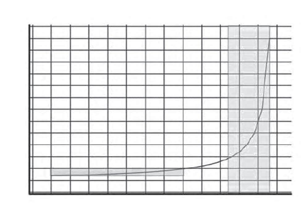
Finally, we should note that everything on climate feedbacks and sensitivity summarized here is based on the assumption that the feedbacks are linear – that is, CO2 and other feedbacks are linearly dependent on the temperature response. But the Earth’s climate system is highly nonlinear in many ways, and can even be considered chaotic (showing apparently random behavior) in a mathematical sense. So any calculations of feedback and climate sensitivity should in principle be founded on nonlinear feedback theory.

Inclusion of nonlinear quadratic terms in the analysis of feedbacks from IPCC climate models appears to show signiicant nonlinearities, especially in the feedbacks from high clouds and temperature/altitude (lapse rate).450 his underlines how little is really understood about climate feedbacks.

Figure A.1: CO2 Climate Sensitivity and Feedback

Glossary

AMO the Atlantic Multidecadal Oscillation, a natural climate cycle in the Atlantic Ocean aerosol a suspension of tiny particles in the atmosphere, oten resulting from the burning of fossil fuels

BEST ................ Berkeley Earth Surface Temperature study

cap-and-trade......... a market trading scheme that limits emissions of a toxic pollutant, or of a greenhouse gas such as CO2, into the atmosphere

carbon cap............ the limit imposed on annual CO2 emissions in a capand-trade scheme

CBO ................. U.S. Congressional Budget Oice

Celsius ............... the metric temperature scale

Climategate........... the leaking of thousands of CRU emails and documents onto the Internet in 2009 and 2011; the emails were between top climate scientists over the period from 1996 to 2009

climate sensitivity the response of the Earth’s climate system to a forcing such as solar radiation or added CO2 in the atmosphere; the sensitivity to CO2 is oten measured as the temperature increase caused by a doubling of the CO2 level

CO2..................

carbon dioxide

CRU ................. Climatic Research Unit at the University of East Anglia, UK

DOE ................. U.S. Department of Energy

EIA .................. U.S. DOE Energy Information Administration

El Niño. . . . . . . . . . . . . . . a natural climate cycle that causes temperature luctuations and other climatic efects in tropical regions of the eastern Paciic Ocean; El Niño is the warm phase of the El Niño – Southern Oscillation (ENSO)

ENSO ................ see El Niño

EPA.................. U.S. Environmental Protection Agency

ETS.................. emissions trading scheme; the same as cap-and-trade Fahrenheit............ the U.S. temperature scale feedback.............. a response to a disturbance (forcing) that feeds back to modify the disturbance itself, either magnifying or diminishing it (positive or negative feedback, respectively); “zero” feedback in climatology corresponds to no change in the heat energy normally radiated away by the Earth – a situation that electronics engineers would describe as negative feedback, since heat is still being lost

FOIA ................ U.S. Freedom of Information Act, which gives citizens the right to access federal information, including information about federally funded research programs forcing ............... radiative forcing, which is a disturbance that alters the climate system and that usually gives rise to feedback processes; related to climate sensitivity

fossil fuel ............. a fuel such as coal, oil or natural gas that is produced over millions of years by the decomposition of buried fossils, and that gives of CO2 when burned

GHCN the Global Historical Climatology Network

GISS ................. NASA Goddard Institute for Space Science

greenhouse gas a gas in the atmosphere such as water vapor, CO2, methane or nitrous oxide, all of which can trap heat radiated into space by the Earth; the main greenhouse gas is water vapor

HadCRU ............. the collaboration between the CRU at the University of East Anglia, UK and the UK Met Oice’s Hadley Centre hockey stick .......... the name given to the erroneous IPCC graph published in 2001, showing reconstructed temperatures for the past 1,000 years and resembling a hockey stick on its side

ice age................ an extended period of severe global cooling in the past, lasting for tens or hundreds of thousands of years, when much of the Earth (especially the Northern Hemisphere) was covered by vast ice sheets and glaciers

ice core............... a cylindrical core of ice extracted from an ice sheet by hollow drilling; air bubbles trapped in the ice provide a historical proxy record of past temperatures and CO2 levels

IPCC ................ the UN’s Intergovernmental Panel on Climate Change

Kyoto Protocol ........ a UN protocol to limit emissions of CO2 and other greenhouse gases, through a cap-and-trade system that mandates carbon caps for industrialized countries; the protocol, which has not been ratiied by the U.S., took efect in 2005

La Niña the cool phase of the El Niño – Southern Oscillation (ENSO), oten following the El Niño warm phase

Little Ice Age.......... an unusually cool period, but not as cold as the glacial ice ages in the Earth’s distant past, that lasted from about 1500 to the beginning of modern global warming around 1850

Maunder Minimum ... the period from 1645 to 1715, when the sun’s activity was low and the annual number of sunspots was close to zero

Medieval Warm Period the previous period of global warming, lasting from approximately 800 to 1300

NAM ................ U.S. National Association of Manufacturers

NASA................ U.S. National Aeronautics and Space Administration

GLOBAL WARMING FALSE ALARM

NCDC ............... U.S. National Climatic Data Center, which is part of NOAA

NOAA ............... U.S. National Oceanic and Atmospheric Administration

paleoclimatology the study of past climates, including past climate change

PDO ................. the Paciic Decadal Oscillation, a natural climate cycle in the Paciic Ocean of much longer duration than El Niño and La Niña

RSS .................. Remote Sensing Systems, which analyzes NOAA satellite data to compile the RSS temperature dataset temperature anomaly… the deviation of a particular temperature measurement from the average temperature over a period of time

TSI .................. total solar irradiance, a measure of the sun’s brightness or activity

UAH................. the University of Alabama in Huntsville, which analyzes NOAA satellite data to compile the UAH temperature dataset

urban heat island ...... a term referring to the warmth generated by urban surroundings, such as buildings and concrete, that biases measured temperatures upward

USHCN the U.S. Historical Climatology Network

UV .................. ultraviolet, one of three main types of radiation emitted by the sun (ultraviolet, visible and infrared); UV and visible radiation are shortwave, while infrared is longwave

WMO................ the World Meteorological Organization

Notes and References

Chapter 1: Climate Change Delusions

1 he assumed connection is known as anthropogenic [human-caused] global warming (AGW) in climate science.

2 Steven Goddard, “Quick Flood Facts”, Real Science blog, October 18, 2011, found at http:// www.real-science.com/quick-lood-facts.

3 Judith Curry, “Weather weirding: back to the 1950s”, Climate Etc. blog, September 5, 2011, found at http://judithcurry.com/2011/09/05/weather-weirding-back-to-the-1950s/.

4 Steven Goddard, “New GISS Data Set Heating Up he Arctic”, Real Science blog, January 15, 2012, found at http://www.real-science.com/new-giss-data-set-heating-arctic.

5 A recent book that proiles prominent global warming skeptics is titled he Deniers, in order to emphasize alarmists’ derogatory use of the term – Lawrence Solomon, he Deniers:heWorldRenownedScientistsWhoStoodUpAgainstGlobalWarmingHysteria, Political Persecution, and Fraud (Richard Vigilante Books, 2008).

6 Ray Evans, “he Kyoto Protocol’s Statistical Fallacies”, Quadrant, May 2003; summarized by HighBeam Research at http://www.highbeam.com/doc/1G1-102024975.html.

7 “he Gore Campaign”, 60 Minutes interview by Lesley Stahl, CBS News, March 30, 2008, found at http://www.cbsnews.com/video/watch/?id=3980795n&tag=contentBody;story MediaBox.

8 Pew Research Center found that only 38% of Americans surveyed in November 2011 say global warming is occurring mostly because of human activity, such as the burning of fossil fuels; reported at http://www.people-press.org/2011/12/01/modest-rise-in-numbersaying-there-is-solid-evidence-of-global-warming/?src=rss_main. he other 62% are presumed to be skeptics.

-151-

9 Rasmussen Reports found that only 40% of likely U.S. voters surveyed in January 2012 thinkthatglobalwarmingisprimarilycausedbyhumanactivity;reportedathttp://www. rasmussenreports.com/public_content/politics/current_events/environment_energy/ energy_update. he other 60% are presumed to be skeptics.

10 Hans von Storch and Dennis Bray, “CliSci2008: A Survey of the Perspectives of Climate Scientists Concerning Climate Science and Climate Change”, GKSS report 2010/9, found at http://coast.gkss.de/staf/storch/pdf/GKSS_2010_9.CLISCI.pdf. he sum of responses

1, 2, 3 and ½ of 4 (out of 7 possible responses) to question 21, “How convinced are you that most of recent or near future climate change is, or will be, a result of anthropogenic causes?”, is 13.8%.

11 Peter T. Doran and Maggie Kendall Zimmerman, “Examining the scientiic consensus on climate change”, Eos Transactions AGU 90, pp. 22-23 (2009), available at http://tigger. uic.edu/~pdoran/012009_Doran_inal.pdf.

12 Ibid.

13 Stephen J. Farnsworth and S. Robert Lichter, “Structure of Scientiic Opinion on Climate Change”, International Journal of Public Opinion Research, October 27, 2011; summarized by John Wihbey, Journalist’s Resource at http://journalistsresource.org/ studies/environment/climate-change/structure-scientiic-opinion-climate-change/.

14 William R. L. Anderegg, James W. Prall, Jacob Harold and Stephen H. Schneider, “Expert credibility in climate change”, Proceedings of the National Academy of Sciences 107, pp. 12107-12109 (2010), found at http://www.pnas.org/content/107/27/12107.full.pdf+html.

15 Eli Kintisch, “Scientists ‘Convinced’ of Climate Consensus More Prominent han Opponents, Says Paper”, AAAS ScienceInsider, June 21, 2010, found at http://news. sciencemag.org/scienceinsider/2010/06/scientists-convinced-of-climate.html.

16 U.S. Senate Environment and Public Works Committee (Minority) Report, December 20, 2007, found at http://epw.senate.gov/public/index.cfm?FuseAction=Minority. SenateReport.

17 “More han 1000 International Scientists Dissent Over Man-Made Global Warming Claims: Scientists Continue to Debunk Fading ‘Consensus’ in 2008 & 2009 & 2010”, Climate Depot report, December 8, 2010, found at http://www.climatedepot. com/a/9035/SPECIAL-REPORT-More-Than-1000-International-Scientists-DissentOver-ManMade-Global-Warming-Claims--Challenge-UN-IPCC--Gore.

18 Global Warming Petition Project, Oregon Institute of Science and Medicine, described at http://www.petitionproject.org/.

-152-

NoTESANDREfERENCES

19 Richard S. Lindzen, “Climate of Fear”, he Wall Street Journal, Opinion Journal, April 12, 2006.

20 IPCC, Climate Change 2007: he Physical Science Basis, Chapter 1: Historical Overview of Climate Change Science, Section 1.6.

21 Ibid.

22 IPCC, Climate Change 2007: he Physical Science Basis, Summary for Policymakers.

23 For an explanation of greenhouse gases, see the next section “he CO2 Global Warming Hypothesis” in this chapter.

24 IPCC, 2007, at http://www.ipcc.ch/pdf/press-ar4/ipcc-lyer-low.pdf.

25 John McLean, “he IPCC can’t count its ‘expert scientists’: Author and reviewer numbers are wrong”, January 18, 2009, found at http://mclean.ch/climate/docs/IPCC_numbers. pdf.

26 According to John McLean (in Reference 25 above), the IPCC’s total of 3,750 authors and reviewers falls to 2,890 when duplicate names are removed. Multiplying the estimated 2,000 climate scientists by the ratio (2,890/3,750) gives an estimate of 1,541 climate scientists.

27 HadCRUT3 global combined land and sea surface temperature record, from http:// www.cru.uea.ac.uk/cru/info/warming/. he Climatic Research Unit (CRU) is part of the University of East Anglia in the UK, and compiles the temperature record jointly with the UK Met Oice Hadley Centre, the collaboration being known as HadCRU.

28 Slide5athttp://climateprediction.net/schools/docs/correlation_causation.ppt#257,5,Data for last 150 years.

29 IPCC, Climate Change 2007: he Physical Science Basis, Summary for Policymakers, p. 5. Although there is general agreement that warming has occurred, the exact amount of the temperature increase has been disputed, as discussed in Chapter 2: Science Gone Wrong of this book. As well as the temperature increase itself, the rate of temperature increase since 1980 is in dispute. If the increase is smaller than 0.8o Celsius (1.4o Fahrenheit), the CO2 hypothesis is less likely to be valid. But in any case, the hypothesis is invalidated by the three red lags for CO2 that are listed in the lower part of Table 1.2.

30 Today’s (2012) CO2 level in the atmosphere is 393 parts per million. his is 40% higher than its assumed preindustrial level in the 1700s, which was 280 parts per million according to the IPCC (in Reference 29 above, p. 2), or about 37% higher than in 1850. CO2 data is always taken from locations well away from forests and other vegetation,

-153-

which temporarily generate CO2 from overnight respiration, and far from any industrial activity.

31 See Chapter 4: CO2 Sense and Sensitivity.

32 Solar radiation is absorbed and radiated by the Earth and its atmosphere in two diferent wavelength regions: absorption takes place at short (ultraviolet and visible) wavelengths, while heat is radiated away at long (infrared) wavelengths. Greenhouse gases in the atmosphere allow most of the incoming shortwave radiation to pass through, but absorb a substantial portion of the outgoing longwave radiation.

33 Svante Arrhenius, “Die vermutliche ursache der klimaschwankungen”, Meddelanden från K. Vetenskapsakademiens Nobelinstitut 1, pp. 1–10 (1906).

34 he atmosphere on Venus, which is very dense, consists of 97% CO2. his near immersion of the planet in CO2 contributes to the high and inhospitable surface temperature there of around 470o Celsius (880o Fahrenheit), though some of the greenhouse warming on Venus comes from thick banks of sulfuric acid clouds sitting above the CO2

35 Responses to questions 11c and 11d in Reference 10 above.

36 Sunspots are small dark spots on the sun’s surface which come from magnetic storms, and which can be seen through a ilter on a telescope.

37 Cosmic rays are highly energetic charged particles, most of which originate in the shock waves of supernova explosions that occur far away in our galaxy.

38 IPCC, Climate Change 2007: he Physical Science Basis, Chapter 1: Historical Overview of Climate Change Science, Section 1.4.3.

Chapter 2: Science Gone Wrong

39 IPCC, Climate Change 2007: he Physical Science Basis, Chapter 1: Historical Overview of Climate Change, Section 1.2.

40 he scientiic method consists of six basic steps: (1) Observation or data gathering; (2) Formulation of a hypothesis, which is an educated guess, to explain the observations;

(3) Initial testing of the hypothesis by experiment; (4) Further, independent testing if the hypothesis is veriied by the initial tests; (5) Elevation of the hypothesis, or several hypotheses, to a theory (based on a limited number of observations) or a law (based on many observations); (6) Modiication or rejection of any hypothesis or theory if contrary observations are made at any stage. In formulating hypotheses, two of the standard reasoning processes used are induction and deduction. Induction reasons from a particular case to a general conclusion, while deduction reasons from general

evidence to a particular conclusion – the CO2 hypothesis is an example of deduction. An important element of the scientiic method is the falsiiability criterion, which says that a single contrary observation can invalidate a whole theory or law (though not generally a hypothesis).

41 IPCC, Climate Change 2007: he Physical Science Basis, Chapter 1: Historical Overview of Climate Change Science, Section 1.3.3.

42 Bias, a statistician’s term, is known as systematic error in scientiic parlance.

43 ForexamplesintheU.S.,seeS.A.Changnon,“Ararelongrecordofdeepsoiltemperatures deines temporal temperature changes and an urban heat island”, Climatic Change 38, pp. 113-128 (1999); and Jim Goodridge, slide 10 in “Impact of Climate Variation on Flood Control Planning in California”, presentation at California Weather Symposium, Sierra College, Rocklin, CA, June 26, 1999, found at http://cepsym.info/Sympro1999/goodridge. pdf.

44 Anthony Watts, “Is the U.S. Surface Temperature Record Reliable?”, Chicago, IL: he Heartland Institute, 2009. his is part of ongoing work in the Surface Stations Project; the project is cataloged at http://www.surfacestations.org/, and the 2009 report is available at Watts Up With hat blog, http://wattsupwiththat.iles.wordpress.com/2009/05/ surfacestationsreport_spring09.pdf.

45 Ibid.

46 Souleymane Fall, Anthony Watts, John Nielsen‐Gammon, Evan Jones, Dev Niyogi, John R. Christy and Roger A. Pielke Sr., “Analysis of the impacts of station exposure on the U.S. Historical Climatology Network temperatures and temperature trends”, Journal of Geophysical Research 116, p. D14120 (2011), found at http://pielkeclimatesci.iles. wordpress.com/2011/07/r-367.pdf.

47 he upward bias in U.S. Historical Climatology Network (USHCN) temperatures is estimated by Fall et al (in Reference 46 above) as 0.3o Celsius (0.5o Fahrenheit), at the poorest station sites compared to the best sites. he poorest and best sites from the Surface Stations Project that were chosen for the analysis number 61 and 80 stations, respectively. Multiplying the estimated bias for the poorest sites of 0.3o Celsius (0.5o Fahrenheit) by the fraction of poor sites (61/141) yields an overall bias of 0.13o Celsius (0.23o Fahrenheit).

48 MatthewJ.Menne,ClaudeN.WilliamsJr.andMichaelA.Palecki,“Onthereliabilityofthe U.S. surface temperature record”, Journal of Geophysical Research 115, p. D11108 (2010), found at http://www1.ncdc.noaa.gov/pub/data/ushcn/v2/monthly/menne-etal2010.pdf. he routine adjustments to USHCN raw data, which are known as homogenization,

-155-

supposedly correct temperatures for changes introduced by the switch in the 1980s from older liquid-in-glass thermometers to newer electronic sensors, and for station siting changes.

49 Ross R. McKitrick and Patrick J. Michaels, “A test of corrections for extraneous signals in gridded surface temperature data”, Climate Research 26, pp. 159–173 (2004) and Erratum, Climate Research 27, pp. 265– 268 (2004), both available at http://www. uoguelph.ca/~rmckitri/research/gdptemp.html; and “Quantifying the inluence of anthropogenic surface processes and inhomogeneities on gridded global climate data”, Journal of Geophysical Research 112, p. D24S09 (2007), found at http://www.uoguelph. ca/~rmckitri/research/jgr07/M&M.JGRDec07.pdf.

50 IPCC, Climate Change 2007: he Physical Science Basis, Chapter 3: Observations: Surface and Atmospheric Climate Change, Section 3.2.2.2.

51 he IPCC (in Reference 50 above, Executive Summary) claims that the global warming ratefromurbanheatislandsisonly0.006o Celsius(0.01o Fahrenheit)perdecade,compared with the overall land surface warming rate since 1980 of 0.27o Celsius (0.49o Fahrenheit) per decade – or a negligible 2.2%. his contrasts with the estimate made by McKitrickand Michaels(in Reference49above)thattheurbanheat islandefectcontributes 0.14o Celsius (0.25o Fahrenheit) of the 0.27o Celsius (0.49o Fahrenheit) per decade warming rate – more than 50% of the measured global warming rate on land.

52 McKitrick and Michaels (in Reference 49 above) estimate that the land surface warming rate since 1980 falls from the IPCC’s value of 0.27o Celsius (0.49o Fahrenheit) per decade to 0.13o Celsius (0.23o Fahrenheit) per decade, when urban heat islands are taken into account. his land warming rate can be combined with the IPCC ocean warming rate of 0.13o Celsius (0.23o Fahrenheit) per decade, which is the same value, to give a corrected post-1980 global warming rate also equal to 0.13o Celsius (0.23o Fahrenheit) per decade. his is 24% lower than the IPCC global warming rate of 0.17o Celsius (0.31o Fahrenheit) per decade. he IPCC warming rates (from Reference 50 above, Executive Summary) are weighted averages over the Northern and Southern Hemispheres.

53 he BEST study maintains that the global urban heating rate over the period 1950-2010 was -0.19 ± 0.19o Celsius (-0.34 ± 0.34o Fahrenheit) per century, a result that is consistent with either zero or a small negative efect. See “Inluence of Urban Heating on the Global Temperature Land Average Using Rural Sites Identiied from MODIS Classiications”, and also “Earth Atmospheric Land Surface Temperature and Station Quality in the United States”, at http://berkeleyearth.org/available-resources/.

NoTESANDREfERENCES

54 Roger Pielke Sr., “Erroneous Information in the Report ‘Procedural Review of EPA’s Greenhouse Gases Endangerment Finding Data Quality Processes’ ”, Climate Science: Roger Pielke Sr. blog, October 5, 2011, found at http://pielkeclimatesci.wordpress. com/2011/10/05/erroneous-information-in-the-report-procedural-review-of-epasgreenhouse-gases-endangerment-inding-data-quality-processes/.

55 “Do Judith Curry and Richard Muller disagree?”, reported by Watts Up With hat blog, November 13, 2011, at http://wattsupwiththat.com/2011/11/13/the-waxman-markeycircus-is-coming-to-town-dr-richard-muller-to-showcase-best-under-the-bigtop/.

56 “Decadal Variations in the Global Atmospheric Land Temperatures”, Berkeley Earth Surface Temperature study, found at http://berkeleyearth.org/available-resources/.

57 Roy W. Spencer, “Latest Global Temps”, updated monthly at http://www.drroyspencer. com/latest-global-temperatures/.hegraphshowstheNOAAglobalsatellitetemperature record for the lower troposphere, which is the layer of the atmosphere closest to the Earth’s surface, compiled at the University of Alabama in Huntsville (UAH); another compilation of the same record is produced by Remote Sensing Systems (RSS).

58 UAH global land and sea surface satellite temperature record up to July 2012, reported at http://vortex.nsstc.uah.edu/data/msu/t2lt/uahncdc.lt. For the RSS dataset, found at http://www.ssmi.com/msu/msu_data_description.html#msu_amsu_time_series, the reported global warming rate to July 2012 was 0.13o Celsius (0.23o Fahrenheit) per decade.

59 IPCC, Climate Change 2007: he Physical Science Basis, Chapter 3: Observations: Surface and Atmospheric Climate Change, Executive Summary.

60 A. Sánchez-Lugo, J. J. Kennedy and P. Berrisford: [Global Climate] Temperatures in “State of the Climate in 2010”, Bulletin of the American Meteorological Society 92, p. S36 (2011), found at http://www.ncdc.noaa.gov/bams-state-of-the-climate/2010.php.

61 “he world is hotter than ever – NOAA”, ICECAP NOTE: UAH RELEASE, International Climate and Environmental Change Assessment Project (ICECAP) blog, July 16, 2010, found at http://icecap.us/index.php/go/joes-blog/the_world_is_hotter_than_ever_ noaa2/.

62 NOAANationalClimaticDataCenter(NCDC),“GlobalSurfaceTemperatureAnomalies”, found at http://www.ncdc.noaa.gov/cmb-faq/anomalies.php. he NCDC temperature record is part of the Global Historical Climatology Network (GHCN) database.

63 Anthony Watts, “New study shows half of the global warming in the USA is artiicial”, Watts Up With hat blog, July 29, 2012, found at http://wattsupwiththat.com/2012/07/29/ press-release-2/.henewmethodologywaspioneeredbyMichelLeroyofMETEOFrance,

-157-

and utilizes the surface area – rather than just the distance – of heat sinks and sources near temperature sensors, in order to gauge their impact on temperature measurements. See also “An area and distance weighted analysis of the impacts of station exposure on the U.S. Historical Climatology Network temperatures and temperature trends’, a paper submitted for publication, at http://wattsupwiththat.iles.wordpress.com/2012/07/wattset-al_2012_discussion_paper_webrelease.pdf.

64 Ibid.

65 Craig Loehle and J. Huston McCulloch, “Correction to: A 2000-year global temperature reconstruction based on non-tree ring proxies”, Energy & Environment 19, pp. 93-100 (2008), found at http://www.ncasi.org/publications/Detail.aspx?id=3025. he proxies used in this reconstruction included ocean sediments, boreholes, pollen, and cave stalagmites.

66 IPCC, Climate Change 2007: he Physical Science Basis, Figure 6.4 and FAQ 2.1, Figure 1.

67 MichaelE.Mann,RaymondS.BradleyandMalcolmK.Hughes,“Global-scaletemperature patterns and climate forcing over the past six centuries”, Nature 392, pp. 779-787 (1998), found at http://www.geo.umass.edu/faculty/bradley/mann1998.pdf; and “Northern Hemisphere temperatures during the past millennium: Inferences, uncertainties, and limitations”, Geophysical Research Letters 26, pp. 759-762 (1999), found at http://www. ncdc.noaa.gov/paleo/pubs/millennium-camera.pdf.

68 IPCC, Climate Change 2001: he Scientiic Basis, Figure 2.20.

69 IPCC, Climate Change 1990: Scientiic Assessment of Climate Change, Figure 7.1(c).

70 As well as tree ring sensitivity to factors such as moisture and CO2, this is partly because of divergence – a mathematical term that refers to trees showing a positive growth response to warming in a past calibration period, but a lesser or even negative response in recent times. For a discussion, see Craig Loehle, “A mathematical analysis of the divergence problem in dendroclimatology”, Climatic Change 94, pp. 233–245 (2009), available at http://icecap.us/images/uploads/Loehle_Divergence_CC.pdf

71 Mann et al (in Reference 67 above) ignored tree-ring data from 1980 onwards, while other studies excluded it ater about 1960.

72 Stephen McIntyre and Ross McKitrick, “Corrections to the Mann et. al. (1998) proxy data base and Northern Hemispheric average temperature series”, Energy & Environment 14, pp. 751-771 (2003), found at http://www.uoguelph.ca/~rmckitri/research/MM03.pdf; and “Hockey Sticks, Principal Components and Spurious Signiicance”, Geophysical

-158-

NoTESANDREfERENCES

Research Letters 32, p. L03710 (2005), found at http://climateaudit.iles.wordpress. com/2009/12/mcintyre-grl-2005.pdf. Both papers are discussed further at http://www. uoguelph.ca/~rmckitri/research/MM-W05-background.pdf.

73 Ibid; principal components is a statistical term.

74 Edward J. Wegman, David W. Scott and Yasmin H. Said, U.S. House Committee on Energy and Commerce Ad Hoc Committee Report on the ‘Hockey Stick’ Global Climate Reconstruction, July 19, 2006, found at http://www.uoguelph.ca/~rmckitri/research/ WegmanReport.pdf.

75 Surface Temperature Reconstructions for the Last 2,000 Years (National Academies Press, 2006), Executive Summary, found at http://www.nap.edu/catalog/11676.html.

76 See, for example, S. Fred Singer and Dennis T. Avery, Unstoppable Global Warming: Every 1,500 Years (Rowman & Littleield, 2nd edition, 2008), pp. 46-92.

77 Michael E. Mann, Zhihua Zhang, Malcolm K. Hughes, Raymond S. Bradley, Sonya K. Miller, Scott Rutherford and Fenbiao Ni, “Proxy-based reconstructions of hemispheric and global surface temperature variations over the past two millennia”, Proceedings of the National Academy of Sciences 105, pp. 13252–13257 (2008), found at http://www.pnas. org/content/early/2008/09/02/0805721105.full.pdf+html. he proxies used in the new reconstruction included ice cores, lake sediments, corals, and cave stalagmites.

78 Richard Black, “Climate ‘hockey stick’ is revived”, found at http://news.bbc.co.uk/2/hi/ science/nature/7592575.stm.

79 Stephen McIntyre and Ross R. McKitrick, “Proxy inconsistency and other problems in millennial paleoclimate reconstructions”, Proceedings of the National Academy of Sciences 106, p. E10 (2009), found at http://www.pnas.org/content/106/6/E10.full.

80 Keith R. Brifa, Vladimir V. Shishov, homas M. Melvin, Eugene A. Vaganov, Håken Grudd, Rashit M. Hantemirov, Matti Eronen and Muktar M. Naurzbaev, “Trends in recenttemperatureandradialtreegrowthspanning2000yearsacrossnorthwestEurasia”, PhilosophicalTransactionsoftheRoyalSociety B363, pp. 2269-2282 (2008), found at http:// rstb.royalsocietypublishing.org/content/363/1501/2269.full.

81 Stephen McIntyre, “YAD06 – the Most Inluential Tree in the World”, Watts Up With hat blog, October 1, 2009, found at http://wattsupwiththat.com/2009/10/01/mirrorposting-yad06-the-most-inluential-tree-in-the-world/.

82 LiuYu,CaiQiuFang,SongHuiMing,AnZhiShengandHansW.Linderholm,“Amplitudes, rates, periodicities and causes of temperature variations in the past 2485 years and future trends over the central-eastern Tibetan Plateau”, Chinese Science Bulletin 56, pp. 2986-

-159-

GLOBAL WARMING FALSE ALARM

2994 (2011), found at http://csb.scichina.com:8080/kxtbe/EN/volumn/volumn_6268. shtml#.

83 IPCC, Climate Change 2007: he Physical Science Basis, Chapter 6: Palaeoclimate, Box 6.4 and Section 6.6.1.1.

84 David Deming, “Global warming, the politicization of science, and Michael Crichton’s State of Fear”, Journal of Scientiic Exploration 19, no. 4 (2005), found at http://www. mitosyfraudes.org/Polit/Deming.html.

85 Ibid.

86 James Hansen, Reto Ruedy, Jay Glascoe and Makiko Sato, “Whither U.S. Climate?”, NASA GISS Science Briefs, August 1999, found at http://www.giss.nasa.gov/research/ briefs/hansen_07/.

87 NASA GISS Surface Temperature Analysis, “Annual Mean Temperature Change in the United States”, found at http://data.giss.nasa.gov/gistemp/graphs_v3/.

88 An animated version of Figure 2.6, showing the switch in hottest year from 1934 to 1998, can be viewed at http://wattsupwiththat.iles.wordpress.com/2012/03/1998changesanno tated1.gif.

89 Glenn Elert, “Hottest Temperature on Earth”, he Physics Factbook, at http:// hypertextbook.com/facts/2000/MichaelLevin.shtml.

90 “ClimateofthePhilippines”,athttp://en.wikipedia.org/wiki/Climate_of_the_Philippines.

91 Matthew J. Menne, Claude N. Williams Jr. and Russell S. Vose, “he U.S. Historical Climatology Network Monthly Temperature Data, Version 2”, Bulletin of the American Meteorological Society 90, pp. 993-1107 (2009), available at tp://tp.ncdc.noaa.gov/pub/ data/ushcn/v2/monthly/menne-etal2009.pdf. See also Reference 48 above.

92 Louise Gray, “Met Oice: World warmed even more in last ten years than previously thought when Arctic data added”, he Telegraph, March 19, 2012, found at http://www. telegraph.co.uk/earth/earthnews/9153473/Met-Oice-World-warmed-even-more-inlast-ten-years-than-previously-thought-when-Arctic-data-added.html.

93 Climategate email 0938018124.txt, found at ClimateGate FOIA Grepper, http://www. ecowho.com/foia.php?ile=0938018124.txt.

94 Climategate email 3451.txt, found at ClimateGate FOIA Grepper, http://www.ecowho. com/foia.php?ile=3451.txt.

95 Climategate email 1054736277.txt, found at ClimateGate FOIA Grepper, http://www. ecowho.com/foia.php?ile=1054736277.txt.

-160-

NoTESANDREfERENCES

96 Climategate email 1076359809.txt, found at ClimateGate FOIA Grepper, http://www. ecowho.com/foia.php?ile=1076359809.txt.

97 Climategate email 1107454306.txt, found at ClimateGate FOIA Grepper, http://www. ecowho.com/foia.php?ile=1107454306.txt.

98 Climategate email 1109021312.txt, found at ClimateGate FOIA Grepper, http://www. ecowho.com/foia.php?ile=1109021312.txt.

99 Climategate email 1147435800.txt, found at ClimateGate FOIA Grepper, http://www. ecowho.com/foia.php?ile=1147435800.txt.

100 Douglas J. Keenan, “he fraud allegation against some climatic research of Wei-Chyung Wang”, Energy & Environment 18 , pp. 985-995 (2007), summarized and updated at http://www.informath.org/apprise/a5620.htm.

101 Wei-Chyung Wang, Zhaomei Zeng and homas R. Karl, “Urban heat islands in China”, Geophysical Research Letters 17, pp. 2377–2380 (1990), found at http://www.informath. org/apprise/a5620/b23.pdf.

102 P. D. Jones, P. Y. Groisman, M. Coughlan, N. Plummer, W.-C. Wang and T. R. Karl, “Assessment of urbanization efects in time series of surface air temperature over land”, Nature 347, pp. 169–172 (1990), found at http://www.informath.org/apprise/a5620/b90. pdf.

103 Douglas J. Keenan (February 2010), at http://www.informath.org/apprise/a5620/b17.htm.

104 IPCC, Climate Change 2007: he Physical Science Basis, Chapter 3: Observations: Surface and Atmospheric Climate Change, Section 3.2.2.2. Phil Jones, lead author of Reference 102 above, was also one of the two lead authors of this IPCC report chapter.

105 Fred Pearce, “Strange case of moving weather posts and a scientist under siege”, he Guardian, February 1, 2010, found at http://www.guardian.co.uk/environment/2010/ feb/01/dispute-weather-fraud.

106 Climategate email 2655.txt, found at ClimateGate FOIA Grepper, http://www.ecowho. com/foia.php?ile=2655.txt.

107 Climategate email 1177163150.txt, found at ClimateGate FOIA Grepper, http://www. ecowho.com/foia.php?ile=1177163150.txt.

108 P.D.Jones,D.H.ListerandQ.Li,“Urbanizationefectsinlarge-scaletemperaturerecords, with an emphasis on China”, Journal of Geophysical Research 113, p. D16122 (2008). he study concludes that urban-related warming in China during the period 1951–2004 was about 0.1o Celsius (0.2o Fahrenheit) per decade, which is 17 times larger than the IPCC’s estimated warming rate from urban heat islands (in Reference 104 above, Executive

-161-

Summary). Over 5.4 decades, this amounts to a contribution from urbanization of 0.54o Celsius (0.97o Fahrenheit). he contribution is two thirds of the true climatic warming in China of 0.81o Celsius (1.5o Fahrenheit) over the same period.

109 Judith Curry, “On the credibility of climate research”, November 22, 2009, found at http:// camirror.wordpress.com/2009/11/22/curry-on-the-credibility-of-climate-research/.

110 Clive Cook, “Climategate and the Big Green Lie”, he Atlantic, July 14, 2010, found at http://www.theatlantic.com/politics/archive/2010/07/climategate-and-the-big-greenlie/59709/.

111 Report of he Independent Climate Change E-mails Review, July 2010, found at http:// www.cce-review.org/.

112 McKitrick and Michaels (in Reference 49 above) estimated a global warming rate on land of 0.14o Celsius (0.25o Fahrenheit) per decade from urban heat islands alone. he IPCC (in Reference 50 above) also dismisses another study that estimated the contribution of urbanization and other changes in land use at 0.09o Celsius (0.16o Fahrenheit) per decade in the U.S. [Eugenia Kalnay & Ming Cai, “Impact of urbanization and land-use change on climate”, Nature 423, pp. 528-531 (2003), found at http://www.warwickhughes.com/ climate/kalnay.pdf].

113 Ross R. McKitrick and Patrick J. Michaels, Background Discussion on “Quantifying the inluence of anthropogenic surface processes and inhomogeneities on gridded global climate data”, found at http://www.uoguelph.ca/~rmckitri/research/jgr07/M&M.JGR07background.pdf.

114 Ibid.

115 IPCC, Climate Change 2007: he Physical Science Basis, Expert and Government Review Comments on the Second-Order Drat, Chapter 3, No. 3-285, found at http://pds.lib. harvard.edu/pds/view/7786376?n=38&imagesize=1200&jp2Res=.25.

116 Ross R. McKitrick, “Atmospheric oscillations do not explain the temperatureindustrialization correlation”, Social Science Research Network, available at: http:// papers.ssrn.com/sol3/papers.cfm?abstract_id=1166424.

117 Climategate email 1089318616.txt, found at ClimateGate FOIA Grepper, http://www. ecowho.com/foia.php?ile=1089318616.txt.

118 Climategate email 2469.txt, found at ClimateGate FOIA Grepper, http://www.ecowho. com/foia.php?ile=2469.txt.

119 Climategate email 3052.txt, found at ClimateGate FOIA Grepper, http://www.ecowho. com/foia.php?ile=3052.txt.

-162-

NoTESANDREfERENCES

120 “Concerned Scientists Reply on Global Warming”, he Wall Street Journal, February 21, 2012, found at http://online.wsj.com/article/SB1000142405297020364600457721324408 4429540.html.

121 See, for example, “Soon and Baliunas controversy”, at http://en.wikipedia.org/wiki/ Soon_and_Baliunas_controversy.

122 Climategate email 1106322460.txt, found at ClimateGate FOIA Grepper, http://www. ecowho.com/foia.php?ile=1106322460.txt.

123 Roy W. Spencer and William D. Braswell, “On the Misdiagnosis of Surface Temperature Feedbacks from Variations in Earth’s Radiant Energy Balance”, Remote Sensing 3, pp. 1603-1613 (2011), found at http://www.mdpi.com/2072-4292/3/8/1603/pdf.

124 Richard Monastersky, “Cool climate paper sinks journal editor”, Nature News blog, September 2, 2011, found at http://blogs.nature.com/news/2011/09/cool_climate_paper_ sinks_journ.html.

125 Wolfgang Wagner, Editorial, “Taking Responsibility on Publishing the Controversial Paper ‘On the Misdiagnosis of Surface Temperature Feedbacks from Variations in Earth’s Radiant Energy Balance’ by Spencer and Braswell”, Remote Sensing 3, pp. 20022004 (2011), found at http://www.mdpi.com/2072-4292/3/9/2002/pdf.

126 IPCC, Appendix A to the Principles Governing IPCC Work (amended November 2003), Section 4.2, found at http://www.ipcc.ch/pdf/ipcc-principles/ipcc-principles-appendix-a. pdf.

127 “he exact changes to 1995 IPCC report: the crucial chapter 8 for the ‘Summary for Policymakers’ ”, found at http://www.greenworldtrust.org.uk/Science/Social/IPCC95-Ch8.htm.

128 Frederick Seitz, “A Major Deception on Global Warming”, he Wall Street Journal, June 12, 1996.

129 Editorial, “Climate debate must not overheat”, Nature 381, p. 539 (1996), available at http:// www.albany.edu/~scifraud/data/sci_fraud_3779.html.

130 Paul N. Edwards and Stephen H. Schneider, “he 1995 IPCC Report: Broad Consensus or ‘Scientiic Cleansing’?”, Ecofable/Ecoscience 1, pp. 3-9 (1997), found at http://pne.people. si.umich.edu/PDF/ecofables.pdf.

131 InterAcademy Council, “Climate change assessments: Review of the processes and procedures of the IPCC”, Report by the Committee to Review the IPCC, October 2010, found at http://reviewipcc.interacademycouncil.net/report.html.

-163-

132 Donna Laframboise, “UN’s Climate Bible Gets 21 ‘F’s on Report Card”, NOconsensus.org blog, April 14, 2010, found at http://www.noconsensus.org/ipcc-audit/indings-mainpage.php.

Chapter 3: Computer Snake Oil?

133 IPCC, Climate Change 2007: he Physical Science Basis, Chapter 1: Historical Overview of Climate Change, Section 1.2.

134 CCSP, “Climate Models: An Assessment of Strengths and Limitations”, Report by the U.S. Climate Change Science Program and the Subcommittee on Global Change Research, Department of Energy (DOE), Oice of Biological and Environmental Research, 2008, Section 1.2, found at http://www.climatescience.gov/Library/sap/sap3-1/inal-report/ sap3-1-inal-all.pdf.

135 Examples of processes or quantities represented by adjustable parameters in climate models include lows of the atmosphere and oceans; atmospheric turbulence near the earth’s surface (in the so-called boundary layer); the relative humidity threshold for cloud formation (separate sets of parameters for low-level and high-level clouds); the eiciency of precipitation evaporation; aerosol microphysics; ocean salinity; sea-ice dynamics; and many more.

136 Quoted by Freeman Dyson in “A meeting with Enrico Fermi”, Nature 427, p. 297 (2004); see http://www.cds.caltech.edu/~murray/books/AM08/pdf/am08-modeling_19Jul11. pdf.

137 James M. Murphy, David M. H. Sexton, David N. Barnett, Gareth S. Jones, Mark J. Webb, Matthew Collins and David A. Stainforth, “Quantiication of modelling uncertainties in a large ensemble of climate change simulations”, Nature 430, pp. 768-772 (2004), found at http://climateprediction.net/science/pubs/nature_murphy_02771.pdf.

138 IPCC, Climate Change 2001: he Scientiic Basis, Chapter 8: Model Evaluation, Table 8.1.

139 IPCC, Climate Change 2007: he Physical Science Basis, Chapter 8: Climate Models and heir Evaluation, Table 8.1.

140 Global energy balance refers to the balance between the amount of absorbed sunlight at the top of the atmosphere and the amount of energy that the Earth radiates away to space, both of which are estimated to be 235-240 W/m2 (watts per square meter) when averaged over a year. It is this balance that is believed to keep our planet at a constant average temperature over the short term. Computer climate models are tuned by adjusting parameters, typically for clouds, to maintain this energy balance. However, because

-164-

NoTESANDREfERENCES

235-240 W/m2 is only an inexact theoretical calculation, the tuning procedure is also subject to uncertainty. his uncertainty can afect the model’s ability to predict climate sensitivity, as discussed by F. A.-M. Bender [F. A.-M. Bender, “A note on the efect of GCM tuning on climate sensitivity”, Environmental Research Letters 3, pp. 1-6 (2008), found at http://www.iop.org/EJ/article/1748-9326/3/1/014001/erl8_1_014001.html].

141 Section 2.5.2 in Reference 134 above, discussing the Community Climate System Model – one of the major classes of climate model used by IPCC modelers.

142 As described in IPCC, Climate Change 2007: he Physical Science Basis, Chapter 8: Climate Models and heir Evaluation.

143 Kesten C. Green and J. Scott Armstrong, “Global warming: Forecasts by scientists versus scientiic forecasts”, Energy & Environment 18 , pp. 997-1021 (2007), found at http://www. forecastingprinciples.com/iles/WarmAudit31.pdf.

144 Ibid.

145 he main uses of adjustable cloud parameters are to approximate cloud formation and dissipation for cirrus (high-level) and stratus clouds; cumulus (low-level) cloud convection, in both fair weather and thunderstorms; turbulence; and conversions between cloud water, rainwater, ice crystals, and snow.

146 “Cloud-resolving models”, which have grid boxes less than a few kilometers square, are already available, but take too long to run even on supercomputers today. hese models can simulate features such as deep updrats and downdrats, cirrus anvil clouds, and aerosol-cloud interactions better than present-day climate models, though still require parameterization of many subgrid-scale processes.

147 J. Hansen et al, “Climate simulations for 1880–2003 with GISS model E”, Climate Dynamics 29, pp. 661–696 (2007), found at http://pubs.giss.nasa.gov/docs/2007/2007_ Hansen_etal_3.pdf. W/m2 (watts per square meter) is a unit of radiative energy; hPa (hectopascals) is a unit of atmospheric pressure identical to mb (millibars), standard atmospheric pressure at sea level being 1013 hPa or 1013 mb.

148 United Nations Framework Convention on Climate Change (UNFCCC), Convention Text (1992), Article 2, found at http://unfccc.int/resource/docs/convkp/conveng.pdf.

149 IPCC, Climate Change 2007: he Physical Science Basis, Chapter 8: Climate Models and heir Evaluation, FAQ 8.1.

150 Ibid, Section 8.6.3.2.

151 IPCC, Climate Change 2007: he Physical Science Basis, Chapter 10: Global Climate Projections, Section 10.2.1.3 and Figure 10.11(a).

-165-

152 IPCC, Climate Change 2007: he Physical Science Basis, Chapter 9: Understanding and Attributing Climate Change, Table 9.4.

153 Claire L. Parkinson, Coming Climate Crisis? Consider the Past, Beware the Big Fix (Rowman & Littleield, reprinted 2012), Chapter 10.

154 Speciically, the troposphere – the lowest layer of the atmosphere

155 IPCC, Climate Change 2007: he Physical Science Basis, Chapter 9: Understanding and Attributing Climate Change, Section 9.2.2.1. Figure 9.1 (c) for well-mixed greenhouse gases, principally CO2, shows a model warming rate of approximately 1.1o Celsius (2.0o Fahrenheit) per century from 1890 to 1999 at an altitude of 10 kilometers (6 miles), and a rate of approximately 0.5o Celsius (0.9o Fahrenheit) per century at ground level. he interval from 1890 to 1999 includes several global warming and cooling periods.

156 B.D.Santer,J.E.PennerandP.W.horne,“Howwellcantheobservedverticaltemperature changes be reconciled with our understanding of the causes of these changes?”, in CCSP, “Temperature Trends in the Lower Atmosphere: Steps for Understanding and Reconciling Diferences”, Report by the U.S. Climate Change Science Program and the Subcommittee on Global Change Research, 2006, found at http://www.climatescience. gov/Library/sap/sap1-1/inalreport/sap1-1-inal-chap5.pdf. he observed temperature change pattern in Figure 5.7, panel E shows the absence of any hot spot at an altitude of 10 kilometers (6 miles), during the global warming period from 1979 to 1999.

157 Weather balloon data such as atmospheric temperature and pressure, which indicates altitude, is transmitted back to a ground station by radiosonde as the balloon ascends through the atmosphere.

158 David H. Douglass, John R. Christy, Benjamin D. Pearson and S. Fred Singer, “A comparison of tropical temperature trends with model predictions”, International Journal of Climatology 28, pp. 1693–1701 (2008), found at http://www.pas.rochester. edu/~douglass/papers/Published%20JOC1651.pdf.

159 Ibid. Table III gives the model warming rate for the mid-troposphere (T2) as 0.23o Celsius (0.41o Fahrenheit) per decade, based on simulations by 22 “Climate of the 20th Century” computer models.

160 B. D. Santer et al, “Consistency of modelled and observed temperature trends in the tropical troposphere”, International Journal of Climatology 28, pp. 1703-1722 (2008), found at https://publicafairs.llnl.gov/news/news_releases/2008/NR-08-10-05-article. pdf. Table I gives the model warming rate for the mid-troposphere (T2) as 0.20o Celsius

-166-

NoTESANDREfERENCES

(0.36o Fahrenheit) per decade, based on simulations by 19 “Climate of the 20th Century” computer models.

161 Computer models do not reproduce tropical climate variability. In particular, the models are unable to predict the timing (except for the El Niño warm phase) and climatic efects of either the El Niño-Southern Oscillation (ENSO), which is an ocean-atmosphere cycle occurring at irregular intervals of 2-8 years, or the Paciic Decadal Oscillation (PDO), or the intraseasonal Madden-Julian Oscillation.

162 DavidEvans,“heMissingHotspot”,foundathttp://sciencespeak.com/MissingSignature. pdf.

163 his is one of several positive feedback mechanisms that could enhance global warming in polar regions, if the CO2 hypothesis were valid. he feedback mechanism involves warmth from CO2 melting snow and ice to expose darker surfaces with lower relectivity (albedo). he less relective surfaces absorb more solar heat, enhancing the warming from CO2 alone.

164 IgorV.Polyakov,RomanV.Bekryaev,GenrikhV.Alekseev,UmaS.Bhatt,RogerL.Colony, Mark A. Johnson, Alexander P. Maskshtas and David Walsh, “Variability and Trends of Air Temperature and Pressure in the Maritime Arctic, 1875-2000”, Journal of Climate 16, pp. 2067-2077 (2003), found at http://journals.ametsoc.org/doi/pdf/10.1175/15200442%282003%29016%3C2067%3AVATOAT%3E2.0.CO%3B2.

165 IPCC, Climate Change 2007: he Physical Science Basis, Chapter 8: Climate Models and heir Evaluation, FAQ 8.1.

166 “Northern Sea Route”, Athropolis Facts: Cold, Icy and Arctic, found at http://www. athropolis.com/arctic-facts/fact-nepass.htm. he Northern Sea Route, a shipping lane that hugs the coast of Russia, was established by the former Soviet Union during the Arctic warm spell in the 1930s. But even today, a leet of icebreakers is required to keep the lane open year-round.

167 Paul Homewood, “GHCN Temperature Adjustments Afect 40% Of he Arctic”, Not a Lot of People Know hat blog, March 11, 2012, found at http://notalotofpeopleknowthat. wordpress.com/2012/03/11/ghcn-temperature-adjustments-afect-40-of-the-arctic/.

168 Peter T. Doran et al, “Antarctic climate cooling and terrestrial ecosystem response”, Nature 415, pp. 517-520 (2002), found at http://www.montana.edu/lkbonney/DOCS/ Publications/DoranEtAl2002ClimteCooling.pdf.

169 Eric J. Steig, David P. Schneider, Scott D. Rutherford, Michael E. Mann, Joseino C. Comiso and Drew T. Shindell, “Warming of the Antarctic ice-sheet surface since the

-167-

1957 International Geophysical Year”, Nature 457, pp. 459-462 (2009), found at http:// www.meteo.psu.edu/~mann/shared/articles/SteigetalNature09.pdf, and Corrigendum, Nature 460, p. 766 (2009), found at http://www.nature.com/nature/journal/v460/n7256/ full/nature08286.html.

170 Hu McCulloch, “Steig 2009’s Non-Correction for Serial Correlation”, February 26, 2009, found at http://climateaudit.org/2009/02/26/steig-2009s-non-correction-for-serialcorrelation/. he issue is what statisticians call serial correlation. Because of the limited number of Antarctic weather stations supplying actual temperature data, the much larger number of reconstructed temperatures across the continent are correlated. his correlation increases the statistical errors beyond those reported by Steig et al in their original paper (Reference 169 above). When the correlation is taken into account, as was done in the Corrigendum, the statistical errors for East Antarctica and the continent as a whole become so large that the temperature change over the past 50 years could be as small as zero.

171 Ryan O’Donnell, Nicholas Lewis, Steve McIntyre and Jef Condon, “Improved Methods for PCA-Based Reconstructions: Case Study Using the Steig et al. (2009) Antarctic Temperature Reconstruction”, Journal of Climate 24, pp. 2099-2115 (2011).

172 Ibid,SupportingInformation,foundathttp://www.climateaudit.info/data/odonnell/4%20 20101208%20SI%20Revised.pdf.

173 Tore Hattermann, Ole Anders Nøst, Jonathan M. Lilly and Lars H. Smedsrud, “Two years of oceanic observations below the Fimbul Ice Shelf, Antarctica”, Geophysical Research Letters 39,p.L12605(2012);summarizedbyLewisPage,“Antarcticiceshelvesnotmelting at all, new ield data show”, he Register, Science, June 25, 2012, found at http://www. theregister.co.uk/2012/06/25/antarctic_ice_not_melting/.

174 Sea ice around Antarctica includes both ice shelves, which are thick slabs of glacial ice anchored to the coast, and loating pack ice.

175 NASA Earth Observatory Features, “Antarctic Sea Ice”, found at http://earthobservatory. nasa.gov/Features/WorldOfChange/sea_ice_south.php; and John Turner et al, “Non‐annular atmospheric circulation change induced by stratospheric ozone depletion and its role in the recent increase of Antarctic sea ice extent”, Geophysical Research Letters 36, p. L08502 (2009), found at http://ruby.fgcu.edu/courses/twimberley/EnviroPhilo/Turner. pdf.

176 An animated display of Antarctic sea ice from 1991 to 2012 can be viewed at http://www. youtube.com/watch?v=txpHVm-9rTg.

-168-

NoTESANDREfERENCES

177 IPCC, Climate Change 2007: he Physical Science Basis, Chapter 7: Couplings Between Changes in the Climate System and Biogeochemistry, Section 7.5.2.4. Aerosol particles in the atmosphere tend to remain in the Northern Hemisphere where they are produced, unlike greenhouse gases such as CO2, which quickly become mixed between the two hemispheres.

178 IPCC, Climate Change 2007: he Physical Science Basis, Chapter 3: Observations: Surface and Atmospheric Climate Change, Table 3.3. From 1979 to 2005, the IPCC’s observed warmingratewas0.24o Celsius(0.43o Fahrenheit)perdecadeintheNorthernHemisphere, and 0.09o Celsius (0.16o Fahrenheit) per decade in the Southern Hemisphere.

179 See the plotted graph for the “HADSST2 global sea surface temperature anomaly” data source, WoodForTrees.org blog, at http://woodfortrees.org/plot/hadsst2gl/from:2000. For a summary of ocean heat content analyses from 2003, see Robert S. Knox and David H. Douglass, “Recent Energy Balance of Earth”, International Journal of Geosciences 1, pp. 99-101 (2010), found at http://www.scirp.org/journal/PaperDownload.aspx?paperID

=3446&returnUrl=http%3a%2f%.

180 IPCC, Climate Change 2007: he Physical Science Basis, Chapter 8: Climate Models and heir Evaluation, Section 8.3.2.

Chapter 4: CO

Sense and Sensitivity

181 Typically, between barometric pressure and wind speed – with lower pressure increasing wind low, which drops the pressure more and causes even higher winds, and so on.

182 For water vapor, which is the dominant greenhouse gas in the atmosphere, the idea is that a small increase in atmospheric CO2 warms the Earth slightly via the greenhouse efect. his warming produces more water vapor by evaporation from oceans and lakes, and the extra water vapor then ampliies the warming even more. For clouds, the initial CO2 warmingproducesmorehigh-levelcloudsthatcausefurtherwarming(asopposedtolowlevel clouds that cause cooling). Melting of terrestrial snow and sea ice by CO2 warming exposes darker surfaces such as soil, rock and seawater, which have lower albedo. he less relective surfaces absorb more of the sun’s radiation and thus push temperatures higher. In all three cases, the tiny efect from CO2 acting alone is magniied, according to climate modelers and the IPCC.

183 IPCC, Climate Change 2007: he Physical Science Basis, Chapter 8: Climate Models and heir Evaluation, Section 8.6.2.3. he combined water vapor-lapse rate feedback in IPCC atmosphere-ocean climate models is estimated to be 0.96 W/m2 per oC, compared to the

cloud feedback of 0.69 W/m2 per oC, and the snow and ice feedback of 0.26 W/m2 per oC. All these are positive feedbacks, though the lapse-rate feedback on its own is usually negative (see Reference 188 below)

184 he water vapor feedback, which depends on CO2 through the greenhouse efect, is the strongest feedback in IPCC climate models. However, its strength depends on the assumption that global warming does not change the relative humidity in the lower atmosphere (troposphere), an assumption originally made in a 1979 study known as the Charney Report [“Carbon Dioxide and Climate: A Scientiic Assessment”, National Academy of Sciences Report, 1979, found at http://www.atmos.ucla.edu/~brianpm/ download/charney_report.pdf]. Warming theoretically increases the water vapor concentration (speciic humidity) in the atmosphere, but also increases the saturation level for water vapor, which deines relative humidity. If the relative humidity distribution inthetropospheredoesnotremainconstantaswarmingoccurs,thewatervaporfeedback may be weaker than estimated.

185 A detailed explanation is given in Reference 162 in Chapter 3: Computer Snake Oil?

186 IPCC, Climate Change 2007: he Physical Science Basis, Chapter 7: Couplings Between Changes in the Climate System and Biogeochemistry, Section 7.3.5.

187 Ibid, Section 7.6.

188 Panel on Climate Change Feedbacks, National Research Council, Understanding Climate Change Feedbacks (National Academies Press, 2003), p. 24, found at http://www.nap.edu/ openbook.php?record_id=10850&page=24. he technical term for the rate of decrease of temperature with altitude in the troposphere is the lapse rate. he greenhouse efect for CO2 is enhanced or diminished by a higher or lower lapse rate, respectively, since water vapor in the colder, upper troposphere radiates less heat away from the Earth than water vapor closer to the warmer surface. In the tropics, where temperatures in the troposphere vary most strongly with altitude, the observed lapse rate is close to the moist adiabatic lapse rate and has been found to decrease with increasing surface temperature – so that the lapse rate feedback is negative, at least in the tropics. In most IPCC climate models, the lapse rate feedback is also negative, although it is positive in some models. Because temperature and water vapor changes are so tightly coupled, the positive water vapor feedback is generally combined with the lapse rate feedback.

189 Primarily from NASA’s Terra and Tropical Rainfall Measuring Mission (TRMM) satellites.

NoTESANDREfERENCES

190 Roy W. Spencer, William D. Braswell, John R. Christy and Justin Hnilo, “Cloud and radiation budget changes associated with tropical intraseasonal oscillations”, Geophysical Research Letters 34, p. L15707 (2007), found at http://www.drroyspencer. com/Spencer_07GRL.pdf. he short–term, intraseasonal climate cycle studied was the Madden-Julian Oscillation. he increase in atmospheric temperature from the cool to the warm phase of this oscillation is, over a few weeks, about as large as the average global warming observed since 1850.

191 UniversityofAlabamainHuntsville,“CirrusDisappearance:WarmingMighthinHeatTrapping Clouds”, ScienceDaily, November 2, 2007, found at http://www.sciencedaily. com/releases/2007/11/071102152636.htm. he heat-trapping ability of high-altitude ice clouds exceeds their solar shading efect, which is the dominant feature of low-altitude clouds.

192 RichardS.Lindzen,Ming-DahChouandArthurY.Hou,“DoestheEarthhaveanadaptive infrared iris?”, Bulletin of the American Meteorological Society 82, pp. 417-432 (2001), found at http://journals.ametsoc.org/doi/pdf/10.1175/1520-0477%282001%29082%3C04 17%3ADTEHAA%3E2.3.CO%3B2.

193 NASA’s Aqua satellite.

194 Roy W. Spencer, “Satellite and climate model evidence against substantial manmade climate change”, available at http://www.drroyspencer.com/satellite-and-climate-modelevidence/.

195 RoyW.Spencer,privatecommunication(2009).henegativefeedbackinthissecondstudy was not observed in outgoing longwave (infrared) radiation from the Earth, as it was in the irst study, but rather in relected shortwave (ultraviolet) solar radiation. Spencer says that the satellite observations showed an excellent match with the IPCC climate models in the longwave region, suggesting that the total longwave feedback – which consists of the water vapor, lapse rate and high cloud feedbacks – is weakly positive. But this weak positive feedback is dominated by the strong negative feedback from low clouds in the shortwave region. he possibility of zero or even negative longwave feedback, also based on satellite observations, had been suggested earlier by Piers Forster and Jonathan Gregory [Piers M. de F. Forster and Jonathan M. Gregory, “he climate sensitivity and its components diagnosed from Earth radiation budget data”, Journal of Climate 19, pp. 39-52 (2006), found at http://journals.ametsoc.org/doi/pdf/10.1175/JCLI3611.1].

196 Roger Davies and Matthew Molloy, “Global cloud height luctuations measured by MISR on Terra from 2000 to 2010”, Geophysical Research Letters 39, p. L03701 (2012);

-171-

summarized in “NASA Satellite Finds Earth’s Clouds are Getting Lower”, NASA Jet Propulsion Laboratory News & Features, February 21, 2012, at http://www.jpl.nasa.gov/ news/news.cfm?release=2012-046.

197 See, for example, Reference 123 in Chapter 2: Science Gone Wrong; and A. E. Dessler, “Cloud variations and the Earth’s energy budget”, Geophysical Research Letters 38, p. L19701 (2011), found at http://geotest.tamu.edu/useriles/216/Dessler2011.pdf. According to Spencer and Braswell, cloud feedbacks cannot be easily disentangled from forcings because of the diferent time dependence with temperature of feedbacks, and of forcings such as increased CO2 levels or changes in cloud cover. Feedback occurs almost simultaneouslywiththetemperaturechange,butthetemperatureresponsetoforcinglags behind due to the heat capacity of the oceans. But according to Dessler, cloud feedbacks can be separated from forcings because the forcing from clouds accounts for only a few percent of observed surface temperature changes, at least in his calculations.

198 IPCC, Climate Change 2007: he Physical Science Basis, Chapter 8: Climate Models and heir Evaluation, Section 8.6.3.2.2. In roughly half of the current IPCC climate models, the feedback from low-level tropical clouds in response to global warming is negative, which is the same as found from satellite data in the second University of Alabama study (see Reference 194 above). But the other half of the IPCC models predict positive feedback from low-level clouds, and all models predict net positive feedback from low-level and high-level clouds combined.

199 IPCC, Climate Change 2007: he Physical Science Basis, Chapter 9: Understanding and Attributing Climate Change, Sections 9.2 and 9.6.1.

200 IPCC, Climate Change 2007: he Physical Science Basis, Summary for Policymakers, p. 12.

201 Ibid.

202 Details of these climate sensitivity calculations, and references, are supplied in the Appendix: Climate Feedbacks and Sensitivity.

203 Nicholas Lewis, “he IPCC’s alteration of Forster & Gregory’s model-independent climate sensitivity results”, Climate Etc. blog, July 5, 2011, found at http://judithcurry. com/2011/07/05/the-ipccs-alteration-of-forster-gregorys-model-independentclimate-sensitivity-results/. For a less technical discussion, see Matt Ridley, “Scientiic Heresy”, at http://wattsupwiththat.iles.wordpress.com/2011/11/ridley_rsa_ millar_speech_scientiic_heresy.pdf.

NoTESANDREfERENCES

204 he increase in global surface temperatures since 1850 is 0.6o Celsius (1.1o Fahrenheit) when the urban heat island efect is taken into account, as discussed in Chapter 2: Science Gone Wrong. According to the IPCC (in Reference 200 above, p. 5), the increase since 1850 is 0.8o Celsius (1.4o Fahrenheit).

205 IPCC, Climate Change 2007: he Physical Science Basis, Chapter 9: Understanding and Attributing Climate Change, Section 9.6.4.

206 Dan Pangburn, “Historical Data On Global Warming provided by U.S. Government Agencies”, March 15, 2008, found at http://www.middlebury.net/op-ed/pangburn.html.

207 Speciically,icecoresfromtheRussianVostokstationinEastAntarctica.Pastatmospheric CO2 levels and surface temperatures are determined from ice cores by measuring the air composition and the oxygen 18O to 16O isotopic ratio, respectively, in air bubbles trapped by the ice. However, the measured levels may not be accurate. Because the air isn’t captured until enough snow has accumulated to pack the subsurface snow into ice, the age of the trapped air is less than the age of the surrounding ice, but by an amount that varies with local conditions. his introduces uncertainty into the timescale. And ice-core CO2 levels may be inaccurate due to changes in the composition of the original air caused by complex physical and chemical processes that occur in the packed ice. Even if that is not the case, the CO2 level in Antarctica and Greenland, from where most ice cores are extracted, is somewhat lower than the global average owing to absorption of CO2 by the colder oceans in those regions.

208 Hubertus Fischer, Martin Wahlen, Jesse Smith, Derek Mastroianni and Bruce Deck, “Ice core records of atmospheric CO2 around the last three glacial terminations”, Science 283, pp. 1712-1714 (1999), found at http://epic.awi.de/825/1/Fis1999a.pdf.

209 Nicolas Caillon, Jefrey P. Severinghaus, Jean Jouzel, Jean-Marc Barnola, Jiancheng Kang and Volodya Y. Lipenkov, “Timing of atmospheric CO2 and Antarctic temperature changes across termination III”, Science 299, pp. 1728-1731 (2003), found at http:// icebubbles.ucsd.edu/Publications/CaillonTermIII.pdf.

210 Lowell Stott, Axel Timmermann and Robert hunell, “Southern Hemisphere and deepsea warming led deglacial atmospheric CO2 rise and tropical warming”, Science 318, pp. 435-438 (2007). he amount of CO2 released from or absorbed by the oceans as the temperature rises or falls, respectively, is thought to depend on temperature-induced changes both in CO2 solubility and in ocean mixing processes for CO2

211 Jeremy D. Shakun et al, “Global warming preceded by increasing carbon dioxide concentrations during the last deglaciation”, Nature 484, pp. 49-55 (2012), found at http://

-173-

sciences.blogs.liberation.fr/iles/shakun-et-al.pdf. he proxies used in the temperature reconstruction included ocean and lake sediments, as well as ice cores.

212 See, for example, J. R. Toggweiler and David W. Lea, “Temperature diferences between the hemispheres and ice age climate variability”, Paleoceanography 25, p. PA2212 (2010), found at http://www.gfdl.noaa.gov/bibliography/related_iles/jrt1001.pdf.

213 Willis Eschenbach, “Shakun Redux: Master tricksed us! I told you he was tricksy!”, Watts Up With hat blog, April 7, 2012, found at http://wattsupwiththat.com/2012/04/07/ shakun-redux-master-tricksed-us-i-told-you-he-was-tricksy/.

214 he orbital changes, which are caused by the gravitational tug of the massive planet Jupiter and by tidal forces exerted by the sun and moon, are known as Milankovitch cycles. See, forexample,“Milankovitchcycles”athttp://en.wikipedia.org/wiki/Milankovitch_cycles.

215 IPCC, Climate Change 2007: he Physical Science Basis, Chapter 6: Palaeoclimate, Box 6.2 and Section 6.4.1.2.

216 he CO2 feedback mechanisms that amplify cooling are the opposite of those that magnify warming (described in Reference 182 above). he idea is that a small decrease in atmospheric CO2, caused by the temperature drop at the onset of an ice age, sets of further cooling through a reverse greenhouse efect. Another major, but slower feedback is thought to have come from growth of ice sheets, which are more relective and absorb less sunlight than the water that froze to produce them. he lower absorption enhances the cooling and causes even more ice to form. At the end of an ice age, the ice sheet feedback enhances warming as the ice melts.

217 he continued rise of the CO2 level beyond the end of the most recent ice age, and the CO2 time lag, are barely visible in Figure 4.1 because of the compressed timescale. But they can be clearly seen at the termination of the previous ice age, on the right of the graph.

218 he same problem arises at the beginning of an ice age. Orbital changes can explain the initial temperature dip before atmospheric CO2 took a downward turn 600-800 years later, as it was sucked into the oceans. But the CO2 hypothesis has no explanation for what stopped the temperature from continuing to tumble at the end of its decline, while CO2 kept falling for another 600-800 years.

219 IPCC, Climate Change 2007: he Physical Science Basis, Chapter 6: Palaeoclimate, Sections 6.4.1.1 and 6.4.1.2.

220 BarbaraStenni,ValerieMasson-Delmotte,SigfusJohnsen,JeanJouzel,AntonioLonginelli, Eric Monnin, Regine Röthlisberger and Enrico Selmo, “An oceanic cold reversal during thelastdeglaciation”, Science 293,pp.2074-2077(2001),foundathttp://www.ugcs.caltech.

-174-

edu/~mel/ge148a/cold_reversal.pdf; see Fig. 3A. he transition from the last ice age to the present interglacial period took 6,000 to 7,000 years, during which the increase in average global temperature, which is approximately half the change measured at the poles, was about 4o Celsius (7o Fahrenheit). his was six to eight times slower than recent global warming, the actual ratio depending on the exact magnitude of the temperature increase since 1850 (see Reference 204 above). However, it is well known that post ice-age warming was interrupted by an event called the Younger Dryas that resulted in temporary cooling he warming both before and ater the Dryas event was faster, the warming following the event being only two to three times slower than modern global warming.

Chapter 5: Doing What Comes Naturally

221 Habibullo I. Abdussamatov, “Bicentennial Decrease of the Total Solar Irradiance Leads to Unbalanced hermal Budget of the Earth and the Little Ice Age”, Applied Physics Research 4, pp. 178-184 (2012), available at http://ccsenet.org/journal/index.php/apr/ article/download/14754/10140.

222 he solar system center of mass.

223 Known technically as the total solar irradiance (TSI), which is measured as the total energy from the sun that is incident on the top of the Earth’s atmosphere. TSI variations are too small to have been detectable before the irst satellite observations of the sun were made in 1978.

224 S. Fred Singer and Dennis T. Avery, Unstoppable Global Warming: Every 1,500 Years (Rowman & Littleield, 2nd edition, 2008).

225 Shahinaz M. Yousef, “he solar Wolf-Gleissberg cycle and its inluence on the Earth”, International Conference For Environmental Hazards Mitigation (ICEHM2000), Cairo University, Egypt, September 2000, found at http://virtualacademia.com/pdf/cli267_293. pdf.

226 heodor Landscheidt, “New Little Ice Age Instead of Global Warming?”, Energy & Environment 14, pp. 327-350 (2003), available at http://bourabai.narod.ru/landscheidt/ new-e.htm.

227 Nicola Scafetta, “Testing an astronomically based decadal-scale empirical harmonic climate model versus the IPCC (2007) general circulation climate models”, Journal of Atmospheric and Solar-Terrestrial Physics 80, pp. 124-137 (2012), available at http:// scienceandpublicpolicy.org/images/stories/papers/reprint/astronomical_harmonics.

-175-

pdf, and Corrigendum, Journal of Atmospheric and Solar-Terrestrial Physics 80, p. 347 (2012).

228 Ibid.

229 Larry Bell, “Global Warming? No, Natural, Predictable Climate Change”, Forbes, January 10,2012,foundathttp://www.forbes.com/sites/larrybell/2012/01/10/global-warming-nonatural-predictable-climate-change/.

230 Nicola Scafetta and Bruce J. West, “Phenomenological reconstructions of the solar signature in the Northern Hemisphere surface temperature records since 1600”, Journal of Geophysical Research 112, p. D24S03 (2007), found at http://www.duke.edu/~ns2002/ pdf/2007JD008437.pdf. Scafetta and West’s paper is based on a phenomenological thermodynamic model, in which short-term variations in the sun’s activity over the 11-year solar cycle induce similar luctuations in the Earth’s average temperature –luctuations that are normally regarded as noise and averaged out in computer climate models

231 Nicola Scafetta, “Empirical analysis of the solar contribution to global mean air surface temperature change”, Journal of Atmospheric and Solar-Terrestrial Physics 71, pp. 1916–1923 (2009), found at http://www.fel.duke.edu/~scafetta/pdf/Scafetta-JASP_1_2009.pdf.

Scafetta’s paper utilizes a simple empirical model characterized by both fast (0.4 year) and slow (8-12 year) time responses to solar forcing, in contrast to the phenomenological model of solar activity employed by Scafetta and West in Reference 230 above. he empirical model shows that up to 65% of global warming since 1950 may have been induced by the sun.

232 Ibid, Fig.3.

233 Richard C. Willson, “Total Solar Irradiance (TSI) Monitoring and Requirements for Sustaining the TSI Database”, Active Cavity Radiometer Irradiance Monitor (ACRIM), at http://acrim.com/TSI%20Monitoring.htm.

234 Claus Fröhlich, “Solar constant: Construction of a Composite Total Solar Irradiance (TSI) Time Series from 1978 to present”, Physikalisch-Meteorologisches Observatorium Davos/World Radiation Center (PMOD/WRC), at http://www.pmodwrc.ch/pmod. php?topic=tsi/composite/SolarConstant.

235 Nicola Scafetta and Richard C. Willson, “ACRIM-gap and TSI trend issue resolved using a surface magnetic lux TSI proxy model”, Geophysical Research Letters 36, p. L05701 (2009); summarized by Richard C. Willson at http://www.acrim.com/Presentations/ AGU%20Presentations/2008/Poster%20GC23A-0734.pdf. he diference between the

-176-

NoTESANDREfERENCES

ACRIM satellite data set (in Reference 233 above) and the PMOD data set (in Reference 234 above) arises from diferent procedures used to bridge a two-year gap in ACRIM data around 1990. he gap in data gathering occurred ater the launch of a new ACRIM satellite was delayed by the Challenger disaster. As a result of the disparate gap-bridging procedures, the ACRIM composite data set shows the TSI increasing during solar cycles 21-23, while the PMOD composite shows no signiicant trend over the same period.

ACRIM principal investigator Richard Willson says on the ACRIM website that the PMOD composite is designed to make the TSI data conform with predictions of a solar proxy model, developed by the PMOD team, at the peak of solar cycle 21, and that the ACRIM composite is superior. And Willson’s ACRIM co-investigator Nicola Scafetta claims that only the ACRIM composite, and not the PMOD composite, is compatible with the 60-year cycle predicted by his astronomical climate model (in Reference 227 above).

236 Mike Lockwood, “Solar change and climate: an update in the light of the current exceptional solar minimum”, Proceedings of the Royal Society A466, pp. 303-329 (2010), found at http://rspa.royalsocietypublishing.org/content/466/2114/303.full.pdf+html.

237 he solar wind is a stream of charged particles, mostly electrons and hydrogen nuclei, that are emitted by the sun and escape its gravity.

238 IPCC, Climate Change 2007: he Physical Science Basis, Chapter 9: Understanding and Attributing Climate Change, Figure 9.4. According to Lockwood (in Reference 236 above), the current TSI peak-to-peak amplitude is 1.37 W/m2, corresponding to a change in solar radiative forcing of 0.24 W/m2 in the absence of any ampliication mechanism. For an ampliication factor of 3 associated with positive feedback, as discussed in the section Ampliication Mechanisms: Ozone of this chapter, the solar radiative forcing would then be 0.72 W/m2. he IPCC’s 2007 estimate of CO2 radiative forcing was 1.66 W/ m2 [IPCC, Climate Change 2007: he Physical Science Basis, Summary for Policymakers, p. 4], which would fall to 0.83 W/m2 for an ampliication factor of 0.5 associated with negative CO2 feedback (see Appendix: Climate Feedbacks and Sensitivity). his is not too diferent from the hypothetical solar forcing but, as Lockwood points out, requires positive feedback for solar forcing, yet negative feedback for CO2 forcing.

239 For a discussion of feedback, see Chapter 4: CO2 Sense and Sensitivity. In general, the feedbacks that magnify or diminish the warming efect of CO2 are diferent from those that magnify or diminish solar heating efects.

240 It’s actually a lot more complicated than this. Some of the incoming energy from the sun is relected without being absorbed at all, and much of the absorbed energy is later radiated away – some of it being reabsorbed in the atmosphere, and the rest released into space. Furthermore, most of the absorbed incoming solar radiation is shortwave (ultraviolet and visible), whereas outgoing radiation from the Earth is mostly longwave (infrared).

241 Henrik Svensmark, “Cosmoclimatology: A new theory emerges”, Astronomy & Geophysics 48, pp. 1.18-1.24 (2007), found at http://www.space.dtu.dk/upload/ institutter/space/forskning/05_afdelinger/sun-climate/full_text_publications/ svensmark_2007cosmoclimatology.pdf; Henrik Svensmark, Torsten Bondo and Jacob Svensmark, “Cosmic ray decreases afect atmospheric aerosols and clouds”, Geophysical Research Letters 36, p. L15101 (2009), available at http://wattsupwiththat.iles.wordpress. com/2009/08/svensmark-forebush.pdf.

242 Ibid.

243 Ibid.

244 Nir J. Shaviv and Ján Veizer, “Celestial driver of Phanerozoic climate?”, Geological Society of America Today 13, pp. 4-10 (2003), available at http://cfa.atmos.washington. edu/2003Q4/211/articles_optional/CelestialDriver.pdf.

245 See Figures 2 and 3 in Reference 241 above (irst reference) and Figure 2 in Reference 265 below.

246 At sea level, the cosmic ray lux is mostly muons. Muons are secondary cosmic rays formed by the interaction of primary cosmic ray particles, such as protons and helium nuclei, with air molecules higher in the atmosphere.

247 Jasper Kirkby et al, “Role of sulphuric acid, ammonia and galactic cosmic rays in atmospheric aerosol nucleation”, Nature 476, pp. 429–433 (2011); summarized by Geof Brumiel, “Cloud formation may be linked to cosmic rays”, NatureNews, August 24, 2011, found at http://www.nature.com/news/2011/110824/full/news.2011.504.html. he larger cloud chamber makes it possible to produce actual cloud condensation nuclei, rather than just their building blocks as seen in the small-scale chamber used in the Copenhagen experiments.

248 his mechanism was irst suggested by Robert Dickinson in 1975 [Robert E. Dickinson, “Solar Variability and the Lower Atmosphere”, Bulletin of the American Meteorological Society 56, pp. 1240–1248 (1975), found at http://journals.ametsoc.org/ doi/pdf/10.1175/1520-0477%281975%29056%3C1240%3ASVATLA%3E2.0.CO%3B2].

A connection between cosmic rays and cloud formation was irst put forward by Edward

-178-

NoTESANDREfERENCES

Ney [Edward P. Ney, “Cosmic Radiation and the Weather”, Nature 183, pp. 451-452 (1959)].

249 “CERN’s CLOUD experiment provides unprecedented insight into cloud formation”, CERN Press Release, August 25, 2011, found at http://press.web.cern.ch/press/ pressreleases/releases2011/PR15.11E.html.

250 Ibid. he additional vapors are thought to be organic compounds, probably produced by ternary nitrogen-containing molecules such as ammonia, dimethylamine, ethylamine and urea.

251 he International Satellite Cloud Climatology Project (ISCCP) deines low, middle and highcloudsasthosewithcloudtoppressuresof>680mb(millibars),440-680mband<440 mb, respectively [NASA ISCCP Cloud Data & Products, “ISCCP D2 Selected Variable Descriptions: Cloud Types”, found at http://isccp.giss.nasa.gov/products/variables.html]. AccordingtothePlymouthStateMeteorologyProgram,low,middleandhighcloudshave base heights of <7,000 feet (2 kilometers), 7,000-18,000 feet (2-5 kilometers) and >18,000 feet (5 kilometers), respectively [Plymouth State University Meteorology Program Cloud Boutique, found at http://vortex.plymouth.edu/cloud.html/].

252 Mirela Voiculescu, Ilya G. Usoskin and Kalevi Mursula, “Diferent response of clouds to solar input”, Geophysical Research Letters 33, p. L21802 (2006), available at http://ruby. fgcu.edu/Courses/Twimberley/EnviroPhilo/Mirela.pdf.

253 T. Sloan and A. W. Wolfendale, “Testing the proposed causal link between cosmic rays and cloud cover”, Environmental Research Letters 3, p. 024001 (2008), found at http:// iopscience.iop.org/1748-9326/3/2/024001/pdf/1748-9326_3_2_024001.pdf.

254 A. D. Erlykin, T. Sloan and A. W. Wolfendale, “he search for cosmic ray efects on clouds”, Journal of Atmospheric and Solar-Terrestrial Physics 71, pp. 955–958 (2009); and “Correlations of clouds, cosmic rays and solar irradiation over the Earth”, Journal of Atmospheric and Solar-Terrestrial Physics 72, pp. 151–156 (2010).

255 NASA Science News, “Cosmic Rays Hit Space Age High”, September 29, 2009, found at http://science.nasa.gov/science-news/science-at-nasa/2009/29sep_cosmicrays/.

256 IPCC, Climate Change 2007: he Physical Science Basis, Chapter 2: Changes in Atmospheric Constituents and in Radiative Forcing, Section 2.7.1.3.

257 Ibid.

258 he stratosphere – the second lowest layer of the atmosphere, just above the troposphere.

-179-

GLOBAL WARMING FALSE ALARM

259 heUVpeak-to-peakamplitudeisapproximately3.5-7%oftheUVirradiance,depending on the wavelength, compared with a peak-to-peak variation of about 0.1% in the TSI (reference 265 below).

260 Ultraviolet (UV) radiation from the sun breaks up oxygen (O2) molecules in the stratosphereintoindividualatomsofoxygen,whichthencombinewithunsplitO2 toform ozone (O3), adding to the ozone layer. he ozone layer absorbs almost all the sun’s UVB radiation, which causes sunburn and, at high doses, skin cancer. In addition to absorbing UV from the sun, ozone is a greenhouse gas like CO2, although its concentration in the atmosphere is much lower.

261 he upper atmosphere (stratosphere) heats irst, through absorption of solar UV by the ozone layer. he warmer stratosphere then radiates heat at infrared wavelengths to the lower atmosphere (troposphere). However, some of the ozone in the stratosphere also inds its way into the troposphere, depleting the ozone layer and cooling the stratosphere.

262 For a review, see L. J. Gray et al, “Solar inluences on climate”, Reviews of Geophysics

48, p. RG4001 (2010), Section 4.2.2, found at http://pubs.giss.nasa.gov/docs/2010/2010_ Gray_etal.pdf. It is thought that stratospheric wind shits caused by changes in solar UV irradiance induce what are called planetary or Rossby waves in the stratosphere and troposphere – huge planet-encircling undulations that heat polar air.

263 M.Lockwood,R.G.Harrison,T.WoollingsandS.K.Solanki,“ArecoldwintersinEurope associated with low solar activity?”, Environmental Research Letters 5, p. 024001 (2010), found at http://iopscience.iop.org/1748-9326/5/2/024001/pdf/1748-9326_5_2_024001. pdf. In blocking events, the jet stream is locked in place by Rossby waves (see Reference 262 above).

264 Niall Firth, “ ‘Blocked’ jetstream to blame for freak weather in Russia and Pakistan, say scientists”,DailyMail,August12,2010,foundathttp://www.dailymail.co.uk/sciencetech/ article-1302225/Blocked-jetstream-blame-freak-weather-Russia-Pakistan.html.

265 Joanna D. Haigh, “he efects of solar variability on the Earth’s climate”, Philosophical Transactions of the Royal Society of London A361, pp. 95-111 (2003), found at http:// www.see.ed.ac.uk/~shs/Climate%20change/Climate%20model%20results/Haigh%20 solar%20variation.pdf.

266 Joanna D. Haigh, Ann R. Winning, Ralf Toumi and Jerald W. Harder, “An inluence of solar spectral variations on radiative forcing of climate”, Nature 467, pp. 696-699 (2010), summarized in ScienceDaily, October 6, 2010, found at http://www.sciencedaily.com/ releases/2010/10/101006141558.htm.

-180-

NoTESANDREfERENCES

267 Lori K. Fenton, Paul E. Geissler and Robert M. Haberle, “Global warming and climate forcing by recent albedo changes on Mars”, Nature 446, pp. 646-649 (2007), found at http://humbabe.arc.nasa.gov/~fenton/pdf/fenton/nature05718.pdf. he warming was predicted by a computer climate model for Mars, in which the darker (lower albedo) surface absorbed more sunlight than the lighter, dusty surface 22 years earlier. he ice caps on Mars are solid CO2, not water ice as on the Earth.

268 MarkA.Szwast,MarkI.RichardsonandAshwinR.Vasavada,“Surfacedustredistribution on Mars as observed by the Mars Global Surveyor and Viking orbiters”, Journal of Geophysical Research 111, p. E11008 (2006).

269 L. A. Sromovsky, P. M. Fry, S. S. Limaye and K. H. Baines, “he nature of Neptune’s increasing brightness: Evidence for a seasonal response”, Icarus 163, pp. 256–261 (2003), found at http://hubblesite.org/pubinfo/pdf/2003/17/paper.pdf.

270 H. B. Hammel and G. W. Lockwood, “Suggestive correlations between the brightness of Neptune, solar variability, and Earth’s temperature”, Geophysical Research Letters 34, p. L08203 (2007); summarized in”Neptune News”, World Climate Report blog, May 8, 2007, found at http://www.worldclimatereport.com/index.php/2007/05/08/neptunenews/.

271 “MIT researcher inds evidence of global warming on Neptune’s largest moon”, News Oice,MassachusettsInstituteofTechnology,June24,1998,foundathttp://web.mit.edu/ newsoice/1998/triton.html.

272 “Pluto is undergoing global warming, researchers ind”, News Oice, Massachusetts Institute of Technology, October 9, 2002, found at http://web.mit.edu/newsoice/2002/ pluto.html.

273 he two principal cosmogenic isotopes are the beryllium isotope 10Be, found in ice cores, andthecarbonisotope 14C,generallymeasuredintreerings.Becausegreatersolaractivity reduces the number of cosmic rays available for atmospheric production of cosmogenic isotopes, which are then transported to the Earth’s surface, there is an inverse relation between the sun’s output and terrestrial isotope levels. Higher solar activity results in lower isotope levels, and vice versa.

274 IPCC, Climate Change 2007: he Physical Science Basis, Chapter 2: Changes in Atmospheric Constituents and in Radiative Forcing, Section 2.7.1.2.1.

275 Y.-M. Wang, J. L. Lean and N. R. Sheeley, Jr., “Modeling the sun’s magnetic ield and irradiance since 1713”, he Astrophysical Journal 625, pp. 522–538 (2005), found at http:// iopscience.iop.org/0004-637X/625/1/522/pdf/0004-637X_625_1_522.pdf.

-181-

GLOBAL WARMING FALSE ALARM

276 IPCC, Climate Change 2007: he Physical Science Basis, Chapter 6: Palaeoclimate, Section 6.6.3.4. he IPCC’s estimates of the increase in TSI since the time of the Maunder Minimum are: its selected low estimate of 0.08%, based on sunspot data and a computer model of the sun (see Reference 275 above); and a high estimate of 0.25%, derived from a 10Be ice-core record (see Reference 277 below). he 0.08% gain based on sunspot numbers consists of 0.04% from an increase in the average irradiance, plus half the current sunspot cycle amplitude estimated at 0.08% of the irradiance. he sunspot cycle amplitude during the Maunder Minimum was close to zero.

277 Edouard Bard, Grant Raisbeck, Françoise Yiou and Jean Jouzel, “Solar irradiance during the last 1200 years based on cosmogenic nuclides”, Tellus 52B, pp. 985-992 (2000), found at http://tellusb.net/index.php/tellusb/article/download/17080/19062; Edouard Bard and Martin Frank, “Climate change and solar variability: What’s new under the sun?”, Earth and Planetary Science Letters 248, pp. 1-14 (2006), found at http://geosci.uchicago. edu/~rtp1/BardPapers/Bard06EPSL.pdf.

278 IPCC, Climate Change 2007: he Physical Science Basis, Chapter 9: Understanding and Attributing Climate Change, Figure 9.4.

279 IPCC, Climate Change 2001: he Scientiic Basis, Chapter 6: Radiative Forcing of Climate Change, Section 6.11.1.2.

280 heclosestthe2007IPCCreport(inReference278above,Figure9.5b)comestocalculating the solar contribution is by graphing the temperature predicted by its climate models over the period from 1900 to the present, with natural forcings alone. he only natural forcings considered are volcanic and solar, but volcanic forcing (which is negative, due to the aerosols released) is currently negligible since there has not been an explosive volcanic eruption since Mt. Pinatubo in 1991. herefore, the IPCC’s predicted temperature increase from natural forcings can be assumed to come just from the sun

281 here are also signiicant El Niño and La Niña efects in the Indian Ocean and, to a lesser extent, in the Atlantic and Southern Oceans.

282 IPCC, Climate Change 2007: he Physical Science Basis, Chapter 3: Observations: Surface and Atmospheric Climate Change, Section 3.6.2.1.

283 IPCC, Climate Change 2007: he Physical Science Basis, Chapter 8: Climate Models and heir Evaluation, Section 8.4. See Reference 161 in Chapter 3: Computer Snake Oil?

284 Gerard Bond et al, “Persistent solar inluence on North Atlantic climate during the Holocene”, Science 294, pp. 2130-2136 (2001), found at http://academic.evergreen.edu/z/ zita/articles/solar/SolarForcingHolocene01Bond.pdf. he research team used drit ice

-182-

NoTESANDREfERENCES

measured in deep-sea sediment cores as an indicator of climate change, together with the cosmogenic isotopes 10Be in Greenland ice cores and 14C in tree rings as proxy indicators of solar activity. he deep-sea sediment cores contain glacial debris rated into the oceans by icebergs, and then dropped onto the sea loor as the icebergs melted. he volume of glacial debris is largest, and it is carried farthest out to sea, when temperatures are lowest.

285 Ibid. he reduction in overturning (and possibly shutdown of the ocean conveyor altogether) at the end of the last ice age followed a massive inlux of fresh water into the North Atlantic Ocean that drastically reduced surface salinity. Bond’s team suggests that at strong solar minima, North Atlantic water may be similarly freshened by melting drit ice in the Arctic-Nordic Seas, blown there by solar-induced winds.

286 Gerald A. Meehl, Julie M. Arblaster, Katja Matthes, Fabrizio Sassi and Harry van Loon, “Amplifying the Paciic Climate System Response to a Small 11-Year Solar Cycle Forcing”, Science 325, pp. 1114-1118 (2009), summarized in a slide presentation at http://www.agci. org/dB/PPTs/10S1_0613_JMeehl.pdf.

287 Ibid.

288 Jan-Erik Solheim, Kjell Stordahl and Ole Humlum, “he long sunspot cycle 23 predicts a signiicant temperature decrease in cycle 24”, Journal of Atmospheric and SolarTerrestrialPhysics80,pp.267-284(2012),foundathttp://pdn.sciencedirect.com/science?_ ob=MiamiImageURL&_cid=271871&_user=10&_pii=S1364682612000417&_ check=y&_origin=search&_zone=rslt_list_item&_coverDate=2012-0531&wchp=dGLbVlk-zSkWb&md5=9e98bc0cca565a1b1dce6469ae9007e6&pid=1-s2.0S1364682612000417-main.pdf&sqtrkid=0.5741416848978587.

289 Ibid.

290 NirJ.Shaviv,“UsingtheOceansasaCalorimetertoQuantifytheSolarRadiativeForcing”, Journal of Geophysical Research 113, p. A11101 (2008), found at http://www.sciencebits. com/iles/articles/CalorimeterFinal.pdf.

291 Joseph D’Aleo, “Reanalysis of the Climate Factors with USHCN Version 2”, International Climate and Environmental Change Assessment Project (ICECAP) blog, January 25, 2008, found at http://icecap.us/index.php/go/joes-blog/reanalysis_of_the_climate_ factors_with_ushcn_version_2/. Using data from the USHCN, D’Aleo noted a strong correlation (R2 = 0.85) between the USHCN temperature record from 1900 to 2007 and the combined indices for the PDO and the AMO. he PDO and AMO indices are based on sea surface temperatures.

-183-

292 Roy W. Spencer, “Global warming as a natural response to cloud changes associated with the Paciic Decadal Oscillation (PDO)”, available at http://www.drroyspencer.com/ research-articles/global-warming-as-a-natural-response/.

293 Joseph D’Aleo, “Reliving the 1950s (and 1890s): the 60 year cycle”, International Climate and Environmental Change Assessment Project (ICECAP) blog, July 8, 2012, found at http://icecap.us/index.php/go/joes-blog/reliving_the_1950s_and_1890s_the_60_year_ cycle/.

294 his was also demonstrated over 30 years ago, adds Spencer, by Klaus Hasselman [Claude Frankignoul and Klaus Hasselmann, “Stochastic climate models. Part II: Application to sea-surface temperature anomalies and thermocline variability”, Tellus 29, pp. 289-305 (1977), found at http://onlinelibrary.wiley.com/doi/10.1111/j.2153-3490.1977.tb00740.x/ pdf]. It comes about because of the large heat capacity of the oceans, which results in a time lag between radiative heat input and corresponding changes in surface temperature, as discussed in the previous section of this chapter

295 In this simple energy balance model, the two principal assumptions are the slab ocean depth, through which heat is mixed on multidecadal to centennial time scales, and cloud cover variations directly proportional to the observed PDO index values. A typical ocean mixing depth in the simulations was 800 meters (0.5 miles).

296 See Chapter 4: CO2 Sense and Sensitivity.

297 IPCC, Climate Change 2007: he Physical Science Basis, Chapter 2: Changes in Atmospheric Constituents and in Radiative Forcing, Section 2.7.

298 IPCC, Climate Change 2007: he Physical Science Basis, Chapter 9: Understanding and Attributing Climate Change, Section 9.4.1.2.

299 Ibid, Section 9.4.1.4.

300 Foresight Institute, “Some Historical Perspective”, found at http://www.foresight.org/ nanodot/?p=3553. he temperatures shown were obtained from an analysis of central Greenland ice cores, carried out by R. B. Alley and reported by NOAA [NOAA National Climatic Data Center, “NOAA Paleoclimatology”, GISP2 - Temperature Reconstruction and Accumulation Data, found at http://www.ncdc.noaa.gov/paleo/metadata/noaaicecore-2475.html].

Chapter 6: Global Cooling

301 If the temperature slide is measured instead from 1998, as some skeptics like to do, the dropisevenlargerandthehiatusevenlonger.Butthisisonlybecauseglobaltemperatures

-184-

NoTESANDREfERENCES

spiked that year, due to the unusually strong El Niño of 1997-1998. When you measure a decline from an abnormally high starting point, you get an artiicially big drop. hat’s data manipulation, of the kind that the alarmist IPCC oten indulges in. However, the temperature decrease here can legitimately be measured from late 2001, when the mercury was steadier.

302 KyleL.SwansonandAnastasiosA.Tsonis,“Hastheclimaterecentlyshited?”,Geophysical Research Letters 36, p. L06711 (2009), found at http://www.uwm.edu/~kswanson/ publications/2008GL037022_all.pdf.

303 Ibid. Swanson and Tsonis postulate that global climate undergoes a major shit whenever four speciic natural climate cycles resonate in phase, mutually reinforcing one another, at the same time as the coupling between the four cycles increases. he four cycles are ENSO, the PDO, the North Atlantic Oscillation and the North Paciic Index. However, the precise cause of this internal reorganization of the climate system is unknown.

304 According to HadCRU, the global temperature anomaly fell from 0.41o Celsius (0.74o Fahrenheit) in 2001 to 0.34o Celsius (0.61o Fahrenheit) in 2011 [HadCRUT3 “Global Temperature Record”, found at http://www.cru.uea.ac.uk/cru/data/temperature/ hadcrut3gl.txt]; according to NOAA, the decrease was smaller, from 0.54o Celsius (0.97o Fahrenheit) in 2001 to 0.51o Celsius (0.92o Fahrenheit) in 2011 [NOAA National Climatic Data Center, “State of the Climate Global Analysis”, found at http://www.ncdc.noaa. gov/sotc/global/2011/13]. From these two estimates, the average decrease in the global temperature anomaly from 2001 to 2011 was 0.05o Celsius (0.09o Fahrenheit). For land temperatures only (excluding sea measurements), both HadCRU and NOAA maintain that the temperature anomaly increased slightly between 2001 and 2011.

305 Climategate email 1255352257.txt, found at ClimateGate FOIA Grepper, http://www. ecowho.com/foia.php?ile=1255352257.txt.

306 Plotted graph for the “RSS MSU lower troposphere global mean” data source, WoodForTrees.org blog, at http://woodfortrees.org/plot/rss/from:2001/to:2012/plot/rss/ from:2001/to:2012/trend.

307 In a later defense of his statement in the Climategate email (Reference 305 above), Kevin Trenberth claimed that he had only been lamenting the inadequacy of current measurement technology [“Check With Climate Scientists for Views on Climate”, he Wall Street Journal, February 1, 2012, found at http://online.wsj.com/article/SB10001424 052970204740904577193270727472662.html].

-185-

308 For a recent research paper supporting this notion, see Judah L. Cohen, Jason C. Furtado, Mathew A. Barlow, Vladimir A. Alexeev and Jessica E. Cherry, “Arctic warming, increasing snow cover and widespread boreal winter cooling”, Environmental Research Letters 7, p. 014007 (2012), found at http://iopscience.iop.org/1748-9326/7/1/014007/ pdf/1748-9326_7_1_014007.pdf. he authors argue that increases in high-latitude moisture and in Eurasian snow cover induce large-scale winter cooling in the Northern Hemisphere, especially in the eastern U.S. and northern Eurasia, in contrast to the predictions of computer climate models. Unfortunately, this hypothesis did not hold up during the Northern Hemisphere winter of 2011-2012, when the eastern U.S. experienced unusually mild weather.

309 HadCRUT3 global combined land and sea surface temperature record, from http://www. cru.uea.ac.uk/cru/info/warming/.

310 DavidHerring,“Earth’sTemperatureTracker:FromaDimmerPasttoaBrighterFuture?”, NASA Earth Observatory Features, November 5, 2007, found at http://earthobservatory. nasa.gov/Features/GISSTemperature/giss_temperature.php. he article discusses GISS chief James Hansen’s ideas about aerosol cooling.

311 IPCC, Climate Change 2007: he Physical Science Basis, Chapter 2: Changes in Atmospheric Constituents and in Radiative Forcing, Executive Summary.

312 Don J. Easterbrook, “Global Cooling is Here: Evidence for Predicting Global Cooling for the Next hree Decades”, Global Research blog, November 2, 2008, found at http:// www.globalresearch.ca/index.php?context=va&aid=10783. he observation of a 27-year cycle in global temperature is based on measurements of the oxygen 18O to 16O ratio in Greenland ice cores.

313 M. J. Owens, M. Lockwood, L. Barnard and C. J. Davis, “Solar cycle 24: Implications for energetic particles and long‐term space climate change”, Geophysical Research Letters 38, p. L19106 (2011), found at http://www.agu.org/pubs/current/si/links/2011GL049328. pdf. he recent grand solar maximum, which was the longest maximum on record, ended during the last solar minimum; the transition to the next grand solar minimum is expected to be rapid.

314 I. G. Usoskin, S. K. Solanki and G. A. Kovaltsov, “Grand minima and maxima of solar activity: new observational constraints”, Astronomy & Astrophysics 471, pp. 301–309 (2007),foundathttp://cc.oulu.i/~usoskin/personal/aa7704-07.pdf.Usingthecosmogenic isotope 14C in tree rings as a proxy for solar activity, the authors reconstructed grand solar

-186-

minima and maxima for the past 11,500 years; the minima and maxima have occurred at irregular intervals ranging from 100 to over 1,000 years.

315 GordonJ.Fulks,privatecommunication(2012).heMinoanWarming,1st and2ndRoman Warmings, and the Medieval Warm Period depicted in Figure 5.3 all have approximately the same 200-year full width at half maximum.

316 IPCC, Climate Change 2007: he Physical Science Basis, Chapter 10: Global Climate Projections, Executive Summary.

317 IPCC, Special Report: Emissions Scenarios (2000).

318 IPCC, Climate Change 2007: he Physical Science Basis, Chapter 10: Global Climate Projections, Section 10.3.1. Over the period from 2000 to 2020, the average predicted temperature increase for three representative scenarios (Figure 10.5) is approximately 0.44o Celsius (0.79o Fahrenheit); this is equivalent to an increase of 0.22o Celsius (0.40o Fahrenheit) for the 10 years from the end of 2001 to the end of 2011.

319 he IPCC’s prediction of a 0.22o Celsius (0.40o Fahrenheit) gain for the period from 2001 to 2011, added to the actual drop of 0.05o Celsius (0.09o Fahrenheit), gives an overestimate of 0.27o Celsius (0.49o Fahrenheit).

320 IPCC, Climate Change 2007: he Physical Science Basis, Chapter 3: Observations: Surface and Atmospheric Climate Change, Table 3.3. From 1979 to 2005, the IPCC’s observed global warming rate was 0.17o Celsius (0.31o Fahrenheit) per decade. Using the same warming rate for the 3.1 decades from 1970 to 2001 gives a temperature increase over this period of 0.53o Celsius (1.0o Fahrenheit).

321 IPCC, Climate Change 2007: he Physical Science Basis, Summary for Policymakers, pp. 13-15.

322 Ibid.

323 IPCC, Climate Change 2007: he Physical Science Basis, Chapter 3: Observations: Surface and Atmospheric Climate Change, Executive Summary and FAQ 3.3.

324 Ibid, Table 3.8.

325 Ryan N. Maue, “Global Tropical Cyclone Activity Update, Historical Tropical Cyclone Activity Graphics”, found at http://policlimate.com/tropical/index.html. he Accumulated Cyclone Energy (ACE) index is a metric for the collective intensity and duration of tropical cyclones in any particular season. he ACE index measures the sum of the squares of the maximum sustained surface wind speed, at six hourly intervals, for every tropical storm. As seen in Figure 6.3, Maue’s analysis shows a recent dramatic drop

-187-

GLOBAL WARMING FALSE ALARM

in the 24-month running sum of both the global and the Northern Hemisphere ACE indexes.

326 NOAA National Climatic Data Center, “U.S. Tornado Climatology”, found at http:// www.ncdc.noaa.gov/oa/climate/severeweather/tornadoes.html.

327 IPCC, Climate Change 2007: he Physical Science Basis, Chapter 4: Observations: Changes in Snow, Ice and Frozen Ground, Section 4.4.2.2.

328 MarkSerreze,NationalSnowandIceDataCenter,reportedby NationalGeographicNews, September 17, 2008, at http://news.nationalgeographic.com/news/2008/09/080917-seaice.html.

329 Some of the sun’s incoming radiation is relected back into space by ice cover, especially near the poles. But once the ice melts, the darker surfaces with lower albedo exposed underneath absorb more solar radiation and contribute to global warming

330 NOAA Arctic theme page, “Previous Arctic Report Cards”, found at http://www.arctic. noaa.gov/reportcard_previous.html. Summer Arctic ice, which shrinks to its minimum annual extent in September, reached its lowest point in 2007; winter ice, which covers its maximum area in March, was at its lowest level in 2006.

331 D. Perovich, W. Meier, J. Maslanik and J. Richter-Menge, NOAA, “Arctic Report Card: Update for 2011”, found at http://www.arctic.noaa.gov/reportcard/sea_ice.html.

332 he Cryosphere Today, “Northern Hemisphere Sea Ice Area”, found at http://arctic. atmos.uiuc.edu/cryosphere/arctic.sea.ice.interactive.html. An animated display of Arctic sea ice from 1978 to 2006 can be viewed at http://arctic.atmos.uiuc.edu/cryosphere/all. inal.1978-2006.mov.

333 Ibid, “Global Sea Ice Area”, found at http://arctic.atmos.uiuc.edu/cryosphere/IMAGES/ global.daily.ice.area.withtrend.jpg.

334 IPCC,ClimateChange2007:hePhysicalScienceBasis,Chapter5:Observations:Oceanic Climate Change and Sea Level, Section 5.2.2.3.

335 Robert S. Knox and David H. Douglass, “Recent Energy Balance of Earth”, International Journal of Geosciences 1, pp. 99-101 (2010), found at http://www.scirp.org/journal/ PaperDownload.aspx?paperID=3446&returnUrl=http%3a%2f%. In their paper, Knox and Douglass summarize the results of several ocean heat content analyses based on Argo loat data: by Craig Loehle, Roger A. Pielke Sr., K. von Schuckmann et al, and themselves. In all analyses except the von Schuckmann et al study (see Reference 344 below), ocean heat content was measured from the surface to a depth of 700 meters (2,300 feet). Older data on ocean heat content before the Argo system was deployed in the early

-188-

NoTESANDREfERENCES

2000s comes primarily from expendable and mechanical bathythermograph (XBT and MBT, respectively) probes. However, there are various biases and systematic errors in XBT and MBT data.

336 NASA Earth Observatory, “Argo Robotic Instrument Network Now Covers Most of the Globe”, December 1, 2004, found at http://earthobservatory.nasa.gov/Newsroom/view. php?id=25723.

337 he exact amount of any global energy imbalance is disputed, as discussed in Reference 335 above. he imbalance cannot be measured accurately because it’s so small: estimates of its magnitude vary from close to zero to about 0.9 W/m2, compared with the total global energy balance of 235-240 W/m2 (Reference 140 in Chapter 3: Computer Snake Oil?), both averaged over a year.

338 Kevin E. Trenberth and John T. Fasullo, “Tracking Earth’s Energy”, Science 328, pp. 316-317 (2010), found at http://www.deas.harvard.edu/climate/seminars/pdfs/ Perspectives.pdf; and “Tracking Earth’s Energy: From El Niño to Global Warming”, Surveys in Geophysics, Online First, October 14, 2011, found at http://www.springerlink. com/content/bquj732425827t15/fulltext.pdf.

339 NOAA National Oceanographic Data Center, “Global Ocean Heat and Salt Content”, found at http://www.nodc.noaa.gov/OC5/3M_HEAT_CONTENT/.

340 S. Levitus, J. I. Antonov, T. P. Boyer, R. A. Locarnini, H. E. Garcia and A. V. Mishonov, “Global ocean heat content 1955–2008 in light of recently revealed instrumentation problems”, Geophysical Research Letters 36, p. L07608 (2009), found at tp://tp.nodc. noaa.gov/pub/data.nodc/woa/PUBLICATIONS/grlheat08.pdf. he analyses of ocean heat content in this paper were based mainly on older measurements using XBT and MBT probes, hydrographic bottles, and Conductivity-Temperature-Depth (CTD) instruments. All this data is less reliable than Argo loat data (see Reference 335 above).

341 Gerald A. Meehl, Julie M. Arblaster, John T. Fasullo, Aixue Hu and Kevin E. Trenberth, “Model-based evidence of deep-ocean heat uptake during surface-temperature hiatus periods”, Nature Climate Change 1, pp. 360-364 (2011), summarized in NCAR/UCAR AtmosNews, “Deep oceans can mask global warming for decade-long periods”, September 16, 2011, found at https://www2.ucar.edu/atmosnews/news/5364/deepoceans-can-mask-global-warming-decade-long-periods.

342 Ibid.

343 RogerPielkeSr.,“TorpedoingoftheUseoftheGlobalAverageSurfaceTemperatureTrend astheDiagnosticforGlobalWarming”,ClimateScience:RogerPielkeSr.blog,September

-189-

20, 2011, found at http://pielkeclimatesci.wordpress.com/2011/09/20/torpedoing-of-theuse-of-the-global-average-surface-temperature-trend-as-the-diagnostic-for-globalwarming/.

344 K. von Schuckmann and P.-Y. Le Traon, “How well can we derive Global Ocean Indicators from Argo data?”, Ocean Science 7, pp. 783–791 (2011), found at http://www.ocean-sci. net/7/783/2011/os-7-783-2011.pdf.

345 Willis Eschenbach, “Argo Notes the hird”, Watts Up With hat blog, February 29, 2012, found at http://wattsupwiththat.com/2012/02/29/argo-notes-the-third/.

346 Craig Loehle, “Cooling of the global ocean since 2003”, Energy & Environment 20, pp. 99-102 (2009), found at http://www.ncasi.org/publications/Detail.aspx?id=3152. Loehle calculatesthatthelossofheatfromtheupper900meters(3,000feet)oftheoceansbetween 2003 and 2008 was 0.35 x 1022 Joules per year, compared with an average gain in ocean heat to a depth of 700 meters (2,300 feet) between 1955 and 2003 of 0.23 x 1022 Joules per year, as estimated by Sydney Levitus et al [S. Levitus, J. Antonov and T. Boyer, “Warming of the world ocean, 1955–2003”, Geophysical Research Letters 32, p. L02604 (2005), found at tp://tp.nodc.noaa.gov/pub/data.nodc/woa/PUBLICATIONS/grlheat05.pdf].

347 IPCC,ClimateChange2007:hePhysicalScienceBasis,Chapter5:Observations:Oceanic Climate Change and Sea Level, Executive Summary.

348 Ibid, Section 5.5.6. According to the IPCC, thermal expansion of the oceans contributed 60% of the total observed sea level rise between 1993 and 2003.

349 Ibid, Figure 5.13.

350 Ibid, Section 5.5.2.1.

351 Ibid, Section 5.5.2.2.

352 CU Sea Level Research Group, “2012_re12 Global Mean Sea Level Time Series (seasonal signals removed)”, found at http://sealevel.colorado.edu/content/2012rel2-global-meansea-level-time-series-seasonal-signals-removed.

353 J. R. Houston and R. G. Dean, “Sea-level acceleration based on U.S. tide gauges and extension of previous global-gauge analyses”, Journal of Coastal Research 27, pp. 409-417 (2011), found at http://www.abc.net.au/mediawatch/transcripts/1125_journal2.pdf; and “Reply to: Rahmstorf, S. and Vermeer, M., 2011, Discussion of: Houston, J. R. and Dean, R. G., 2011, ‘Sea-level acceleration based on U.S. tide gauges and extensions of previous global-gaugeanalyses’”,JournalofCoastalResearch27,pp.788-790(2011),foundathttp:// www.bioone.org/doi/pdf/10.2112/JCOASTRES-D-11A-00008.1.

-190-

Chapter 7: Why It Matters

354 Tom LoBianco, “Obama climate plan could cost $2 trillion”, he Washington Times, March 18, 2009, found at http://www.washingtontimes.com/news/2009/mar/18/obamaclimate-plan-could-cost-2-trillion/. his estimated cost of a proposed U.S. cap-and-trade system for limiting CO2 emissions came from congressional staf briefed by the White House.

355 he inlation-adjusted cost of World War II to the U.S. has been estimated at $4-5 trillion. See, for example, http://historical.whatitcosts.com/facts-world-war-II-pg2.htm.

356 Nevertheless, the U.S. Environmental Protection Agency (EPA) issued an Endangerment Finding in 2009, stating that greenhouse gases such as CO2 in the atmosphere are pollutants that contribute to global warming and threaten the public health. On this basis, the agency plans to issue rules to regulate greenhouse gas emissions from fossil fuel-ired power plants and from reineries. Legal challenges to both the Endangerment Finding and the intended rules were rejected by a U.S. federal appeals court in June 2012.

357 One tonne or metric ton is 1,000 kilograms – about 10% larger than a U.S. or short ton.

358 United Nations Framework Convention on Climate Change (UNFCCC), “Kyoto Protocol (1997)”, found at http://unfccc.int/kyoto_protocol/items/2830.php. he targeted greenhouse gases are CO2. methane (CH4), nitrous oxide (N2O), sulfur hexaluoride (SF6), hydroluorocarbons and perluorocarbons.

359 China overtook the U.S. in annual CO2 emissions in 2008, and is now the world’s largest CO2 emitter. India is in third place globally

360 Jenny Sumner, Lori Bird and Hillary Smith, “Carbon Taxes: A Review of Experience and Policy Design Considerations”, National Renewable Energy Laboratory Technical Report NREL/TP-6A2-47312, December 2009, found at http://www.nrel.gov/docs/ fy10osti/47312.pdf.

361 U.S. Energy Information Administration (EIA), Independent Statistics and Analysis, “Total Carbon Dioxide Emissions from the Consumption of Energy”, found at http:// www.eia.gov/cfapps/ipdbproject/iedindex3.cfm?tid=90&pid=44&aid=8&cid=regions& syid=1992&eyid=2007&unit=MMTCD.

362 Ibid. Emissions in all countries dropped by 2009, but only because the Great Recession slashed industrial demand, temporarily lowering CO2 output.

363 European Commission Climate Action, “Emissions Trading System (EU ETS)”, found at http://ec.europa.eu/clima/policies/ets/index_en.htm.

-191-

364 U.S. Congressional Budget Oice (CBO), “Who Gains and Who Pays Under Carbon Allowance Trading? he Distributional Efects of Alternative Policy Designs”, June 2000, reported in “Containing the Cost of a Cap-and-Trade Program for Carbon Dioxide Emissions”, May 20, 2008, available at http://www.cbo.gov/publication/41699.

365 Ibid.

366 U.S. EPA, “Analysis of the Lieberman-Warner Climate Security Act of 2008”, March 14, 2008, found at http://www.epa.gov/climatechange/Downloads/EPAactivities/s2191_ EPA_Analysis.pdf.

367 “NAM and ACCF Unveil New Study Highlighting the National and 50-State Economic Impacts of the Lieberman-Warner Climate Change Bill”, PR Newswire, March 13, 2008, found at http://www.prnewswire.com/news-releases/nam-and-accf-unveil-new-studyhighlighting-the-national-and-50-state-economic-impacts-of-the-lieberman-warnerclimate-change-bill-56911162.html.

368 United Nations Framework Convention on Climate Change (UNFCCC, 1992), Article 2, found at http://unfccc.int/resource/docs/convkp/conveng.pdf.

369 At prevailing exchange rates in early 2012, a price of €30 per metric ton was equivalent to around $36 per U.S. ton.

370 “EuropeanUnionEmissionTradingScheme”,athttp://en.wikipedia.org/wiki/European_ Union_Emission_Trading_Scheme#cite_note-22.

371 Ibid.

372 Europa, “Emissions trading: Commission decides on irst set of national allocation plans for the 2008-2012 trading period”, found at http://europa.eu/rapid/pressReleasesAction. do?reference=IP/06/1650&format=HTML&aged=0&language=EN&guiLanguage=en.

373 Analysis of the EU CO2 Market, found at http://www.co2prices.eu/.

374 Sonja van Renssen, “he fate of the EU carbon market hangs in the balance”, European Energy Review, April 12, 2012, found at http://www.europeanenergyreview.eu/site/ pagina.php?id_mailing=272&toegang=7a614fd06c325499f1680b9896beedeb&id=3642.

375 Ibid.

376 “Set-aside could send EU CO2 to 20 eur/t – Point Carbon”, Reuters, March 27, 2012, found at http://www.reuters.com/article/2012/03/27/carbon-point-carbonidUSL6E8ER4O320120327.

377 European Commission Climate Action, “Emissions Trading System: Auctioning”, found at http://ec.europa.eu/clima/policies/ets/auctioning/index_en.htm.

-192-

NoTESANDREfERENCES

378 “American Clean Energy and Security Act of 2009”, at http://www.gpo.gov/fdsys/pkg/ BILLS-111hr2454pcs/pdf/BILLS-111hr2454pcs.pdf.

379 U.S. EPA, “Acid Rain and Related Programs: 2007 Progress Report”, found at http://www. epa.gov/airmarkt/progress/docs/2007ARPReport.pdf.

380 An EPA analysis (see Reference 366 above) forecast that, if the legislation were enacted, the subsequently higher cost of living would chop between $1 trillion and $3 trillion annually of the national economy by the year 2050, which corresponds to a reduction of 2.3% to 6.9% in U.S. output. For comparison, the U.S. and European economies shrank by around 4% during the Great Recession

381 See “Climate Change Accountability Act (Bill C-224)”, at http://en.wikipedia.org/wiki/ Climate_Change_Accountability_Act_(Bill_C-224).

382 “Canada to pull out of Kyoto protocol”, Reuters, December 12, 2011, found at http://www. reuters.com/article/2011/12/12/us-kyoto-withdrawal-idUSTRE7BB1X420111212.

383 California Environmental Protection Agency Air Resources Board (ARB), “California Air Resources Board adopts key element of state climate plan”, found at http://www.arb. ca.gov/newsrel/newsrelease.php?id=245.

384 Regional Greenhouse Gas Initiative, “Welcome”, found at http://www.rggi.org/. he nine states are Connecticut, Delaware, Maine, Maryland, Massachusetts, New Hampshire, New York, Rhode Island and Vermont.

385 CaliforniaEnvironmentalProtectionAgencyAirResourcesBoard(ARB),“AirResources BoardAnnouncesReleaseofDratRegulationsforCap-and-TradeLinkagewithQuébec”, found at http://www.arb.ca.gov/newsrel/newsrelease.php?id=300.

386 Government of Alberta Environment and Sustainable Resource Development, “Greenhouse Gas Reduction Program”, found at http://environment.alberta.ca/01838. html.

387 Ibid, “Regulating Greenhouse Gas Emissions”, at http://environment.alberta.ca/0915. html.

388 BritishColumbiaMinistryofEnvironment,“BritishColumbiaGreenhouseGasInventory Report”, found at http://www.env.gov.bc.ca/cas/mitigation/ghg_inventory/index.html.

389 “BritishColumbiaRethinksItsPioneeringCarbonTax”,NationalGeographicDailyNews, May3,2012,foundathttp://news.nationalgeographic.com/news/energy/2012/05/120503british-columbia-reviews-carbon-tax/.

390 See, for example, CRA International, Inc., “Economic Analysis of the LiebermanWarner Climate Security Act of 2007 Using CRA’s MRN-NEEM Model”, at http://www.

-193-

GLOBAL WARMING FALSE ALARM

crai.com/uploadedFiles/RELATING_MATERIALS/Publications/BC/Energy_and_ Environment/iles/CRA_NMA_S2191_April08_2008.pdf. CRA International is an independent business consulting irm.

391 Ministry of the Environment, Japan, “Japan’s Voluntary Emissions Trading Scheme (JVETS)”, March 19, 2009, found at http://www.env.go.jp/en/earth/ets/jvets090319.pdf.

392 Erik Vance, “Mexico passes climate-change law”, Nature News, April 23, 2012, found at http://www.nature.com/news/mexico-passes-climate-change-law-1.10496.

393 “Australia passes landmark carbon price laws”, Reuters, November 8, 2011, found at http:// www.reuters.com/article/2011/11/08/us-australia-carbon-idUSTRE7A60PO20111108.

394 Ibid.

395 Climate change information New Zealand, “he New Zealand Emissions Trading Scheme”, found at http://www.climatechange.govt.nz/emissions-trading-scheme/.

396 Report on he New Zealand Emissions Trading Scheme, June 30, 2011, found at http:// www.climatechange.govt.nz/emissions-trading-scheme/building/reports/ets-report/ ets-report-inal.pdf.

397 Dennis Shanahan, “NZ to ease back on emissions trading scheme”, he Australian, June 21, 2011, found at http://www.theaustralian.com.au/national-afairs/nz-to-ease-back-oncarbon-plans/story-fn59niix-1226078803018.

398 According to the U.S. EIA (in Reference 361 above), the worldwide increase in CO2 emissions from the consumption of energy between 1997 and 2009 was 31%. he International Energy Agency (IEA), which compiles slightly diferent numbers, reported that CO2 emissions in 2011 were the highest ever [IEA, “Global carbon-dioxide emissions increase by 1.0 Gt in 2011 to record high”, May 24, 2012, found at http://www.iea.org/ newsroomandevents/news/2012/may/name,27216,en.html].

399 Fracking involves pumping millions of gallons of a sand, water and chemical slurry into a shale formation, irst vertically and then horizontally, creating cracks that release natural gas from underground rocks. Groundwater contamination and spills from the process can be avoided by proper sealing of fracking wells as they pass through aquifers.

400 “IEA lauds unconventional gas reserves”, UPI, January 19, 2011, found at http://www.upi. com/Business_News/Energy-Resources/2011/01/19/IEA-lauds-unconventional-gasreserves/UPI-83531295444312/.

401 Richard Martin, “America’s energy job machine is heating up”, Fortune, April 12, 2012, found at http://tech.fortune.cnn.com/2012/04/12/energy-jobs-boom/.

-194-

NoTESANDREfERENCES

402 U.S. EIA, “Annual Energy Outlook 2012”, June 2012, p. 3, found at http://www.eia.gov/ forecasts/aeo/pdf/0383(2012).pdf.

403 David Fridley, “Nine Challenges of Alternative Energy”, Post Carbon Institute Report, August 10, 2010, available at http://www.postcarbon.org/Reader/PCReader-FridleyAlternatives.pdf.

404 David Rotman, “Can Energy Startups Be Saved?”, Technology Review, May/June 2012, found at http://www.technologyreview.com/printer_friendly_article.aspx?id=40234.

405 See Reference 120 in Chapter 2: Science Gone Wrong.

406 U.S. DOE, “20% Wind Energy by 2030: Increasing Wind Energy’s Contribution to U.S Electricity Supply”, July 2008, found at http://www.eere.energy.gov/wind/pdfs/41869.pdf.

407 Ibid.

408 According to the DOE study (in Reference 406 above), generating 20% of U.S. electricity from wind by 2030 could avoid approximately 825 million metric tons (750 million U.S. tons)ofCO2 emissionsfromtheelectricsector,outofaprojected7,900millionmetrictons (7,200 million U.S. tons) in total U.S. CO2 emissions. he EIA (in Reference 402 above) estimates total CO2 emissions in 2030 to be 5,800 million metric tons (5,300 million U.S tons).

409 See Reference 402 above, p. 4.

410 U.S. EIA, Independent Statistics and Analysis, Monthly Energy Review, July 2012, Table 12.6, found at http://www.eia.gov/totalenergy/data/monthly/pdf/mer.pdf. he EIA’s data shows that in the irst quarter of 2012, U.S. CO2 emissions from the electric sector fell 12% compared to the irst quarter of 2011, suggesting that total CO2 emissions for 2012 could fall back to 1990 levels. he drop relects the increased use of natural gas for electricity generation, as well as a warm U.S. winter in 2011-2012.

411 CenterforPolitiskeStudier,“WindEnergy–heCaseofDenmark”,September2009,p.2, found at http://www.ens.dk/en-US/supply/Renewable-energy/WindPower/Documents/ Vindturbines%20in%20DK%20eng.pdf.

412 Michael J. Trebilcock, “Speaking Truth to ‘Wind’ Power”, Citizens Against Lake Erie Wind Turbines blog, September 17, 2009, found at http://lakeeriewindturbines.com/ speaking-truth-to-%E2%80%9Cwind%E2%80%9D-power/.

413 Andrew Gilligan, “An ill wind blows for Denmark’s green energy revolution”, he Telegraph, September 12, 2010, found at http://www.telegraph.co.uk/news/worldnews/ europe/denmark/7996606/An-ill-wind-blows-for-Denmarks-green-energy-revolution. html.

-195-

414 See Reference 402 above, p. 148 and p. 163.

415 Ibid, p. 87. Coal is expected to contribute 38% of U.S. electricity demand in 2035, and natural gas 28%.

416 Aaron Glantz, “Number of Green Jobs Fails to Live Up to Promises”, he New York Times, August 18, 2011, found at http://www.nytimes.com/2011/08/19/us/19bcgreen. html?pagewanted=all.

417 he Brookings Institution, “Sizing the Clean Economy”, 2011, found at http://www. brookings.edu/~/media/Series/resources/0713_clean_economy.pdf.

418 Gabriel Calzada Álvarez, Raquel Merino Jara and Juan Ramón Rallo Julián, “Study of the efects on employment of public aid to renewable energy sources”, King Juan Carlos University Report, March 2009, available at http://www.juandemariana.org/pdf/090327employment-public-aid-renewable.pdf.

419 Eric Lantz and Suzanne Tegen, “NREL Response to the Report Study of the efects on employment of public aid to renewable energy sources from King Juan Carlos University (Spain)”, National Renewable Energy Laboratory White Paper NREL/TP-6A2-46261, August 2009, found at http://www.nrel.gov/docs/fy09osti/46261.pdf.

420 U.S. EIA, “Direct Federal Financial Interventions and Subsidies in Energy in Fiscal Year 2010”, July 2011, Tables ES4 and ES5, found at http://docs.wind-watch.org/ US-subsidy-2010.pdf.he2010electricityproductionsubsidiesandsupportforwind,coal and nuclear energy were $4,986 million, $1,189 million and $2,499 million, for generation of 95, 1,851 and 807 million megawatt hours of electricity, respectively. Support includes tax credits and research & development costs.

421 GywnMorgan,“hesorrylessonsofgreen-powersubsidies”,heGlobeandMail,April30, 2012, found at http://www.theglobeandmail.com/report-on-business/rob-commentary/ the-sorry-lessons-of-green-power-subsidies/article4103467/.

Chapter 8: Relections

422 See “Cognitive dissonance”, at http://en.wikipedia.org/wiki/Cognitive_dissonance. A related concept is conirmation bias, which refers to the tendency to selectively seek evidence conirming one’s beliefs. Cognitive dissonance is a slightly broader term that can include conirmation bias.

423 Will Dunham, “Feeling blue? Not like a Maya sacriicial victim”, Reuters, February 27, 2008, found at http://www.reuters.com/article/2008/02/27/us-maya-blueidUSN2742908120080227.

-196-

NoTESANDREfERENCES

424 See, for example, Michael Winkelman, “Aztec Human Sacriice: Cross-Cultural Assessments of the Ecological Hypothesis”, Ethnology 37, pp. 285-298 (1998), available at http://www.jstor.org/stable/3774017.

425 Warren Meyer, “Why Blowing Up Kids Seemed Like a Good Idea”, Forbes, October 7, 2010, found at http://www.forbes.com/sites/warrenmeyer/2010/10/07/why-blowingup-kids-seemed-like-a-good-idea/. In his article, Meyer refers to several public calls for climate change skeptics to be punished – by jail, execution or, in the case of a tasteless video [which can be viewed at http://www.youtube.com/watch?v=zR73mcZW7B4] made by the alarmist 10:10 organization, blowing up child skeptics and other disbelievers in the theory of anthropogenic global warming.

426 Emily Oster, “Witchcrat, Weather and Economic Growth in Renaissance Europe”, Journal of Economic Perspectives 18, pp. 215–228 (2004), found at http://home.uchicago. edu/eoster/witchec.pdf.

427 Natalie Wolchover, “Salem Witch Trials Followed Cold Weather, New Research Finds”, he Huington Post, Science, April 21, 2012, found at http://www.huingtonpost. com/2012/04/20/salem-witch-trials-weather-climate_n_1442110.html.

428 Anthony Watts, “Fired OSU instructor challenges job loss”, Watts Up With hat blog, July 4, 2012, found at http://wattsupwiththat.com/2012/07/04/ired-osu-instructorchallenges-job-loss/.

429 P. Gosselin, “50 Top Astronauts, Scientists, Engineers Sign Letter Claiming Extremist GISS Is Turning NASA Into A Laughing Stock!”, NoTricksZone blog, April 10, 2012, found at http://notrickszone.com/2012/04/10/50-top-astronauts-scientists-engineerssign-letter-claiming-giss-is-turning-nasa-into-a-laughing-stock/.

430 J. Knight, J. J. Kennedy, C. Folland, G. Harris, G. S. Jones, M. Palmer, D. Parker, A. Scaife, and P. Stott, “Do global temperature trends over the last decade falsify climate predictions?”, [Global Climate] Temperatures in “State of the Climate in 2008”, Bulletin of the American Meteorological Society 90, p. S21 (2009), found at http://www.metoice. gov.uk/media/pdf/j/j/global_temperatures_09.pdf.

Appendix: Climate Feedbacks and Sensitivity

431 IPCC, Climate Change 2007: he Physical Science Basis, Annex I (Glossary).

432 IPCC, Climate Change 2007: he Physical Science Basis, Chapter 8: Climate Models and heir Evaluation, Section 8.6.2.3.

-197-

GLOBAL WARMING FALSE ALARM

433 IPCC, Climate Change 2001: he Scientiic Basis, Chapter 6: Radiative Forcing of Climate Change, Equation (6.1).

434 Ibid, Table 6.2.

435 IPCC, Climate Change 2007: he Physical Science Basis, Summary for Policymakers, p. 4.

436 IPCC, ClimateChange2001: he Scientiic Basis, Chapter 9: Projections of Future Climate Change, Table 9.A1.

437 IPCC, Ibid, Executive Summary.

438 IPCC, Climate Change 2007: he Physical Science Basis, Chapter 9: Understanding and Attributing Climate Change, Section 9.6.2.1.

439 Ibid, Section 9.4.1.2.

440 IPCC, Climate Change 2007: he Physical Science Basis, Chapter 10: Global Climate Projections, Box 10.2.

441 James Hansen et al, “Earth’s energy imbalance: conirmation and implications”, Science 308, pp. 1431-1435 (2005), found at http://pubs.giss.nasa.gov/docs/2005/2005_Hansen_ etal_1.pdf; and “Climate simulations for 1880–2003 with GISS model E”, Climate Dynamics 29, pp. 661–696 (2007), found at http://pubs.giss.nasa.gov/docs/2007/2007_ Hansen_etal_3.pdf.

442 Richard S. Lindzen and Yong-Sang Choi, “On the Observational Determination of Climate Sensitivity and Its Implications”, Asia-Paciic Journal of Atmospheric Sciences 47, pp. 377-390 (2011), found at http://www-eaps.mit.edu/faculty/lindzen/236-LindzenChoi-2011.pdf.

443 Roy W. Spencer, “Global warming as a natural response to cloud changes associated with thePaciicDecadalOscillation(PDO)”,foundathttp://www.drroyspencer.com/researcharticles/global-warming-as-a-natural-response/. he calculated climate sensitivities of 0.22oC for today and 0.45oC for doubled CO2 correspond to the maximum feedback parameter of 8.3 W/m2 per oC.

444 Most climatologists take the zero feedback (Planck) feedback parameter to be 3.3 W/ m2 per oC, which is the mean value calculated by R. Colman from seven IPCC climate models [R. Colman, “A comparison of climate feedbacks in general circulation models”, Climate Dynamics 20, pp. 865–873 (2003), found at tp://eos.atmos.washington.edu/ pub/breth/CPT/colman_climdyn03.pdf]. A slightly diferent value of 3.2 W/m2 per oC was estimated from 14 climate models by Brian Soden and Isaac Held [Brian J. Soden and Isaac M. Held, “An assessment of climate feedbacks in coupled ocean–atmosphere

-198-

NoTESANDREfERENCES

models”, Journal of Climate 19, pp. 3354-3360 (2006), found at http://www.gfdl.noaa.gov/ bibliography/related_iles/bjs0601.pdf].

445 IPCC, Climate Change 2007: he Physical Science Basis, Summary for Policymakers, p. 2.

446 See, for example, Kevin E. Trenberth, John T. Fasullo, Chris O’Dell and Takmeng Wong, “Relationships between tropical sea surface temperature and top‐of‐atmosphere radiation”, Geophysical Research Letters 37, p. L03702 (2010), found at http://www.cgd. ucar.edu/cas/Staf/Fasullo/refs/Trenberth2010etalGRL.pdf.

447 IPCC, Climate Change 2007: he Physical Science Basis, Chapter 9: Understanding and Attributing Climate Change, Section 9.6.3.2.

448 IPCC, Climate Change 2007: he Physical Science Basis, Summary for Policymakers, p. 5.

449 Sandrine Bony et al, “How well do we understand and evaluate climate change feedback processes?”, Journal of Climate 19, pp. 3445-3482 (2006), found at http://www.atmos.ucla. edu/csrl/publications/Hall/Bony_et_al_2006.pdf.

450 R. A. Colman, S. B. Power and B. J. McAvaney, “Non-linear climate feedback analysis in an atmospheric general circulation model”, Climate Dynamics 13, pp. 717–731 (1997).

NoTESANDREfERENCES

Index

11-year sunspot cycle, 15, 82-83, 85, 91, 94, 97

1,500-year climate cycle, 83, 86, 93

2007 IPCC report, see Fourth Assessment Report

60-year solar cycle, possible, 83-84, 95, 97, 104

87-year and 210-year solar cycles, 83, 87, 97, 105

acid rain, 121

adjustable parameters, in computer climate models, 56-59, 61, 63, 70, 72, 75, 95, 99, 138

aerosols, 62, 66, 72, 86-87, 104, 142

Alberta, 122-123, 128

allowances, see cap-and-trade alternatives, to CO2 as source of global warming, 15, 81-100, 138-139

ampliication, see feedback

ampliication mechanisms, cosmic rays, 85-89; oceans, 94; ozone, 88-89

Antarctic, 10, 35, 64-65, 76, 78; sea ice, 65, 108-109

Arctic, 23, 36, 44, 59; sea ice, 64-65, 108-109, 113

Arctic Oscillation, 44, 93

Argo loats, 110-112

Armstrong, Scott, 58

Arrhenius, Svante, 11

Astronomical climate model, 83-84, 95, 104

Atlantic Multidecadal Oscillation, 93, 95-96, 104

atmosphere, circulation patterns, 44-45, 93-94; in climate system, 56, 85, 93, 104, 138; CO2 in, 1, 7, 9, 11-13, 15, 33, 61-63, 67-69, 72-74, 76-79, 90, 100-101, 108, 110, 116, 119, 130, 138, 141; cosmic ray interactions with, 15, 85-87, 139; ozone layer, 88, 97, 139; SO2 in, 121; warming of, 4, 12, 61, 63, 66, 110; water vapor, 14, 58, 85, 87

Australia, 23, 35, 93, 111, 123-124, 128

Bangladesh, looding, 125 BEST, 22

bias, in IPCC charter, 6, 8, 17, 36, 48; in measured temperatures, 18-23, 25, 33, 35-36, 111

biofuels, 126

blocking, 88-89

Bond, Gerard, 93

British Columbia, 122, 128

California, 35, 122-123, 128, 131

Canada, 121-123

cap-and-trade, 116-125, 128, 131, 140; carbon credits (CO2 allowances), 115-116, 119-124, 128; CO2 regulation, 115-125, 128; efect on developing countries, 116, 125, 128, 140; efect on industrialized nations, 116-117, 125, 128; in European Union, 117-121, 124, 128, 131; in U.S., 115-117, 121-123, 128; unintended inancial handout, 119

carbon caps, see cap-and-trade carbon cycle feedback, 69

carbon dioxide (CO2), allowances in cap-and-trade, 115-116, 119-124, 128; ampliication problem, 12, 74, 84, 144-146; in atmosphere, 1, 7, 9, 11-13, 15, 33, 61-63, 67-69, 72-74, 76-79,90,100-101,108,110,116,119, 130, 138, 141; control of emissions, 1-2, 29, 109, 115-125, 128, 139; cost of regulation, 115-118, 121, 123, 125, 128, 139-140; delayed release from oceans, 76-79; feedback

during ice ages, 77-80; global warming hypothesis, 9, 11-12, 21, 25-26, 32-33, 37, 42, 45, 47, 50, 61, 78-81, 97-100, 104-105, 108, 110, 133-136, 140; as greenhouse gas, 6-7, 11-14, 28, 43, 49, 56, 61-62, 68, 71-72, 75, 90, 98, 104, 106, 115-116, 119-124, 139, 141-142, 144; historical record, 12, 26, 75, 79, 134; lag problem, 12, 76-79, 134; preindustrial baseline level, 60, 68, 73, 141-142, 144; proxy methods for, 26-27, 72, 78; solubility in oceans, 76-80; regulation, 115-125, 128; steady level problem, 12, 26, 33, 78; tiny efect on temperature of, 12, 54, 58, 74, 84

carbon pricing, see cap-and-trade, carbon tax

carbon tax, 115-117, 123-125, 128, 140 CBO, 117-118

cherry-picking, of solar activity data, 91

CERN, 86-87

China, 104, 116, 125-126, 131; weather stations, 40-42

clean coal, 130

climate, change, 1-4, 6-7, 9, 12, 14, 16-17, 19, 26, 32, 36, 48-49, 53, 60, 66, 81, 85, 90, 92-93, 97, 102, 107, 115, 119, 125, 128, 131, 137; historical record, 26, 38, 54, 79, 105; hysteria, 1, 47, 135-136; IPCC bible, 1, 48; IPCC projections of, 11, 18, 25, 54,

-202-

60-66, 75, 78, 106, 137-138, 140; sensitivity, 47, 67-80, 109, 134, 137, 141-146; system, 2, 6, 54, 56, 58, 62, 67, 69, 71-74, 94, 99, 105, 110, 137; see also computer climate models

Climategate, 36-46; cover-up of fraud, 40-42; hide the decline, 37-40, 86, 133; investigations, 42-43; obstruction of FOIA requests, 39-40

clouds, 11, 14-15, 54, 56, 58-60, 62, 81, 86-87, 93, 138; feedback from, 12, 68, 70, 72, 77, 79, 96, 98; luctuations as explanation of global warming, 96-99; low-level, 15, 63, 70-71, 85-89, 94, 97-98; mid-level, 87, 89; high-level, 70-71, 87, 89, 98, 146

coal, see fossil fuels

cognitive dissonance, 135-136

computer climate models, grid for simulations, 56; limitations of,

13-14, 54-55, 62-63, 67, 93, 97, 109, 111, 134, 137-140; simulations with,

17, 54, 56-58, 62-63, 66, 69, 75, 104, 138; temperatures predicted by, 48, 57-59, 61-67, 73-74, 99, 142-144; tuning, 57, 63; validation of, 18, 60-61, 66, 72, 74-75, 143

conidence level, IPCC, 7, 13-14, 106, 139

consensus, lack of scientiic, 3-4, 7, 139

corruption, IPCC, 6, 34, 36-51, 139

cosmic rays, 15, 63, 84-89, 91, 95, 97, 99,

138-139

cosmogenic isotopes, 91, 93 cost, of CO2 regulation, 115-118, 121, 123, 125, 128, 139-140; of electricity, 118, 123, 126, 129, 132; of renewable energy sources, 120, 125-127, 129-132, 139-140; wasted money, 115, 117, 121, 123, 125, 128

CRU, 34-37, 39-43, 101

Curry, Judith, 42

D’Aleo, Joe, 95

data contamination, of temperatures by human activity, 21-23, 43-44

data fabrication, 18, 21, 41, 45, 50

data manipulation, 18, 29, 33, 37-38, 75, 134

deception, by IPCC, 2, 25-38, 90-92, 99, 134, 138-139

de Freitas, Chris, 46 Deming, David, 32

denial, by global warming alarmists, 133-134

Denmark, 86, 117, 129-130, 132, 140

diminution, see feedback

DOE, 127, 129-132 doubled CO2, as measure of climate sensitivity, 67, 73, 141-145

Earth’s orbit, 14-15, 78, 81-82

East Antarctica, 65 economic analysis, of temperature data, 21, 44

economic consequences, of CO2 regulation, 117-125, 128, 139; for jobs, 118, 123, 129, 131-132, 140; on manufacturing, 119-121, 123;

GLOBAL WARMING FALSE ALARM

of switching to renewables, 120, 125-127, 129-132

Eddy, John, 82

El Niño, 15, 56-57, 63, 93, 95 electricity, contribution from fossil fuels in U.S., 117, 125, 127, 130; contribution from wind energy, 126, 129-132; utility companies, 118-119, 121, 123, 129

emissions trading, see cap-and-trade energy prices, 118, 123, 132

environmentalism, 8, 122, 124, 126-127, 140

EPA, 118

ETS, see European Union (EU) European Union (EU), 117-118, 124, 128, 131; ETS, 117-119; failure of EU cap-and-trade, 119-121

feedback,64,67-74,77-80;ampliication (positive feedback), 68-70, 73, 77-78, 85, 88, 93-94, 144-146; diminution (negative feedback), 68-71, 73-74, 77, 98, 145-146; net, 68, 73-74, 77, 79; nonlinear, 146; parameter, 132, 141-145

ingerprinting, 48, 61

forcing, climate, 44, 72, 95, 104, 141-143 fossil fuels, as backup to renewables, 127, 129-130, 140; burning of, 1, 66, 117, 119, 121, 124, 126, 129-130

Fourth Assessment Report, IPCC, 8, 21, 32, 38, 41, 43, 60, 79, 91-92, 106, 112, 141

fracking, 126-127

-204-

fraud, 36-51, 133

Fulks, Gordon, X, 105 Galilei, Galileo, 136

GISS, 33-36, 59, 134, 137, 143

glaciers, 15, 78, 108-109, 112

global cooling, 15, 79, 87, 98, 101-113, 134; cooling is warming, 103; see also ice ages, Little Ice Age

global warming, alarmists, XI-XIII, 1-3, 5, 9, 11, 13, 19, 23, 29, 32, 34, 36, 39-40, 45-49, 53-54, 58-59, 61, 64, 66-67, 69, 81, 89, 96, 98-99, 101-104, 106-108, 111, 113, 115-116, 118, 124-125, 133-137, 140; in modern period, 10, 19-25, 33-36, 61, 63-66, 73-74, 89-90, 96-99, 103, 106, 109, 112-113, 138-140; opinion surveys on, 3-4, 14; skeptics, XII, 2-5, 10, 13-14, 16, 23, 39, 41-42, 45-47, 49, 53, 58, 67, 96, 133, 135-137, 139

Gore, Al, 1, 3

green jobs, 129, 131-132

greenhouse efect, 11-13, 68, 90, 144-145

greenhouse gases, 6-7, 11-12, 14-15, 28, 43, 49, 56, 58, 62, 66, 71-72, 75, 104, 106, 115-116, 119, 121, 124, 138-139, 141-142; see also carbon dioxide (CO2), water vapor

Greenland, 100

Haigh, Joanna, 89

Hansen, James, 59-60, 73, 142-145

heat island, see urban heat island

Herschel, William, 82

hiatus, see temperature

hindcasting, of climate, 54, 76

historical record, climate, 26, 54, 72; CO2, 12, 26, 75, 79, 134; solar activity, 82, 91-92; temperature, 12, 25-26, 29, 31, 36-38, 50, 75, 78, 105, 134

hockey stick, 25-34, 36-41, 45, 47, 50, 65, 75, 78, 133-134

hot spot, atmospheric, 61-62, 64, 69, 134

human sacriice, 135

hurricanes, 68, 106-107, 109, 125, 138

Huxley, homas, XII

hydroelectric power, 126, 130, 132

ice, ages, 12, 15, 59, 72, 74-81, 83, 86, 94, 99, 134, 137-138, 143; cap, 2, 63, 90, 108-109, 112, 138; cores as CO2 and temperature proxy, 10, 26, 31, 72, 76, 78; cores as solar activity proxy, 91-92; sheets, 15, 63, 75, 78, 94; see also glaciers, sea level

India, 104, 116, 125

Inhofe, James, 4

Intergovernmental Panel on Climate Change (IPCC), assertions, 6-8, 11, 13-45, 48-51, 57-58, 60, 64, 66, 69, 73, 75, 77, 79, 88, 90-92, 97-99, 106-107, 109, 113, 133, 137-139; bias, in IPCC charter, 6, 8, 17, 48; corruption, 5-6, 36-45, 48-51, 81; deception, 1, 19, 21, 23, 25-34, 90-92, 99, 138-139; Fourth Assessment Report, 8, 21, 32, 38, 41, 43, 60, 79, 91-92, 106, 112, 141; organization, 6, 8-9, 48-51; peer

review of reports, 48-51; Second Assessment Report, 48; hird Assessment Report, 26, 37-38, 92, 141

jet stream, 56, 89

Japan, 123

Jones, Phil, 37-42, 45

junk science, XII, 137

Jupiter, 83-84; inluence on Earth’s orbit, 14, 78; inluence on sun, 83, 95

Keenan, Douglas, 40-42

Kyoto Protocol, UN, IX, 29, 115-116, 119, 121-122, 124, 128

La Niña, 15, 93, 95

legislation, to regulate CO2, 2, 115-125

Lindzen, Richard, 5, 71, 73, 142-143, 145-146

Little Ice Age, 26-29, 31-33, 82-83, 91, 97, 136

Lockwood, Mike, 84, 88

Lysenko, Troim,137, 139

Maldives, looding, 125

Mann, Michael, 29-32, 37-42, 45, 65, 78

Maunder Minimum, 82-85, 91-92, 97

McCulloch, Hu, 65

McIntyre, Stephen, 30-32, 39-42, 47, 65

McKitrick, Ross, 21, 23, 30-31, 39-40, 43-45, 47

media, XII, 3-4, 36, 113, 126

Medieval Warm Period, 26-33, 38, 46, 100

methane, 11, 66, 142

Mexico, 123, 126

Michaels, Patrick, 21, 23, 43-46

Milky Way galaxy, 85

Minoan warming, 100

NAM, 118, 123, 131

NASA, 34-35, 60, 90, 137

National Research Council, 30

natural, circulation patterns, 44-45, 85, 93-94; climate cycles, 14-15, 54, 65-66, 81-84, 93, 97-100, 102, 104-107, 125, 128, 139; sources of global warming, 2, 10, 14-16, 19, 25, 32, 44, 62-63, 69, 81-100

natural gas, 122, 125-126, 129-130, 140

New Zealand, 70, 123-124, 128

nitrous oxide, 11, 27

NOAA, 20-25, 33-36, 101, 107, 111, 134

nonlinear climate feedback, 146

North Atlantic Oscillation, 93

North Pole, 15, 108, 111

Northern Hemisphere, temperatures, 7, 62, 64, 66, 105

Norway, 128

nuclear power, XII, 126-127, 132, 140

nuclear weapons, computer simulations, 13-14

oceans, and atmosphere, 14-15, 56-57, 62-63; Argo loats, 110-112; connections with sun, 93-94, 97, 99, 139; conveyor belt, 94;

deep, 56, 94, 97, 109-111, 134, 138; delayed release of CO2 from, 76-79; heat stored in, 76, 94-95, 110-112; missing heat in, 109-112, 134; oscillations, 15, 81, 93-95, 99;

salinity, 62, 94, 97, 138; satellite data over, 71; solubility of CO2 in, 76-80; warming of, 22, 63, 66, 79, 85, 93-94, 109, 111-112

Ontario, 132

Oregon Petition Project, 4

Oster, Emily, 136

ozone, 11, 88-89, 94, 97, 99, 139

Paciic Decadal Oscillation (PDO), 66, 93, 95-99, 104, 139

paleoclimatology, 26, 31, 45-46, 72, 76, 78, 143

Pachauri, Rajendra, 3

peer review, at Climate Research, 46; at Geophysical Research Letters, 46-47; at Remote Sensing, 47; of IPCC reports, 44, 48-51, 58; of scientiic papers, 37, 45-47

Pielke, Roger Jr., 4

Pielke, Roger Sr., 22, 111 planets, 82-83, 89-90

preindustrial CO2 level, 60, 68, 73, 141-142, 144

press, see media

proxy methods, for CO2 levels, 26-28, 72, 78; for solar activity, 91-92; for temperatures, 26-30, 38-39, 50, 134

Québec, 121-122, 128

radioactivity, see cosmogenic isotopes

recession, 118, 128; Great Recession, 55, 120

regulation, of CO2, 115-125, 128

renewable energy, 120, 125-132, 140;

cost of, 120, 125-127, 129-132

NoTESANDREfERENCES

Roman Warming, 100

Santer, Ben, 49, 64

satellite data, cloud cover and temperature, 47, 70-72, 77, 79, 86-87, 96, 98, 142; sea level, 112-113; solar activity, 84, 91; temperature, 22-24, 33, 61, 63, 65, 73, 102, 110, 143

Scafetta, Nicola, 83-84

science, abuse of, 5, 17-51, 75, 81, 90-92, 103, 111, 134, 136-139; consensus, 3-4, 7, 139; global warming, XI-XIII, 1-51, 56-115, 133-140; nature of, XI-XIII, 6; scientiic method, XI-XII, 5-6, 9, 17-18, 39-40, 45, 92, 115, 133

sea ice, Antarctic, 65, 108-109; Arctic, 64-65, 108-109, 113

sea level, 19, 59, 83, 106, 109, 112-113, 125; tide gauges, 112-113

Second Assessment Report, IPCC, 48

Seitz, Frederick, 49

selective use of data, 48, 91, 133, 138

sensitivity, see climate

Shakun, Jeremy, 78

simulations, see computer climate models,

Sloan, Terry, 87

solar contribution to global warming, minimized, 84, 90-92, 97, 99

solar power, 126, 129-130

solar scientists, 15, 84

solubility, of CO2 in oceans, 76-80

Solyndra, 127

Southern Hemisphere, temperatures, 31, 62, 66

South Korea, 123

South Pole, 22, 63-65, 138

Spain, 35, 131

Spencer, Roy, XIII, 23, 47, 71-73, 96, 98, 142-143, 145

statistical analysis, of temperature data, 20-22, 24, 29-33, 37-40, 65, 74, 76-78, 143

subsidization, of energy sources, 132

sulfur dioxide (SO2), 121

sun, 11-year sunspot cycle, 15, 82-83, 85, 91, 94, 97; 87-year and 210-year cycles, 83-84, 87, 95, 97, 104-105; connection with oceans, 93-94, 97, 99, 139; grand solar minimum, 105; historical record of solar activity, 82-84, 90-92; indirect solar efects, 15, 63, 84-89, 95, 97, 99, 139; proxy methods for solar activity, 91-92; solar activity (output), 15, 83-88, 90-94, 97, 99; solar radiation, 10-11, 14-16, 59, 72, 84, 88-89, 97, 143-144; as source of global warming, 10, 14-16, 81-100, 106, 108, 125, 138

sunspots, 15, 82-83, 91-92

supercomputers, for climate modeling, 55, 59

superstition, 135-136; witchcrat, 136 surveys, of opinion on global warming, 3-4, 14; of opinion on IPCC forecasting process, 58

Svensmark, Henrik, 85-87

Swanson, Kyle, 102 temperature, contamination by human activity, 21-23, 43-44; exaggeration of modern rise, 1, 7, 19-25, 29, 33-35, 54, 67, 74, 79, 101, 106, 133, 139; future overestimation by IPCC, 25, 59, 104-106, 138-139; hiatus, 101-106, 108, 111, 134, 138, 140; historical record, 9, 10, 12, 19, 25-29, 31, 36-38, 50, 74-79, 83, 99-100, 103-105, 134; of oceans, 22, 63, 66, 79, 93-95, 98, 109-112; on other planets, 89-90; predicted by computer climate models, 37, 48, 54, 56-59, 61-66, 73, 99, 106, 138, 142; proxy methods for, 26-30, 38-39, 50, 134; reconstructions of, 26-33, 37-38, 50; record high, 35; revision by GISS, 34-36; satellite data, 22-24, 33, 61, 63, 65, 70-73, 77, 96, 98, 102, 143; stretching by NOAA, 23-25; time lag for changes, 94, 97; warming rate, 21, 23-25, 33, 61-66, 133-134, 138

thermal inertia, 94, 97 hird Assessment Report, IPCC, 26, 37-38, 92, 141

time lag, see temperature

tornadoes, 2, 68, 107

trading scheme, see cap-and-trade tree rings, as solar activity proxy, 91-92; as temperature proxy, 26-29, 31-32

Trenberth, Kevin, 46, 102, 111

tropical cyclones, 107

turbines, wind, 125-131, 140

ultraviolet (UV) radiation, 84-85, 87-89, 97, 139, 143

United Kingdom (UK), 29, 31, 34, 36-43, 74, 87, 101, 120-121, 132

United Nations, Framework Convention on Climate Change, 119; Kyoto Protocol, IX, 29, 115-116, 119, 121-122, 124, 128; see also Intergovernmental Panel on Climate Change (IPCC)

United States (U.S.), cap-and-trade, 117-118, 121-123; CBO analysis of cap-and-trade cost, 117-118; climate, 2, 20-25, 33-35, 59, 93, 95, 107; Congress, 4, 30, 57, 117, 121; DOE, 127, 129-132; economy, 55, 115, 117-118, 126; energy subsidization, 132; fossil fuel use, 117, 121, 129; fracking, 126-127; Hurricane Katrina, 107; Kyoto Protocol, action on, 116; National Research Council, 30-31; nuclear weapons simulations, 13; regionalism in carbon pricing, 121-123, 128; SO2 trading system, 121; wind power, 129-132

University of Alabama in Huntsville, 23-24, 70-72, 96, 98

University of Auckland, 70-71

University of Wisconsin-Milwaukee, 101-102, 104

urban heat island, 19-21, 25, 29, 40-44, 133

NoTESANDREfERENCES

Venus, 13, 90

Wagner, Wolfgang, 47

Wang, Wei-Chyung, 40-42

water vapor, in atmosphere, 11, 14-15, 62, 77, 85-87, 138; feedback, 64, 68-70, 72, 77, 84; as greenhouse gas, 11-12, 58, 60

Watts, Anthony, 20, 24

weather stations, 20, 34, 36, 40-41, 65

West Antarctica, 65

Wigley, Tom, 46-47

wind, circulation patterns in atmosphere, 44-45, 88, 93, 97, 138; power, 120, 126-132; turbines, 125-131, 140

windfall proits, from cap-and-trade, 119

Wolfendale, Sir Arnold, 87