

“The air moves like a river and carries the clouds with it” (da Vinci) Poster from IGY 1957/58
Name change: My S-B Model now becomes the "Hemispheric Convection Model"
Uli Weber
February 25, 2025`
My hemispheric Stefan Boltzmann model is not a radiation model, but was a radiative forcing model from the beginning; because it is driven by the difference in power between the solar irradiation and the actual individual local temperature. So it is high time to take a look at this model at the stage of its further development over more than 50 EIKE articles (with thanks to Dipl.-Ing. Michael Limburg). The impetus for this consideration was provided by an article by Dr Markus Ott, which coincidentally appeared with the 8th anniversary of the first publication of my S-B approach at the EIKE blog.
It is a completely new perspective when you read someone else's article about a model that you had continuously developed over almost a decade. This hemispheric S-B approach had initially simply reduced the terrestrial temperature genesis to a physically correct S-B inversion for the day side of our Earth. A mathematical approximation with a true-toarea averaging for the Stefan Boltzmann temperature equivalent was later able to explain the so-called "measured global average temperature" (NST) of our Earth without the so-called "natural atmospheric greenhouse effect". Subsequently, this approach finally became the S-B model, which, in addition to its continuous further development, had also been validated on various atmospheric and geographical-seasonal phenomena. In the above-mentioned article by Dr Ott, the explicit distinction between the calculated temperature equivalent from the S-B inversion and the actual measured local temperature has once again been emphasized. It is also made clear there again that within this model a kind of averaging takes place already when the earth's surface warms up due to the simultaneous outflow of energy into the global circulations. Since my model has moved very far away from the S-B inversion that originally gave it its name, the previous naming has now become rather misleading for an interested observer, because the further developed model can no longer be reduced to this inversion alone – and certainly not to a pure radiation model.
Therefore, I will use the term "hemispheric convection model" in the future.
As a hemispheric convection model, this model represents the climate system of our Earth from the macroscopic point of view of the climate definition as an average of 30 years of weather. From this, in turn, the primary mechanisms of action for terrestrial temperature genesis on our real Earth can be qualitatively derived. In the end, this simple hemispheric convection model is then able to take into account the difference between day and night, to explain an average seasonal weather and even to roughly simulate the geographical climate zones analogous to the lighting climate zones. In principle, it is therefore a hybrid model based on a combination of calculations (day side) and the existence of terrestrial heat storage systems (night side). And because not every
monothematic article can cover all aspects of this hemispheric convection model, its essential key points are summarized below.
1st STATEMENT: The hemispheric S-B inversion can explain the socalled global average temperature without the alleged "natural atmospheric greenhouse effect" [in German: calculations, graphs and further explanations].
PROOF: The calculations for the day side of our Earth are based on the S-B temperature equivalent from a true S-B inversion of the

hemispherically irradiated specific radiative power of the sun for the respective individual locations.
Figure 1 Left: Geometry of solar irradiance at the equinox Middle: Calculation scheme for the S-B temperature equivalent in 1° segments
Right: S-B temperature equivalent as a function of the sun's zenith angle
The area-normalized temperature mean from this approximation is 14.03°C and is confirmed by doubling the G&T integral solution. However, the calculated S-B temperature equivalent is not matched anywhere on Earth. Rather, with the morning warming of the surface, evaporation and convection immediately take place, through which significant amounts of the locally irradiated energy are transferred to the global circulations and dissipated. After the 1st law of thermodynamics,
however, this energy is not lost, but is merely absorbed by the currents in the atmosphere and oceans and distributed by them over a large area.
EXAMPLE: Seasonal runoff and inflow of energy on a specific location using the example of Potsdam [in German: from notes on the determination of the hemispheric solar irradiance on "Middle-earth"]:
As explained above, the maximum S-B temperature equivalent on our Earth will never be reached in reality due to convection and evaporation; conversely, however, the nightly temperature drop is mitigated by condensation and advection. The latter also applies to the radiation deficit in the middle and higher latitudes of the respective winter hemisphere, the following example for Potsdam:

Figure 2: Convection and advection over the year at a specific location (Potsdam)
Left: Stair curve: Maximum monthly ground temperature in Potsdam
Blue dashed: Maximum seasonal S-B temperature equivalent
Right: Difference between the maximum monthly soil temperature in Potsdam and the maximum local S-B temperature equivalent
Red curve: Trend line for the difference (black jagged curve) between maximum monthly soil temperature and the maximum local S-B temperature equivalent in Potsdam
Shaded red: inflow of heat in the winter half of the year
Blue hatched: Runoff of heat in the summer half of the year
In the summer half-year, energy flows into the global heat storage systems and in the winter half-year, the local temperature is supported by an influx of heat from these heat storage systems. And that is why the atmosphere and oceans as "global heat reservoirs" must be included in the determination of a "natural temperature" of our earth.
2nd STATEMENT: This model can explain the reversal of the vectoral radiation direction between solar HF irradiance and terrestrial IR radiation [in German: shown in detail in Does the Poynting vector point to "Middle Earth" or to the so-called "radiation height"?].
PROOF: The conventional factor4 derivative of a "natural" terrestrial temperature from the global IR emission of our Earth cannot explain the reversal of the vector radiation direction between solar HF irradiance and terrestrial IR irradiance and works with an unphysical scalar 24h average value of solar irradiance. In the hemispheric model, however, the temperature genesis is limited to the day side of the Earth, where the solar radiation falls parallel to the surface and becomes temperatureeffective with the cosine of the sun’s zenith angle. This is because a change in the vectoral direction of radiation from HF to IR can only take place via the intermediate heating of matter:
Irradiation HF-solar => heating of matter at the surface => radiation IR-terrestrial
The matter heated on the day side finally reaches the night side due to the continuous rotation of the Earth, where it continues to radiate the terrestrial IR radiation perpendicular to the Earth's surface.
3rd STATEMENT: The hemispheric convection model can depict the seasonal fluctuations of the local solar irradiance [in German: here is a detailed illustration].
PROOF: Here in Germany, the solar POWER fluctuates between about 90% of the solar constants at the summer equinox (21.06.) and about 30% at the winter equinox (21.12.). At the poles of our earth it is even more extreme, there the sunshine duration as an indicator for the solar WORK (= power x time) fluctuates between 0 hours (winter solstice at

the pole of the winter hemisphere) and 24 hours (summer solstice at the pole of the summer hemisphere), which the hemispheric convection model is actually able to depict:
Figure 3: The local maximum of the latitude-dependent temperatureeffective specific radiant power of the sun for the entire Earth over a full year from autumn equinox to autumn equinox (abscissa labeling from the perspective of the northern hemisphere)
Spec. Radiated power: MAX (Si) @24h-day with (Si = 1,367W/m² * (1-ALBEDO) * cos PHIi) and (PHIi = local zenith angle) - color representation: 0 [W/m²] (black) – 940 [W/m²] (red)
Left scale: Degrees latitude (South = "-")
Scale above: Date from autumn equinox
Note: A comparable geographical course results for the S-B temperature equivalent (SBTE) derived from this between (-273°C = black) and (86°C = red)
The conventional Factor4-GHE model is not able to reproduce these fluctuations, on the contrary, it basically throws out the same "natural theoretical global temperature" for all locations on our planet, even for the polar caps and the desert areas in lower latitudes. However, since the

hemispheric convection model takes into account the seasonal solar zenith angle, it can even depict the lighting climate zones of our Earth:
Figure 4: Tentative comparison of the lighting climate zones with the annual course of the maximum solar radiant power in the summer half of the year (southern summer left half and northern summer right half)
Overlays right and left: The Earth's lighting climates: from top/bottom to center: polar zones, mid-latitudes, tropical zone (Source: Wikipedia, Author: Tracker, License: GNU Free Documentation License) Below it red-yellow-black: The local maximum of the latitudedependent temperature-effective specific radiation power of the sun for the entire Earth over a full year from autumn equinox to autumn equinox
4th STATEMENT: The hemispheric convection model takes into account the physical difference between solar power and solar energy and is thus able to outline the fundamental change in weather conditions over the course of the seasons [in German: here is a detailed presentation].
PROOF: If we visualize the northern and southern hemispheres of our Earth in the course of the seasons, then the essential difference between comparable geographical locations consists in seasonally significant contrasts of solar power and solar work. The POWER is linked to the calculated maximum S-B temperature equivalent via the solar zenith angle, while the solar WORK depends on the length of the illuminated daytime (= sunshine duration). For example, due to the high position of the sun, the solar power is always greatest in the tropics and also generates the highest S-B temperature equivalent there. However, it is largely unknown that the solar WORK (energy = power x time) is higher at the pole of the respective summer hemisphere than in the tropics due to the local sunshine duration:

Figure 5: Tentative spatial and temporal effects of hemispheric seasonal solar irradiance (not true to area)
Red: Maximum solar WORK on the polar cap of the summer hemisphere
Green: Maximum solar power in the tropics and mid-latitudes of the summer hemisphere
Blue: Minima of solar WORK and solar POWER in the winter hemisphere
Left: Summer in the Northern Hemisphere plus tropics in the Southern Hemisphere
Right: Summer in the Southern Hemisphere plus tropics in the Northern Hemisphere
We can clearly see here that the polar region of the respective summer hemisphere represents a solar ENERGY hotspot with the maximum at the respective summer solstice. This summer solar ENERGY hotspot now changes from the northern to the southern polar dome and back every six months. This also means that the polar domes have the highest seasonal fluctuations in solar climate forcing. And not only that, because at the same time the strongest global warming or cooling occurs there in the

course of the seasons. The weather is fed by these temperature differences in relation to the tropics, and therefore it is no wonder that interested climate-religious circles try to spread media fear with this regular semi-annual flipping of the polar ENERGY hotspot into a cold pole:
Figure 6: Comparison between the IPCC's representation of a maximum anthropogenic climate impact and the maximum seasonal change in local temperature
Left: The IPCC "Figure 1.SM.1 - Season of greatest warming" from the Framing and Context Supplementary Material of the IPCC Special Report "Global Warming of 1.5°C" (SR1.5) showing the season of greatest human-induced warming for the period 20062015 compared to 1850-1900
Right: Simplified representation of the seasonal change in the solar local temperature 9
Polar caps: violet= extreme - mid-latitudes: green=strong - tropics: yellow=moderate
It can be clearly seen in the IPCC graph that in the northern polar region, the largest anthropogenic change takes place in the period DecemberFebruary (ochre) and March-May (blue), while in the southern polar region this change is limited to June-August (green) and SeptemberNovember (purple). The maximum seasonal increase in solar irradiance, and thus also the increase in the local temperature, occurs mathematically around the equinoxes, namely in the northern hemisphere from February-April and in the southern hemisphere from August-October. So there is at least an implicit agreement between the two graphs shown, because in the left IPCC graph the maximum change falls in the half-year between the winter solstice and the summer solstice. Therefore, the author has the suspicion, which is certainly not entirely unfounded, that the IPCC could have chosen its time windows very purposefully. Quite coincidentally, the natural seasonal increase in solar irradiance on the polar cap of the summer hemisphere coincides with the largest seasonal human-induced IPCC warming. And as far as the tropics and especially the temperate northern and southern latitudes are concerned, only the specific changes from the semi-annual shift of the polar hotspot, which are usually referred to as weather, pause through there.
5th STATEMENT: The heat stores of the oceans and the atmosphere buffer the nightly energy loss due to the IR radiation of the Earth on their night side in the alternation of day and night, while they are regularly replenished during the day [in German: here is a detailed description].
PROOF: We are talking about the real Earth here, because we live in a "settled" system in which the energy stores of our Earth (essentially the oceans) are already fully charged, from the very beginning of their formation. The oceans were formed in the early days of the Earth, when the Earth slowly cooled and formed a solid surface. The oceans had thus
first condensed from water vapor and then cooled down to equilibrium between cooling and solar energy supplied.
Both the temperature on the day side of the Earth and the temperature on its rear side are now based on the temperature of the global heat storage systems, which is essentially determined by the average temperature of the oceans (approx. 20°C). Water is the main carrier of this energy, whether in liquid form in the oceans or in gaseous form in the atmosphere. The local night temperature of the continental land surfaces is thus ultimately determined by the ambient temperature of moving low-pressure systems or local land-sea wind systems and thus obeys the environmental equation of Stefan-Boltzmann's law. The further away a location is from the sea and the less water vapor the local atmosphere contains, the greater the temperature fluctuations between day and night. The continental desert areas of our earth are an excellent example of this. Since time immemorial, the oceans have "followed" every global climate change with a time lag of centuries and at the same time limit the local temperatures (or a so-called "global average temperature") on the Earth's night side downwards:
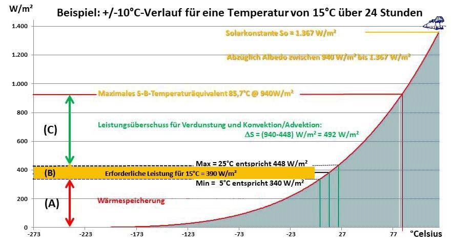
Figure 7: The relationship between temperature and specific radiative power in the Stefan-Boltzmann law. In this example, the fluctuation of +/- 10°C around a local temperature of 15°C corresponds to a change in
the specific solar radiant power of 108 W/m². The S-B relationship shown can of course also be applied accordingly to other local temperatures and their fluctuation range in the sequence of day and night.
Note: The maximum S-B temperature equivalent from solar irradiance is 85.7°C, taking into account the terrestrial albedo. The solar power range required to maintain the local temperature is ochre-coloured, below which lies the stored energy and above it the available energy for convection and evaporation.
Our Earth is a water planet, two-thirds of whose surface is covered by oceans. Both the temperature on the day side of the Earth and the temperature on its night side are supported by the temperature of the global heat storage system, which is significantly greater than 0 Kelvin. This temperature is essentially determined by the average temperature of the oceans (approx. 20°C) and does not have to be generated by the daily solar irradiation, because it is already present in this "steady" system. The heat content of the oceans is more than 4.59*10^26 joules, or 50,000 days of solar radiation, and the loss of heat at night, which is quite inconsiderable, can easily be replaced the following day. Solar radiation does not have to warm our earth from 0 Kelvin every morning, but only replace the nightly IR-radiation loss. Therefore, after the earth's surface has warmed, a lot of energy remains to replace the nightly radiation loss of the global heat storage systems from the hemispheric solar daytime irradiance alone.
In the end, it is simply correctly applied physics with which a very simple hemispheric convection model is able to represent the current state on our earth as well as its seasonal changes in a qualitatively correct way. Not much is necessary for this, an angular function for the local solar zenith angle, the solar constant and the albedo on our Earth as well as a physically correct Stefan-Boltzmann inversion for the mathematical result - done. The comparison list between my hemispheric convection model (@2PiR^2) and the conventional Factor4-
THE paradigm (@4PiR^2) available here (in German) may further illustrate the differences between these two models.