CHITRA M. KUMAR

GIS METHODS FOR SCREENING POTENTIAL ENVIRONMENTAL JUSTICE AREAS IN NEW ENGLAND

CHITRA M. KUMAR Massachusetts Institute of Technology, Department of Urban Studies + Planning

ABSTRACT

Over the past decade scholars, scientists, and community advocates have argued that minority and low-income communities have been exposed to disproportionate amounts of hazardous pollution as a result of systematic biases in policy-making and discriminatory market forces. Geographic Information Systems (GIS) is an important tool used to assist regulatory agencies in identifying these potentially vulnerable or "potential environmental justice" areas so that programmatic decision-making can incorporate EJ concerns. Yet few studies have documented or evaluated methodologies for EJ-GIS analyses utilized by public agencies. This paper explores various methodologies that approximate the relative position of communities at risk of disproportionate burden with respect to the unique character and composition of a region. Specific variables explored are race/ethnicity, poverty, and population density. For each variable a scale and threshold/reference value is determined; the possibility of establishing a ranking system is also contemplated. Finally, the importance of investigating spatial clustering and integrating variables into combined criteria is discussed. The United States Environmental Protection Agency-New England regional office was chosen as the host for this research because of its particular interest in and mandate for overseeing integration of environmental justice concerns into policy/planning activities. Based on research results, recommendations were made to EPA-New England on how to improve their demographic mapping system.

INTRODUCTION

Over the past decade scholars, scientists, and community advocates have argued that minority and low-income communities have been exposed to disproportionate amounts of hazardous pollution as a result of systematic biases in policy making and discriminatory market forces. Facing activist pressure and seeing greater evidence for "environmental injustice," President Clinton issued Executive Order 12898 in February 1994, requiring all federal agencies to examine the effects of their policy-making, regulatory, and enforcement activities with regard to environmental justice concerns. Consequently, promoting environmental justice (EJ) - defined by the Environmental Protection Agency Office of Environmental Justice as the fair treatment and meaningful involvement of all people regardless of race, color, national origin, or income with respect to the development, implementation, and enforcement of environmental laws, regulations, and policies1 - became one of the U.S. Environmental Protection Agency's top priorities.

As EJ was becoming an important concept, in 1993 EPA New England created a methodology for mapping demographic characteristics of the Region using geographic information systems (GIS). GIS allows users to spatially correlate data in order to identify "Potential Environmental Justice Areas." Since the time when the first methodology was conceived, analytic tools, data availability, and geographic mapping capabilities have greatly advanced. In response to these changes and an improved knowledge base about EJ issues, the Region's Office Directors chartered an Environmental Justice Council in 1999 with the goal of institutionalizing EJ philosophy and principles in the Region's daily program activities. The EJ Council's Mapping Workgroup, a subset of the larger Council, was tasked

To develop a computer-based Environmental Justice mapping tool covering all six New England States which is accessible to EPA New England personnel through the desktop PC and provides useful data regarding Environmental Justice issues such that Environmental Justice becomes better incorporated into the day-to-day work of the

Region (u.s. EPA, Action Plan, 2001).

The key requirements of the tool were that it allow the Region to prioritize its permitting and inspection resources and that it help the Agency move from a primarily reactive site-specific analysis that responds to complaints to a proactive region-wide programmatic decision-making tool. This paper aids EPA's mandate by exploring various methodologies to identify one that better approximates where communities at risk of disproportionate burden may be. Specifically, I will investigate different statistical methodologies for performing demographic analyses using GIS.

This research began with the problem being framed. Then, a survey of the literature and public institutions was done to identify relevant practices and state-of-the-art technology in environmental justice analysis. Next, a process was designed to develop and select an appropriate methodology. This process included meeting systematically with members of the U.S. Environmental Protection Agency New England GIS team and Mapping Workgroup of the Environmental Justice Council to discuss and compare various methods of analysis. Based on research results, recommendations were made to the EPA-New England regional office on how to improve their demographic mapping system. These recommendations will, it is hoped, be adopted by EPA-New England and introduced in a desktop GIS tool by the end of 2002.

Current Practice

Environmental Justice Screening in the Federal Government

Most academic studies of environmental justice deal with "proving" or "disproving" the existence of inequities based on race and class and, with the aid of GIS, identifying appropriate indicators that predict such a

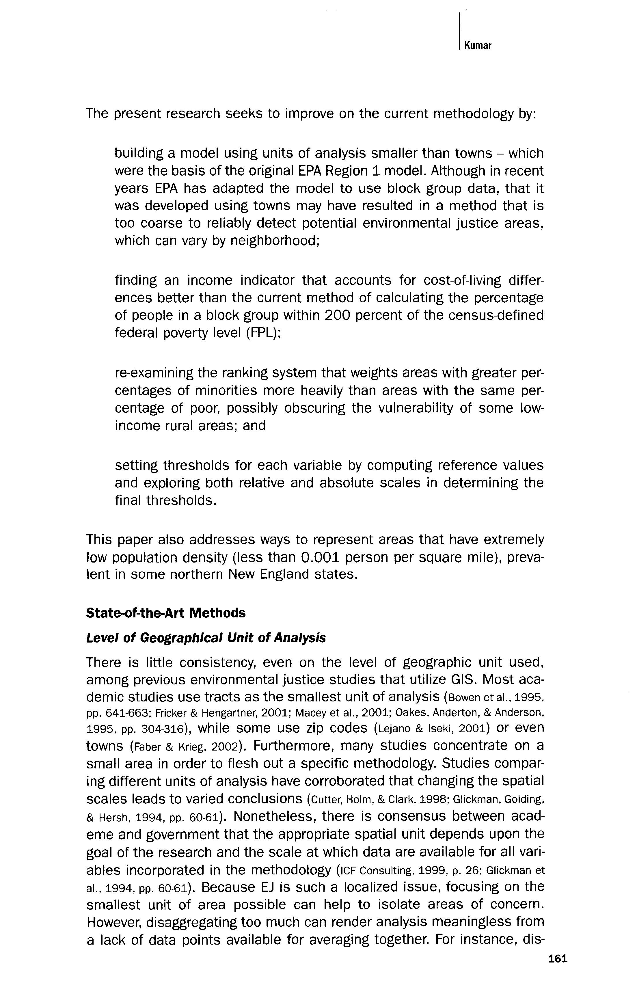
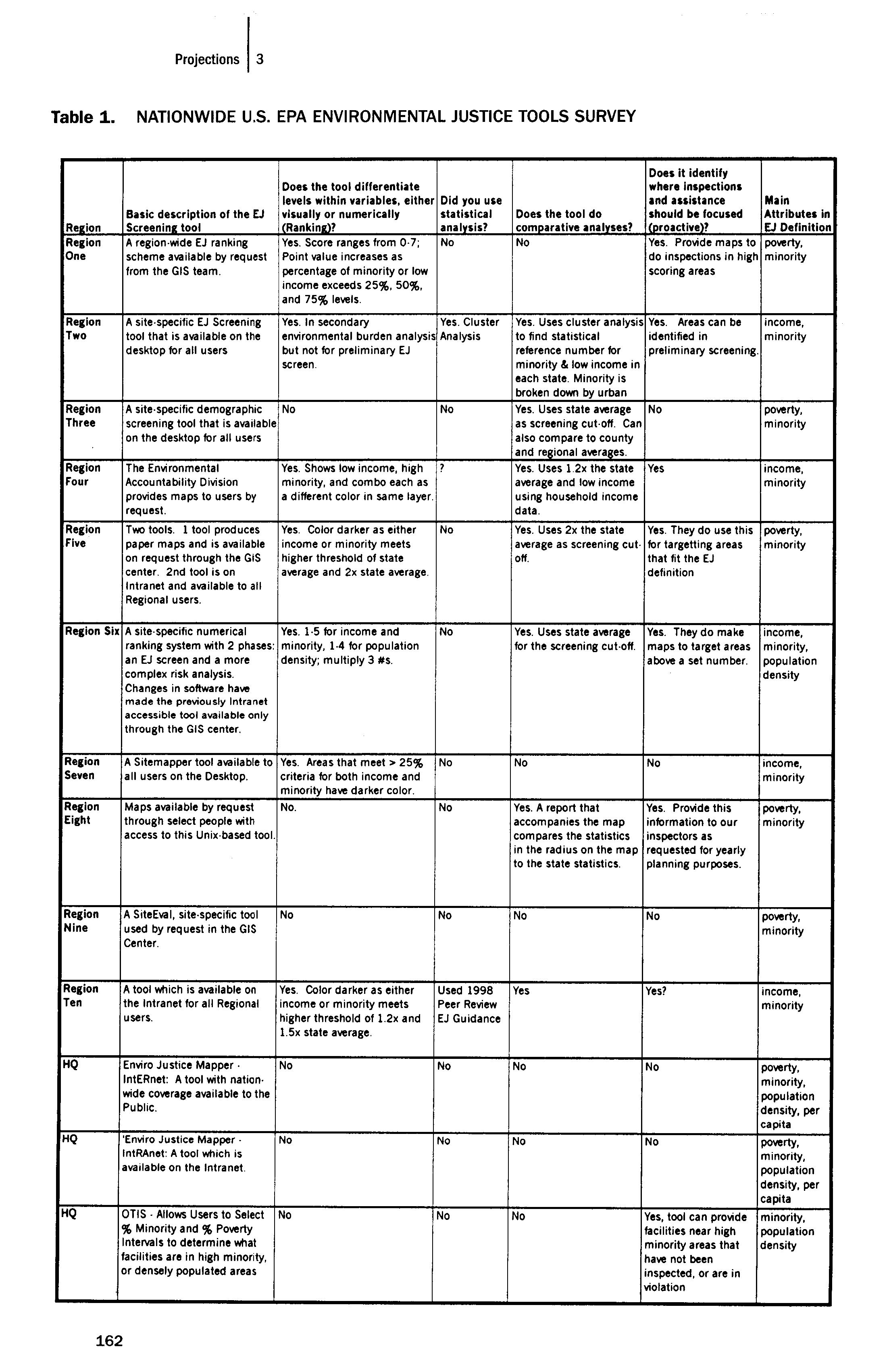
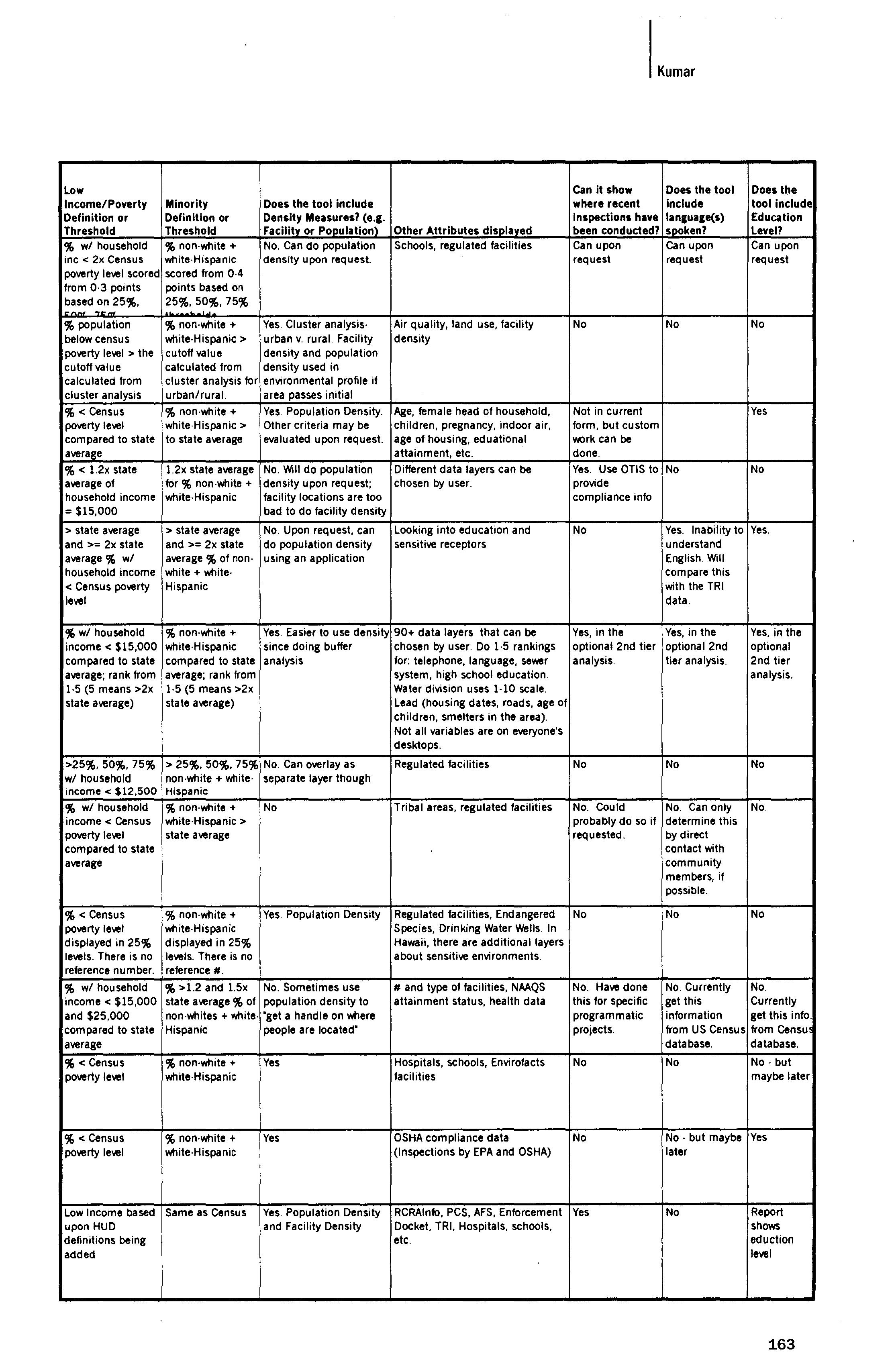
relationship (Bullard. 1983; Faber & Krieg. 2002; Fricker & Hengartner. 2001; Glickman. 1995; Lejano & Iseki. 2001; Nabalamba & Warriner. 1998; United Church of Christ [UCCl. 1987). In contrast, public agencies attempt to utilize GIS and indicators to guide regulatory decision-making. Few studies examining public agency decision tools for environmental justice concerns have been conducted. In order to fill the gap in information on the practice of incorporating EJ concerns into a government agency, the EPA conducted and released a survey of the ten EPA regional offices and EPA Headquarters in 2001, probing into EJ screening tools used in those offices. This landmark survey was among the first to report on GIS screening methods used in the agency primarily responsible for overseeing environmental justice affairs (Kumar. 2001, p. 14). The 2001 survey found that EPA does not use sophisticated statistical models to identify potential environmental justice areas, but instead simple and easy to understand spatial screens. More advanced environmental models may be used on a program-specific or case-specific basis but are not instituted agency-wide or even regionwide. The most relevant information from the survey is displayed in Table 1.

EPA-New England's Methodology

EPA Region 1 has a regional screening methodology and EJ ranking scheme that ranks and categorizes census block group percentages of minority and low-income people in categories of 25 percent and assigns a point scale with each consecutive category receiving one point higher; values are not compared to those of any other geographic unit (e.g., county or state). Map 1, "Potential Environmental Justice Areas in New England," and Map 2, "Potential Environmental Justice Areas Around Boston, MA," portray the current methodology.

The present research seeks to improve on the current methodology by:

building a model using units of analysis smaller than towns - which were the basis ofthe original EPA Region 1 model. Although in recent years EPA has adapted the model to use block group data, that it was developed using towns may have resulted in a method that is too coarse to reliably detect potential environmental justice areas, which can vary by neighborhood;

finding an income indicator that accounts for cost-of-living differences better than the current method of calculating the percentage of people in a block group within 200 percent of the census-defined federal poverty level (FPL);

re-examining the ranking system that weights areas with greater percentages of minorities more heavily than areas with the same percentage of poor, possibly obscuring the vulnerability of some lowincome rural areas; and

setting thresholds for each variable by computing reference values and exploring both relative and absolute scales in determining the final thresholds.

This paper also addresses ways to represent areas that have extremely low population density (less than 0.001 person per square mile), prevalent in some northern New England states.

State-of-the-Art Methods

Level of Geographical Unit of Analysis

There is little consistency, even on the level of geographic unit used, among previous environmental justice studies that utilize GIS. Most academic studies use tracts as the smallest unit of analysis (Bowen et aI., 1995, pp. 641-663; Fricker & Hengartner, 2001; Macey et aI., 2001; Oakes, Anderton, & Anderson, 1995, pp. 304-316), while some use zip codes (Lejano & Iseki, 2001) or even towns (Faber & Krieg, 2002). Furthermore, many studies concentrate on a small area in order to flesh out a specific methodology. Studies comparing different units of analysis have corroborated that changing the spatial scales leads to varied conclusions (Cutter, Holm, & Clark,199B; Glickman, Golding, & Hersh, 1994, pp. 60-61). Nonetheless, there is consensus between academe and government that the appropriate spatial unit depends upon the goal of the research and the scale at which data are available for all variables incorporated in the methodology (ICF Consulting, 1999, p. 26; Glickman et aI., 1994, pp. 60-61). Because EJ is such a localized issue, focusing on the smallest unit of area possible can help to isolate areas of concern. However, disaggregating too much can render analysis meaningless from a lack of data pOints available for averaging together. For instance, dis-

Table 1. NATIONWIDE U.S. EPA ENVIRONMENTAL JUSTICE TOOLS SURVEY

Rer:ion Region One Basic description of the EJ Screeninr: tool A region·wide EJ ranking scheme available by request from the GIS team. Does the tool differentiate levels within variables. either Did you use visually or numerically statistical I (Rankinr:)? analysis? Yes. Score ranges from O· 7; No Point value increases as percentage of minority or low income exceeds 25%, 50%, and 75% le\lels.

Region A site·specific EJ Screening Yes. In secondary Yes. Cluster Two tool that is available on the enllironmental burden analysis Analysis desktop for all users but not for preliminary EJ screen

Region Three

Region Four

Region Five A site· specific demographic screening tool that is available on the desktop for all users No No

The Enllironmental Accountability Division provides maps to users by request. Two tools. 1 tool prod uces paper maps and is available on request through the GIS center. 2nd tool is on Intranet and available to all Regional users. Yes. Shows low income, high minority, and combo each as a different color in same layer.

Yes. Color darker as either income or minority meets higher threshold of state a\lerage and 2x state a\lerage No Does it identify where Inspections and assistance Main Does the tool do should be focused Attributes in comparative analyses? I (Jlroactiv@1? EJ Definition No Yes. Prollide maps to PO\lerty. do inspections in high minority scoring areas

Yes. Uses cluster analysis to find statistical reference number for minority & low income in each state. Minority is broken down by urban Yes. Uses state a\lerage as screening cut· off. Can also compare to county and regional a\lerages. Yes. Uses 1.2x the state a\lerage and low income using household income data. Yes. Uses 2x the state a\lerage as screening cut· off. Yes. Areas can be identified in preliminary screening.

No

Yes

Yes. They do use this for targetting areas that fit the EJ definition income. minority

P°\lerty, minority

income, minority

po\lerty, minority

income, minority, population density

income, minority

Yes. A report that Yes. Prollide this PO\lerty, accompanies the map information to our minority com pares the statistics inspectors as in the radius on the map requested for yearly to the state statistics. planning purposes.

Region Six A site·specific numerical Yes. 1·5 for income and No ranking system with 2 phases: minority, 1·4 for population an EJ screen and a more density; multiply 3 #s. complex risk analysis. Changes in software haw made the previously Intranet accessible tool available only through the GIS center.

Region A Sitemapper tool available to Yes. Areas that meet> 25% No Seven all users on the Desktop. criteria for both income and minority ha\le darker color. Region Maps available by request No. No Eight through select people with access to this Unix·based tool.

Region A SiteEval, site·specific tool Nine used by request in the GIS Center.

Region A tool which is available on Ten the Intranet for all Regional users. Yes. Uses state awrage for the screening cut·off. Yes. They do make maps to target areas abo\le a set number.

No No

No No No

Yes. Color darker as either Used 1998 income or minority meets Peer Review higher threshold of 1.2x and EJ Guidance 1.5x state a\lerage. Yes

HQ Enviro Justice Mapper· IntERnet: A tool with nation· wide cO\lerage available to the PubliC. No No No

HQ 'Enlliro Justice Mapper· IntRAnet: A tool which is available on the Intranet

HQ OTIS· Allows Users to Select % Minority and % PO\lerty Intervals to determine what facilities are in high minority, or densely populated areas No No No

No No No No

Yes? pO\lerty, minority

income, minority

pO\lerty, minority, population density, per capita poIIerty, minority, population denSity, per capita minority, population density

No

No

Yes, tool can prollide facilities near high minority areas that ha\le not been inspected, or are in violation

Low Income/Poverty Does the tool include Definition or Density Measures? (e.g. Threshold Minority Definition or Threshold Facility or Population) Other Attributes displayed % w/ household % non·white + No. Can do population Schools, regulated facilities inc < 2x Census white·Hispanic density upon request. poverty lellel scored scored from 0·4 from 0·3 points points based on based on 25%, 25%, 50%, 75%

% population % non·white + Yes. Cluster analysis· Air quality, land use, faCility below census white·Hispanic> urban v. rural. Facility density poverty lellel > the cutoff value denSity and population cutoff value calculated from density used in calculated from cluster analysis for environmental profile if cluster analysis urban/rural. area passes initial % < Census % non·white + poverty lellel white·Hispanic> compared to state to state allerage average Yes. Population Density. Other criteria may be evaluated upon request. % < 1.2x state 1.2x state allerage No. Will do population allerage of for % non·white + density upon request; household income white·Hispanic facility locations are too = $15,000 bad to do facility density Age, female head of household, children, pregnancy, indoor air, age of housing, eduational attainment, etc. Different data layers can be chosen by user. > state allerage > state average No. Upon request, can Looking into education and and >= 2x state and >= 2x state do population density sensitille receptors average % w/ average % of non· using an application household income white + white· < Census pollerty Hispanic level Can it show Does the tool where recent include inspections have language(s) been conducted? spoken? Can upon request Can upon request Does the tool include Education Level? Can upon request

No No No

Not in current form, but custom work can be done. Yes. Use OTIS to No provide compliance info Yes

No

No Yes. Inability to Yes. understand English. Will compare this with the TRI data.

Yes, in the Yes, in the optional 2nd tier optional 2nd analysiS tier analysis.

% w/ household income < $15,000 compared to state average; rank from 1·5 (5 means >2x state average)

% non·white + Yes. Easier to use density 90+ data layers that can be white·Hispanic since doing buffer chosen by user. Do 1·5 ran kings compared to state analysis for: telephone, language, sewer average; rank lrom system, high school education. 1·5 (5 means >2x Water division uses 1·10 scale. state allerage) Lead (housing dates, roads, age of children, smelters in the area). Not all variables are on elleryone's desktops. >25%, 50%, 75% > 25%, 50%, 75% No. Can overlay as Regulated facilities w/ household non·white + white· separate layer though income < $12,500 Hispanic No No Yes, in the optional 2nd tier analysis.

No

% w/ household % non·white + No income < Census white·Hispanic> poverty level state average compared to state average Tribal areas, regulated facilities No. Could No. Can only No probably do so if determine this req u ested. by direct contact with community members, if possible.

Regulated facilities, Endangered No % < Census poverty lellel displayed in 25% levels. There is no

% non·white + Yes. Population Density white·Hispanic displayed in 25% levels. There is no reference number. reference #. % w/ household % >1.2 and 1.5x No. Sometimes use income < $15,000 state allerage % of population density to and $25,000 non·whites + white· 'get a handle on where compared to state Hispanic people are located' average % < Census poverty level % < Census poverty lellel % non·white + white·Hispanic % non·white + white·Hispanic Yes Species, Drinking Water Wells. In Hawaii, there are additional layers about sensitive environments.

# and type of facilities, NAAQS attainment status, health data

Hospitals, schools, Envirofacts facilities No. Have done this for specific programmatic projects.

No No No

No. Currently No. get this Currently information get this info. from US Census from Censu database. database. No No· but maybe later

Yes OSHA compliance data No (Inspections by EPA and OSHA)

Low Income based Same as Census upon HUD definitions being added Yes. Population DenSity RCRAlnfo, PCS, AFS, Enforcement Yes and Facility Density Docket, TRI, Hospitals, schools, etc. No . but maybe Yes later

No Report shows eduction level

aggregating to the housing unit level could identify individual household or family characteristics, but would say nothing of neighborhood or community phenomena.

Variables of Interest

Many variables have been identified in the literature and are commonly used by regulatory agencies as indicators of the level of community wellbeing or potential vulnerability to environmental injustice. Two of these demographic variables are racial/ethnic minority and income, which may be measured in different ways (ucc, 1987). These indicators are consistent with the mission of the U.S. Executive Order 12898 and subsequent environmental justice policies.

Another criterion that could be highly correlated with EJ disputes and could play into resource targeting is population density (Gragg et aI., quoted

in ICF, 1999, p. 15; Anderton et aI., 1994a, quoted in ICF, 1999, pp. 26-27). Some studies use the census definition of urbanized area (UA) as a proxy for population density because it acknowledges that a minimum concentration of population is necessary to gain economies of scale, which is desirable for industries; it requires a level of infrastructure development (or builtup area) that could facilitate new development; and it represents areas where higher land value and, thus, higher cost of living might be. Moreover, for various socio-political reasons minorities tend to be concentrated in urban areas. EPA Region 2 (New York, New Jersey, Puerto Rico, and the Virgin Islands) incorporates urban and rural criteria into their methodology 2 (see Table 1). Only one other EPA region (Region 6) includes population density in its definition. Most other regions leave population density or urbanized areas as an optional layer.

The literature and EPA have identified other demographic variables that predict the existence of potential EJ areas with varying strength. These variables include: dwelling value, unemployment (Jarret et aI., 2001), rates of home ownership, tribal lands, language(s) spoken, level of education, age of housing, and age of household member.

For each issue of concern, (a) an appropriate measure or indicator and (b) a threshold, dividing the category into groups (i.e., high and low), must be chosen. Defining measures requires an understanding of the various ways to gather those data. For example, one could measure income as per capita income, household income, family income, or by using the federal poverty level (FPL).

Approaches for Setting Thresholds

Setting a threshold involves dividing a scale of variable values into high and low groups. To do this, methodologies that do not use regression or correlation analysis often subscribe to the use of "reference values," or

comparison values, computed from larger geographic areas than the study area. Several different levels of geography could be used to set this reference value: town, county, metropolitan area, state, entire New England region, or the nation. Once a level of geography is selected, one must decide whether to use an absolute scale (e.g., mean) or a relative scale (e.g., percentile or ratio) to create a cut-off. Also, the level that determines what an "extreme" value is must be decided upon. The mean or median value represents the ordinary or normal value, while a multiple of the mean or a higher percentile than the 60th would constitute a situation outside of the usual. One must also consider if there should be a minimum number or percentage of people in an area who meet certain criteria in order to be relevant for this type of analysis. For example, an area with only 2% minorities may need a different type of screen to establish a case of disproportionate impact requiring regulatory action.

Ranking System

Establishing a ranking or scoring system can provide another way for regions to prioritize scarce resources by understanding the extent to which potential EJ communities are concentrated in particular areas. Seven of the ten EPA regions have established thresholds (statistical reference numbers) with which to compare low income and minority percentages, usually based on proportions of the state population. Areas that meet the threshold are considered potential EJ areas. Two of ten regions (Regions 1 and 6) go one step further by assigning numerical values, or scores, based on established cut-off levels of low- income and minority population. See Table 1 for other ways in which ranking systems have been used around the nation. Some regions have chosen deliberately not to make this capability explicit in their demographic tool because they feel that scores can be misleading, given data accuracy limitations. In addition, some regions worry that scoring can prompt users to focus solely on demographic criteria at the expense of environmental burden analysis. The most valuable information for decision-makers, however, is the relationship between the two.

METHODOLOGY

My research began with a thorough review of literature about the sociopolitical phenomena that lead to the inequitable distribution of environmental risk. I then researched current practice of measuring environmental justice in academic and agency contexts. I also took into account the general demographic characteristics of New England's states and became acquainted with data that are available for this type of research. As the federal body with a clear mandate to oversee integration of environmental justice in regulation. EPA was the best host for my research. As a result of U.S. EPA New England's interest in my work, I was granted unlimited access to their on-site resources at their office in Boston,

Massachusetts. I had regular meetings with the EPA New England EJ Council's Mapping Workgroup, which consisted of eight staff members from various EPA New England offices and programs. The Workgroup gave input on several subjects pertinent to developing the methodology.

This research seeks to build on the current practice of EJ screening. Maps were created for one northern and one southern New England state. Of the three sparsely populated, mostly rural northern states Maine, New Hampshire, and Vermont -- Maine was chosen. Massachusetts was chosen from the three southern states -Connecticut, Massachusetts, and Rhode Island - to represent the more densely populated and urbanized states. Many combinations of geographic units of analysis and state approaches were tested; and the top few choices were presented to the Mapping Workgroup for input and discussion. Finally, a recommendation for the methodology, guided by the evaluation criteria outlined below and background research, was proposed.

The evaluation criteria used to narrow the list of possible methodology options were:

1. Congruity between variables - the method applied to one variable should not conflict with the approach applied to other variables. (This is a greater consideration when applying a ranking system to the model.)

2. Transferability - other regions should be able to adopt it.

3. Simplicity - it should be fairly easily explained to and comprehended by non-technical staff.

4. Equity among the six New England states - it should be politically feasible, not causing contention between state governments.

5. Practicality - the analysis has to be restrictive enough to give EPA program staff confidence that the tool identifies communities with a high likelihood of being most impacted.

Criteria 3, 4, and 5 were considered to be of greater importance than 1 and 2. In addition, each methodology considered was assumed to be both a) statistically sound and b) verifiable on the ground, meaning that the predicted results match actual demographic profiles of community members.

1983, meters) data for the entire region were available on-site at the U.S. EPA New England office.

RESULTS

Level of Geographical Unit of Analysis

Many methods of analysis used by academic studies cannot be replicated for an entire region because of computational intensity or lack of data availability, and thus are not appropriate for EPA New England's use. One of the reasons for variations in level of geography used in the literature is scope of the analysis. Larger area coverage, like national or subnational, is more suited to using larger units of analysis to prevent the number of records the GIS has to handle from becoming unwieldy. Smaller study areas (e.g., region, state, town) can afford to use the smallest unit of analysis available, which is likely to be census block or block groups. Neighborhood analysis can be even further refined. For the purposes of this article, focused on New England, block groups were the smallest units for which data of interest were available and thus were adopted as the unit of analysis. According to the 2001 Survey of EPA GIS tools (Table 1), all EPA regions use block groups as the unit of analysis, supporting this decision.

Spatial Units Used for the Reference Value

There are several considerations when choosing the spatial unit for the reference value. The unit should either represent a relatively homogeneous market or a political area that has political power to effect change in the event that disproportionate burden is found. Of the options considered for developing a reference value - county, metropolitan area, state, entire New England region, or nation -a few were ruled out from the start. Counties' lack of political clout to influence well-being or vulnerability issues in New England led the Mapping Workgroup to discount them as a standard unit of analysis. However, counties are often used to characterize cost of living, since neighborhoods are too fine a scale (e.g., conSidering commuting patterns) and states, or even metropolitan areas, can be too coarse. Therefore, a county-based cost of living index would be acceptable.

Metropolitan area was not considered as a unit of analysis because, as explained later in this section, indices of how to adjust thresholds or definitions in metropolitan areas relative to rural areas were not found. Furthermore, just as with counties, metropolitan areas generally do not have political power, except when their municipalities coordinate their authority. An example of when an agency might use metropolitan area boundaries as a reference value is when Metropolitan Planning Organizations, being regional planning entities, limit their analyses to the

area that they have jurisdiction over (MORPC, <http://www.fhwa.dot.gov/environmentjejustice/case/morpc.pdf>). Based on these factors, the Mapping Workgroup suggests that this be left for future exploration and not be incorporated into this version of the methodology. The remaining three geographic areas - state, New England region, and nation - were evaluated for each variable included in the screen.

Defining Variables of Interest

In order to maintain data consistency, it is important to gather data for the entire region from one source, namely the federal U.S. Census Bureau. Deciding on a definition for race/ethnicity is relatively straightforward. The racial or ethnic groups that constitute "minority" are stated in the EPA environmental justice guidance documents to be all groups that are of non-white and/or white-Hispanic origin (u.s. EPA, Draft National

Guidance for Conducting EJ Analyses, 1998; U.S. EPA, Working Draft: Guide to Assessing and Addressing Allegations of Environmental Injustice, 2001). All EPA regions, Headquarters and most other agencies follow this convention using the 1990 census data. This method is careful not to double-count any groups, which can be a problem if the data are not well understood.3 Seeing no reason to contradict the EPA definition of "minority," this study adopts that common definition. The census fields used are: African American, Asian and Pacific American, American Indian, Eskimo, Aleut, all those of Hispanic origin, and Other non-white persons. This definition will change with the use of the 2000 Census data, since the latest survey allowed people to identify themselves under multiple race/ethnicity categories. Once 2000 census data are integrated into the GIS, the minority definition should include all people who report themselves as being in at least one of the non-white or Hispanic categories.

Defining "low-income" is a more challenging task, without consistent guidance from other organizations or agencies. There are three primary issues with identifying low-income communities. First, one must choose an indicator that adequately reflects the amount of income to an individual, family, or household. Second, the cut-off value that divides lowincome from non-low-income must be decided. Third, one must choose what concentration, or percentage, of the population in an area must be low-income in order to merit attention from an agency's programmatic standpoint. The first two issues are discussed in this section, and the third in the following section.

The challenge with defining an appropriate measure for wellbeing/income is to account for geographic differentiation in cost of living. To date, there is only one known data set of household income limits that is geographically specific and available for the entire U.S. (Hall, 1997). This special tabulation by HUD and the Census Bureau, Qualified Census Tracts (QCTs), was found to be unacceptably restrictive for EPA's use, identifying far fewer areas than the current system.4 However, QCTs

were overlaid onto the final low-income methodology to verify its accuracy.

Other measures have drawbacks that will have to be compensated for by estimation. For example, the federal poverty level (FPL) accounts for difference in income based on household size, but not geography. Alternatively, whereas median (or percentage of median) household income can be varied by geography, it is not specific to household size due to limitations in the way census data are aggregated and reported. In addition, poverty level, based on an algorithm calculated at the national level, has been criticized for being too low or otherwise inappropriate across the board (Bernstein, 2001; Boushey, 2001). It is even more questionable when dealing with regions (especially ones with many large urban areas) where the cost of living is higher than the national average. Meanwhile, using household income often inflates the percentage of households that qualify as low-income.

Although the FPL is better than other methods at accounting for changing needs based on household size, through this research it has become clear that the FPL is too low to be used on its own, especially for communities in southern New England states. Instead, 200% of the FPL is recommended as the cut-off for income.5 One study by the Economic Policy Institute (Hardships in America) supports this value as a reasonable proxy for calculating geographically specific low-income indices (Boushey et aI., 2001, p. 4). Moreover, many states use multiples of the FPL as income limits for assistance programs, several using values even greater than 200%.6 Interestingly, EPA New England's EJ methodology uses 200% of the FPL as the low-income definition. In the absence of data indicating differentials in cost of living between urban and rural areas and states, there is no basis for adjusting the multiple of the poverty level to suit state or metropolitan area characteristics. Therefore, this paper recommends that 200% of the FPL be maintained as the lowincome definition and cut-off, applied evenly throughout the region.

Population density is an additional indicator that EPA New England considered for the tool. In environmental justice analyses, population density is generally computed as the number of people per unit area (e.g., people per square mile) (Gragg et aI., 1996; ICF Consulting, 1999). This variable gives a picture of how concentrated or dispersed certain populations are. For targeting purposes, population density can be used to achieve two goals. First, it can draw attention to areas where EPA would garner the "greatest bang for the buck." Second, it can help distinguish areas with extremely low population counts so that users can decide whether or not to exclude them from the analysis.

Setting Thresholds for Key Variables Minority

In choosing a threshold for minority percentage many options were considered. Options included state, regional, or national reference values and whether to incorporate separate urban and rural thresholds. In addition, one could use an absolute scale (e.g., mean) or a relative scale (e.g., percentile). Based on discussions with EPA staff, the following promising methods for dividing the scale into high and low groups were explored:

1. Static Percent: Picking one threshold for the region and applying it consistently (e.g., 30% or 50%). This method indicates an acceptance that there is some minimum concentration of minorities, independent of spatial distribution, that constitutes an area of concern.

2. Regional or National Mean: Apply the national or regional average percentage of minorities to the entire region; acts much like a static percent. The state mean, although used by many sources, including EPA Regions 3 and 6 and Scorecard ("Environmental Justice Report Descriptions"), does not signify an extreme level of minority concentration, but rather the normal situation.

3. Factor of the Mean: Multiplying mean percentage for block groups in state or region by some factor (e.g., 1.5 or 2). This method, used by two EPA regions7 , attempts to identify areas that are extraordinarily situated, as opposed to the mean, which identifies the norm in a specified area.

4. Percentile: Sets a threshold where it is necessary to have a set percent of block groups above it (e.g., 80th percentile would have 20% of block groups above the threshold). Choosing a percentile cutoff may seem subjective.

5. Dual Criteria: Uses a combination of the above options. This method is useful only in creating state-based thresholds and is helpful in that it relaxes the range of differences between state thresholds, which is a particular concern for New England since northern states' and southern states' demographics greatly differ.

After testing several different methods, the Mapping Subcommittee chose a threshold based on the evaluation criteria laid out earlier (Congruity, Transferability, Simplicity, Equity, and Practicality). Percentile regionally was selected because Workgroup members believed that the regional approach eliminated perceived bias between states and represented the most extreme cases, whereas any method using averages

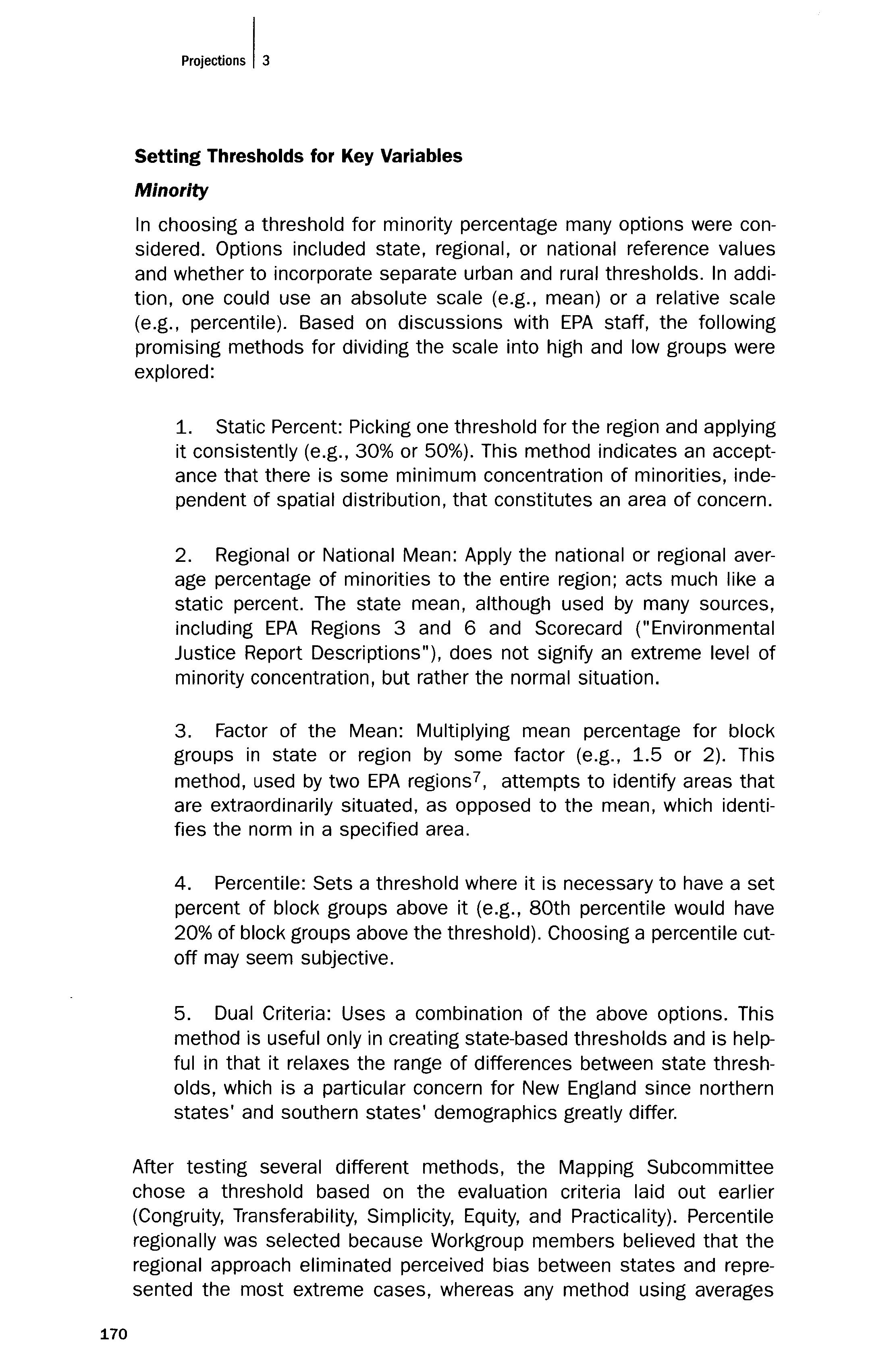
Figure 1. DECISION TREE FOR SETIING THE MINORITY THRESHOLD

Decide

Area

518/02

Figure 2 DECISION TREE FOR SETTING THE INCOME THRESHOLD

represented a contrived threshold imposed on an area. Although there is precedent for the use of state-based reference values, the group felt that state socio-political factors were not strong enough determinants of variation in distribution of minority populations to justify separate thresholds for each state. To further support the choice of method, we recalled that EPA is a regional office, interested in servicing areas in need irrespective of geographic distribution - though the office does keep spatial equity in mind - and that funds and resources are distributed accordingly.

In choosing the percentile approach, various levels were examined. For the tool to be practical, it was decided that the percentile level should be sufficiently restrictive. The 85th percentile resulted in a regional break of 18.3% with block groups having higher than the break considered as "potential environmental justice areas." This break is somewhat less restrictive than the current threshold of 25% but is close to other values the Mapping Workgroup was considering, such as the national average (24.6%) and twice the regional average (21.1%). The chosen percentile means that the top 15 percent of block groups with highest minority percentages will be included. It assures that unusually high-percentage minority populations will be identified, which is representative of communities most potentially vulnerable to "double jeopardy" (sociological and environmental health risks compounded) or disproportionate burden.

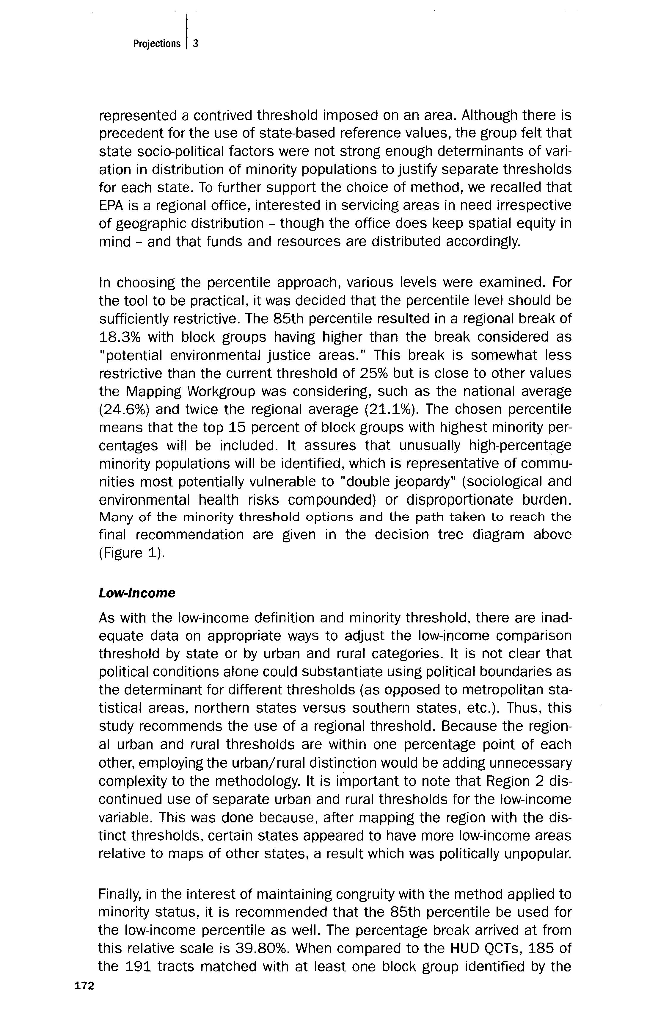
Many of the minority threshold options and the path taken to reach the final recommendation are given in the decision tree diagram above (Figure 1).

Low-Income

As with the low-income definition and minority threshold, there are inadequate data on appropriate ways to adjust the low-income comparison threshold by state or by urban and rural categories. It is not clear that political conditions alone could substantiate using political boundaries as the determinant for different thresholds (as opposed to metropolitan statistical areas, northern states versus southern states, etc.). Thus, this study recommends the use of a regional threshold. Because the regional urban and rural thresholds are within one percentage point of each other, employing the urban/rural distinction would be adding unnecessary complexity to the methodology. It is important to note that Region 2 discontinued use of separate urban and rural thresholds for the low-income variable. This was done because, after mapping the region with the distinct thresholds, certain states appeared to have more low-income areas relative to maps of other states, a result which was politically unpopular.

Finally, in the interest of maintaining congruity with the method applied to minority status, it is recommended that the 85th percentile be used for the low-income percentile as well. The percentage break arrived at from this relative scale is 39.80%. When compared to the HUD QCTs, 185 of the 191 tracts matched with at least one block group identified by the

Map 1. POTENTIAL ENVIRONMENTAL JUSTICE AREAS IN NEW ENGLAND REGION

Zero

One

Two

Three

Four

Five

Six

Seven

Unpopulated

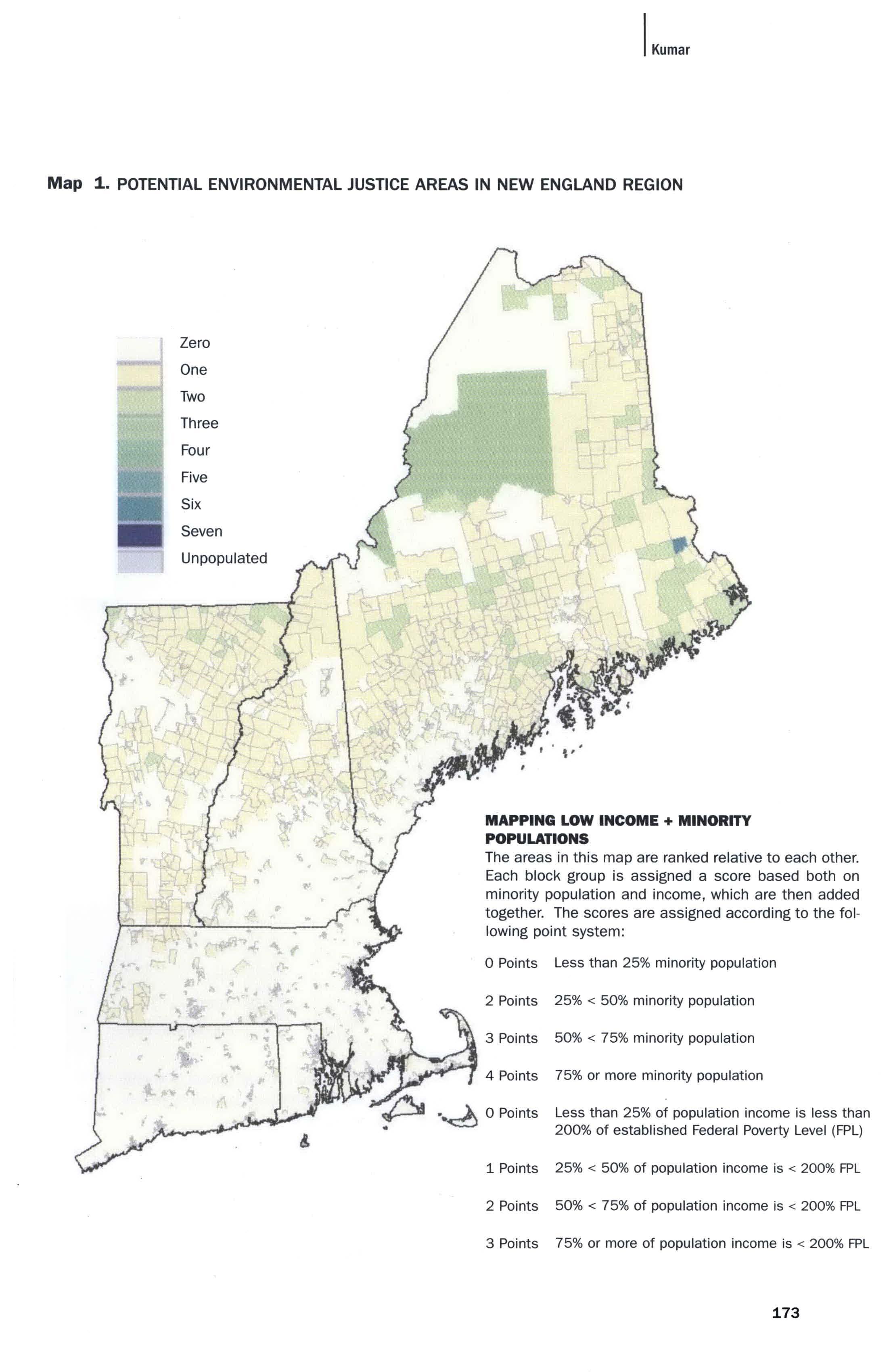
MAPPING LOW INCOME + MINORITY POPULATIONS

The areas in this map are ranked relative to each other. Each block group is assigned a score based both on minority population and income, which are then added together. The scores are assigned according to the following point system:

oPoints Less than 25% minority population

2 Points 25% < 50% minority population

50% < 75% minority population

75% or more minority population

... o Points Less than 25% of population income is less than 200% of established Federal Poverty Level (FPL)

1 Points

2 Points

3 Points 25% < 50% of population income is < 200% FPL

50% < 75% of population income is < 200% FPL

75% or more of population income is < 200% FPL

Map 2. , POTENTIAL ENVIRONMENTAL JUSTICE AREAS AROUND BOSTON, MA

I

II/on

One Two Three Four Five Six Seven Population Area

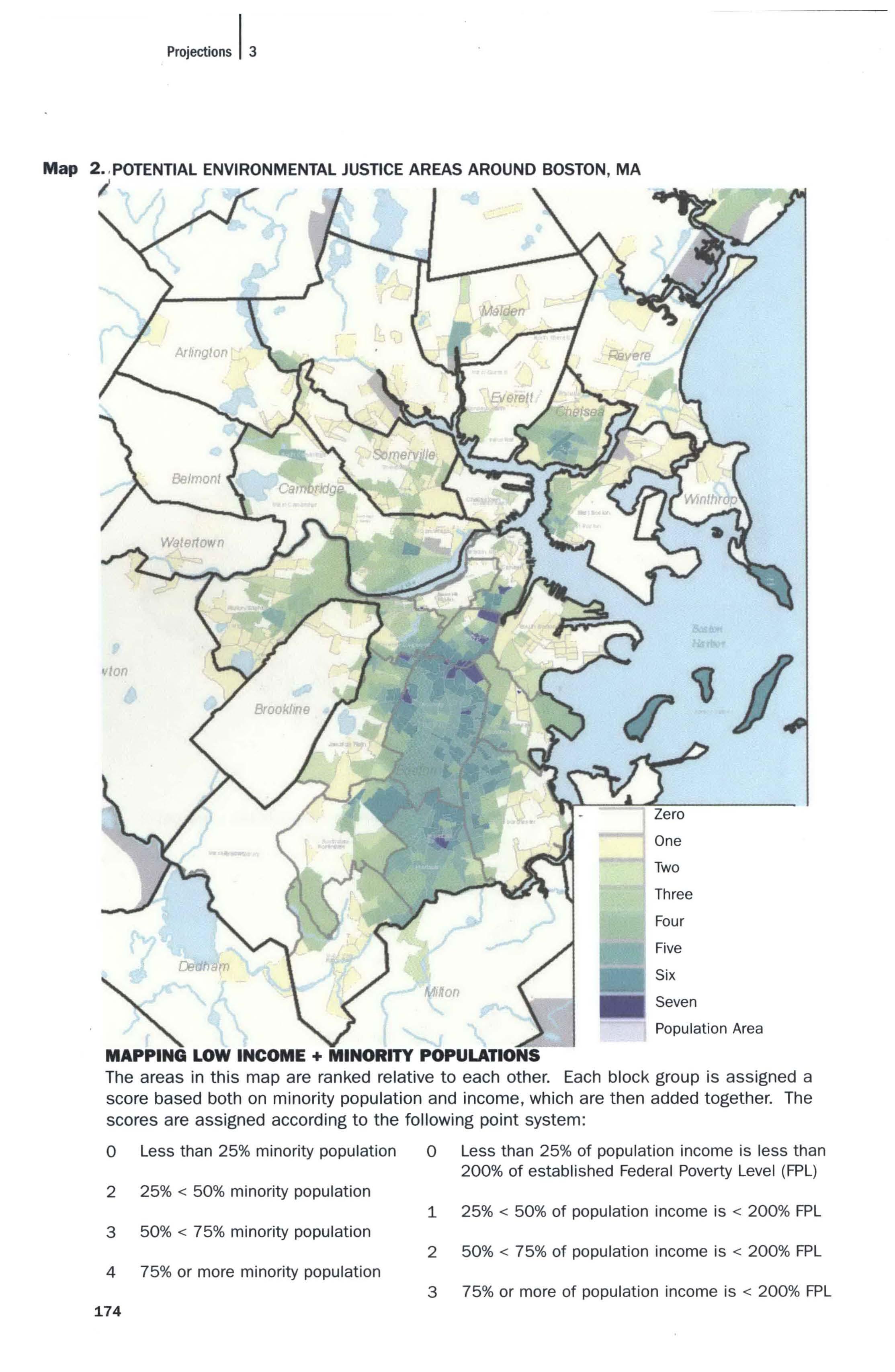
MAPPING LOW INCOME + MINORITY POPULATIONS

The areas in this map are ranked relative to each other. Each block group is assigned a score based both on minority population and income, which are then added together. The scores are assigned according to the following point system: 0 Less than 25% minority population 0 Less than 25% of population income is less than 200% of established Federal Poverty Level (FPL)

2 25% < 50% minority population

1 25% < 50% of population income is < 200% FPL

3 50% < 75% minority population

2 50% < 75% of population income is < 200% FPL

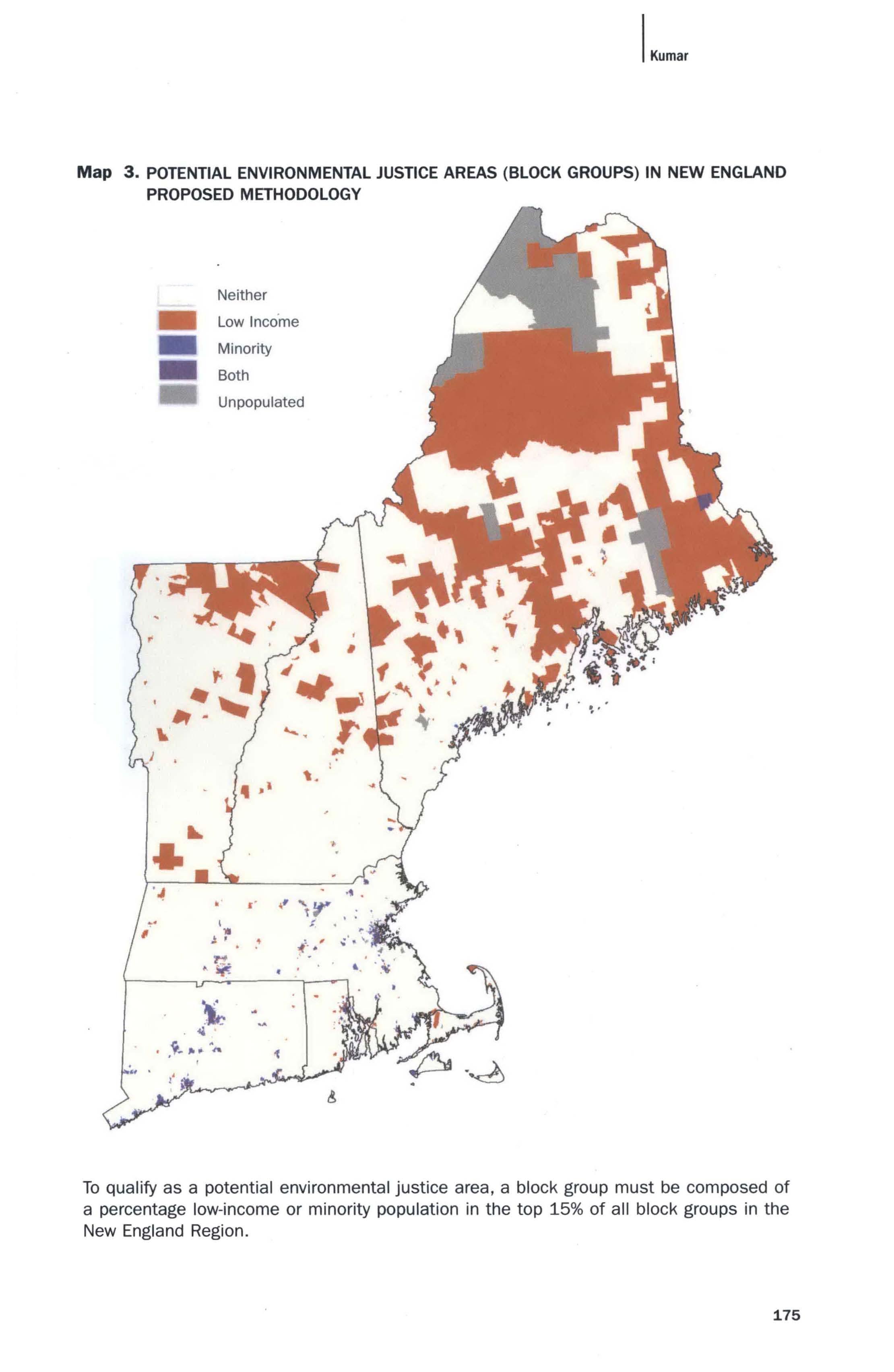
Map 3. POTENTIAL ENVIRONMENTAL JUSTICE AREAS (BLOCK GROUPS) IN NEW ENGLAND PROPOSED METHODOLOGY

Neither Low Inco'me

Minority Both Unpopulated

To qualify as a potential environmental justice area, a block group must be composed of a percentage low-income or minority population in the top 15% of all block groups in the New England Region.

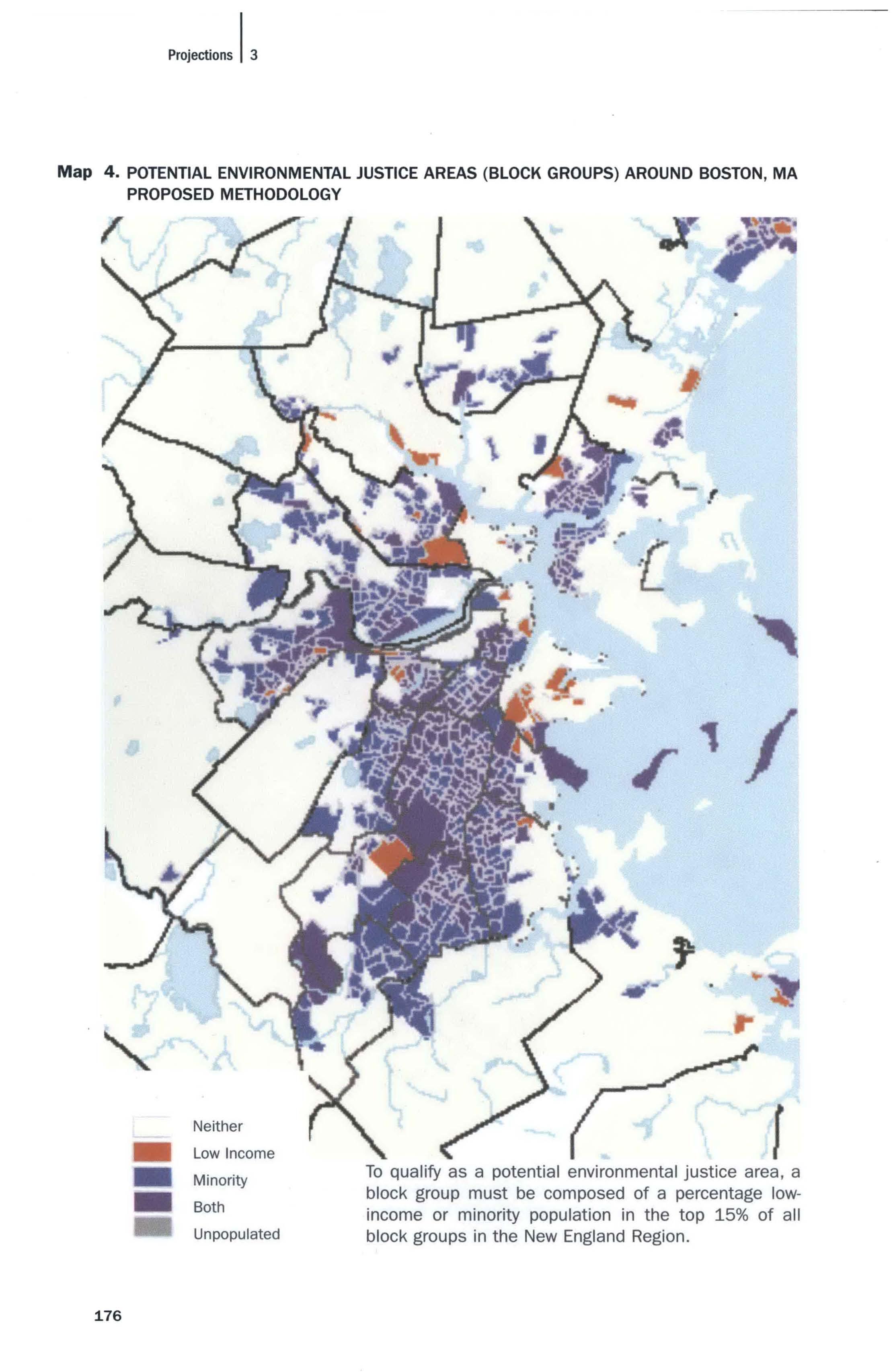
Map 4. POTENTIAL ENVIRONMENTAL JUSTICE AREAS (BLOCK GROUPS) AROUND BOSTON, MA PROPOSED METHODOLOGY

Minority 80th

Unpopulated To qualify as a potential environmental justice area, a block group must be composed of a percentage I owincome or minority population in the top 15% of all block groups in the New England Region.

proposed methodology. This nearly 97% congruence rate is seen as a strong indicator of the validity of the new methodology. The six non-conforming tracts were all in Massachusetts or Connecticut and were adjacent to block groups that qualified under the proposed methodology. Four of the six tracts were in metropolitan areas. One possible reason that six tracts did not overlap with the proposed methodology is that high cost of living in those areas caused HUD tracts to qualify but was not accounted for by the non-geographically-specific FPL used in the proposed methodology. Another reason could be that HUD's special tabulation uses annually reported data, and these six areas represent recently developed areas not captured in the 1990 census.

A simplified version of the decision process through which the recommendation for the income threshold was reached is shown in Figure 2.

Population Density

Population density can be incorporated into the tool either as part of the definition of a potential environmental justice area or as an overlay to the preliminary screen. Either method of utilizing population density can help targeting efforts. If it is made part of the definition, EPA implies that population density is an intrinsic part of the decision-making process. On the other hand, keeping population density as a removable overlay gives users the flexibility to decide the importance of density with respect to other layers based on their programmatic functions and goals.

There are two significant reasons not to include population density in the preliminary screen. First, urban areas dominate population density maps and can attract attention away from equally deserving rural areas or show a bias toward the more populous southern states. Second, while race and income are explicitly mentioned in the Regional Environmental Justice Policy, population density (or even population size) is not (u.s. EPA New England, 2001). Therefore, population density should be included in the GIS tool as an overlay, separate from the basic potential environmental justice definition of minority and income status. Since population density was deemed a secondary consideration, the specifics of threshold choice were not explored fully before publication of this research. However, thresholds should be set before the release of the GIS application.

When discussing population density it is important to note that the land area of the unit of analysis, block group, varies drastically throughout the Region based on household concentration. In densely populated areas, a small increase in block group size could easily change an area's potential EJ status. Also, a community could encompass several block groups, making it necessary to investigate the spatial distribution of block groups in relation to neighboring block groups. In other words, block groups can-

not and should not be treated as isolated individual entities but, rather, the existence of clusters of potential EJ block groups should also be identified. Clustering in low-density areas could also suggest an EJ concern depending on the programmatic issue at hand. Therefore, in defining community vulnerability low-density and high-density areas would have to be considered by distinct criteria that accounted for the role of both the size and density of clusters.

Creating a method that evaluates clustering could satisfy the need to assess population distribution over land area and help evaluate larger units of analysis. Although this concept was not discussed by the EPA Region 1 Mapping Workgroup for incorporation into the 2002 version of the EJ-GIS application, it does merit investigation for future versions of the GIS tool.

In the absence of a separate screening method for exceedingly low population density areas that skew calculations, as in northern New England, some studies exclude such areas from analyses. For instance, in a Logan Airport study, areas with fewer than 10 persons per square mile were displayed as unpopulated (Aguilar & Haracz, 2002). To compensate for this problem, the population density overlay should demarcate areas that have extremely low population densities (i.e., less than 1 person/square mile) as well as the high end of most densely populated block groups.

Ranking

Although a ranking would provide more information for users, allowing them more flexibility in their analysis, the Mapping Workgroup felt that a ranking or scoring system implied a level of precision that is not available. In addition, it was decided that without a ranking system, users would be more likely to critically examine the results of the EJ maps and might look into other overlays that could help prioritize areas, rather than relying too heavily on the low-income and minority factors alone.

As a result, maps will be displayed as "one-other-both" - areas that are only minority ("one") will be distinguishable from areas that are I owincome only ("other"); and areas that are both minority and low-income will be a third variation, distinguishable from the rest. The minority variable is no longer weighted as it was in the previous Region 1 methodology since there is no consensus in the literature as to which of the minority and income variables is a better predictor of environmental justice concerns. This symbolization will be available at the 85th percentile and 95th percentile. Maps 3 and 4 show the final proposed methodology for New England and the Boston area, respectively.

deeply that researchers have had great difficulty parsing them (Maantay, 2002). This interdependence could deserve regulatory attention to aid in counterbalancing the lack of political clout or lack of general community well-being in areas that meet multiple criteria. One way to account for the association between income and race/ethnicity would be to have two thresholds for screening. The higher percentile threshold would be the value necessary to be categorized as a potential EJ community based on a single criterion (either minority or income). The lower percentile threshold would be the cutoff needed if both factors were extreme but neither was extreme enough to meet an individual criterion. For example, the 95th percentile could be the more stringent individual cutoff and the 85th percentile could be used for the lower multi-variable threshold.

DISCUSSION

The methodology recommendations laid out in this research represent extensive research and close interaction with EPA Region 1 staff. In this section, I will describe how the chosen methodology compared to the evaluation criteria and to the current EPA New England method, with regard to the perceived problems of the current system.

The proposed screening methodology meets all five evaluation criteria established by the Mapping Workgroup. Specific features that relate to the criteria are as follows:

1. Congruity between variables -thresholds for both minority and lowincome use the percentile approach at the regional scale and are set at the same levels (85th and 95th percentiles).

2. Transferability - the percentile method could easily be applied in other regions and would be reasonable even in states where the demographic composition is very different from New England. This is true because the percentile approach uses a relative scale that is less sensitive to outlying values. Moreover, the definitions for minority and low-income, race/ethnicity and 200% of the federal poverty limit, respectively, are drawn from federal databases and thus can be used by any region in the U.S. Census data are uniformly collected and computed and more easily available as compared to private or localized information sources.

3. Simplicity - the percentile approach used for thresholds is easily explained relative to other statistical techniques that involve interpolation or estimation algorithms. In addition, as explained in 2, the definitions for minority and low-income, based on national sources, are relatively well known and therefore easy to explain or understand.

4. Equitable to states - Arguably, regional scale analysis eliminates some bias between states and focuses on the scale of authority of EPA New England, a regional office.

5. Practical - The proposed methodology identifies approximately 50% fewer block groups than the current system, which represents a sufficiently restrictive level to prioritize scarce resources based on EJ concerns.

Of the initial goals for improvement upon the current methodology, some of the concerns are better addressed by the proposed approach than others. First, the proposed method uses block groups as the unit of analysis, just as EPA Region 1 has been doing in recent years. However, the recommended approach was developed to be sensitive to the finer-grain analysis of block groups, which is not the case in the original 1993 EPA method that used towns. Block group scale analysis seems to be very important, judging by a survey of areas qualifying under the proposed methodology. One can see that towns are not homogeneous in minority and/or low-income composition. For example, the town of Boston is extremely diverse, and of Boston's many neighborhoods not one is uniformly potential EJ or non-potential EJ. Each neighborhood has pockets of each status area, and conversely, more affluent and predominantly white towns such as Brookline have some block groups that meet the screening criteria.

In addition, the proposed spatial clustering analysis can compensate for the inherent dependence on census-defined units of analysis. From a brief scan of the results, there is no clear, universal pattern of clustering of areas identified by the proposed methodology. Some block group clusters exist in southern New England states' urban areas, especially of minority populations. This could be true because minorities tend to reside in homogeneous communities that often expand over time, attracting more people of the same races/ethnicities. It could also be a sign of "ghettoization" or marginalization of minorities, requiring government attention. Clusters of low-income block groups are in both urban and rural areas and show up most glaringly in northern Vermont and much of Maine. This is most probably indicative of problems of rural poor, or alternatively, of unconventional lifestyles that depend less on cash income. These varied results of block group clustering prompt greater investigation as to the driving forces behind such patterns, the conclusions of which could lead to very different policy implications.

Another improvement goal was to be able to adjust the low-income definition based on cost of living differences across New England. Unfortunately, because of data availability and resource constraints, such a measure was not established for this paper. However, a defensible proxy was found in the 200% of the FPL together with the percentile

threshold. Finally, the proposed method replaces the ranking system that weights the minority variable over the income criteria with a simple display that shows which of the variables an area qualifies for, or if both criteria are met. The display will be at both the 85th and 95th percentiles, so that users can choose if and how to weight either individual criterion versus the combination of the two. Nonetheless, it is suggested that areas that qualify by multiple criteria be held to lower percentile levels because the cumulative effects of those combined factors may indicate levels of community vulnerability similar to higher percentile levels of any one criterion.

The proposed method is effective at identifying areas that could most benefit from Agency attention because of their probable lack of internal resources to protect from environmental hazards. EPA can choose to administer its authority by limiting approval of new facility permits, increasing the rate of facility inspections, increasing community outreach on issues of lead abatement, asthma, brownfields redevelopment, and much more.

Future Studies

Further research needs before subsequent versions of the GIS tool are released include a better system to account for cost of living differences across the region; an improved understanding of ways in which population density and urbanization impact environmental justice issues (especially calculating the extent and strength of spatial clusters); and ways to weight areas that meet multiple criteria. One step to assure accuracy is field-testing borderline cases (block groups identified in some tested methodologies, but not others). Doing further research on the ground, rather than solely from census data, would provide a deeper understanding of those borderline communities. The methodology that best locates areas with the greatest potential for facing environmental injustice should be selected.

Finally, to get a true picture of environmental justice, one must be able to characterize both the demographics of an area and the environmental burden. The proposed method includes demographic factors only, leaving environmental impact analysis up to each regulatory program. In the future, EPA may consider ways of standardizing this process through a secondary environmental screen, such as Region 2's Environmental Load Profile.

Conclusion

Although many other systems may be defensible, a year of detailed research suggests that the approach laid out here is the most appropriate for the specific character and composition of New England and the regulatory needs of EPA Region 1. The proposed methodology is believed

to be a defensible indicator of areas that are most vulnerable to adverse health effects from environmental pollutants because of pre-existing negative socio-economic conditions. These areas may also have less political power and/or resources to maneuver through a complex capitalist, democratic system that arguably created the need for an environmental justice movement in the first place. Furthermore, communities identified through the screening tool may benefit most from special attention from regulatory bodies that are interested in equitably distributing their resources and reversing harmful trends.

Nevertheless, as with any decision-making tool, the user must exercise good judgment and maintain keen awareness of factors important to addressing EJ concerns, yet omitted from the tool. Explicit guidance on the limitations of GIS analysis is essential. Furthermore, mandatory EJ awareness training, as is being implemented in Region 1, is a key antecedent to institutionalization of a screening tool. Awareness training can elevate staff members' interest in EJ mapping and their ability to view results critically.

It is hoped that these recommendations will be the basis of a GIS tool to be introduced to EPA New England staff by the end of 2002.

REFERENCES

Aguilar, J., & Haracz, J. (2001,9-13 July). Environmental justice: Visualization and analyses with GIS to facilitate informed decisions. ESRI User Conference Proceedings, ESRI Library. Retrieved April 22,2002, from http://www.esri.com/library/userconf/proc01/professional/papers/pap523/p523.htm

Anderton, D. L., Anderson, A.B., Oakes, J.M., & Fraser, M.R. (1994a). Environmental equity: The demographics of dumping. Demography, 31(2), 229-248.

-. (1994b). Issues in metropolitan hazardous waste facilities: "Environmental equity." Evaluation Review, 18(2), 123-140.

Baker, A., & Cruz, G. (1998). A study on environmental equity in Albuquerque, New Mexico: Executive summary. In GIS in Public Health 3rd National Conference Proceedings (pp. 3-7). San Diego. Retrieved from http://www.atsdr.cdc.gov/gis/conference98/proceedings/proceedings.html

Been, V. (1994). Locally undesirable land uses in minority neighborhoods: Disproportionate siting or market dynamics? Yale Law Journal, 103, 1383-1422.

Bernstein, J. (2001, June). Let the war on the poverty line commence (Working Paper Series). New York: The Foundation for Child Development.

Boushey, H. et al. (2001). Hardships in America. Washington, DC: Economic Policy Institute.

Bowen, W. M. et al. (1995). Toward environmental justice: Spatial equity in Ohio and Cleveland. Annals of the Association of American Geographers, 85, 641-663.

288.

-. (1994). Unequal protection: Environmental justice and communities of color. San Francisco: Sierra Club Books.

Catalog of Federal Domestic Assistance. (2002, February 14). 21:008: Low-income taxpayer clinics. Retrieved March 1, 2002, from http://aspe.hhs.gov/cfda/p21008.htm

Cutter, S. L. (1998). Issues in environmental justice research. GIS in Public Health 3rd National Conference Proceedings (pp. 525-531). San Diego. Retrieved July, 2001, from http://www.atsdr.cdc.gov/gis/conference98/proceedings/proceedings.html

Cutter, S. L., Holm, D., & Clark, L. (1996). The role of geographic scale in monitoring environmental justice. Risk Analysis, 16, 517-526.

Faber, D. R., & Krieg, E. J. (2002, April). Unequal exposure to ecological hazards: Environmental injustices in the Commonwealth of Massachusetts. Environmental Health Perspectives, 110, 277-288.

Foreman, D. L., Wilkins, A. A. C., & West, D. (1998). Potential risk indexing system (P-RISK Model) utilizing GIS to rank geographical areas, industrial sectors, facilities, and other areas of concern. In GIS in Public Health 3rd National Conference Proceedings (pp. 53-62). San Diego. Retrieved July, 2001, from http://www.atsdr.cdc.gov/gis/conference98/proceedings/proceedings.html

Fricker, R. D., & Hengartner, N. W. (2001). Environmental equity and the distribution -of toxic release inventory and other environmentally undesirable sites in metropolitan New York City. Environmental and Ecological Statistics, 8, 33-52.

Glickman, T. S. (1995). Evaluating environmental equity in Allegheny County. In I. K. Wernick (Ed.), Community risk profiles: A tool to improve environment and community health. New York: Rockefeller University Program for the Human Environment.

Glickman, T. S., Golding, D., & Hersh, R. (1994). GIS-based environmental equity analysis: A case study of TRI facilities in the Pittsburgh area. In W. A. Wallace & E. G. Beroggi (Eds.), Computer supported risk management (pp. 95-114). The Netherlands: Kluwer, Dordrecht.

Gragg III, R. D., et al. (1996, Fall). Location and community demographics of targeted environmental hazardous sites in Florida. Journal of Land Use & Environmental Law, 12(1), 1-25.

Hall, L. (1997, January 21). Interim DRAFT EJ issues discussion (draft internal document). Wasington, D.C.: United States Environmental Protection Agency, Office of Civil Rights.

ICF Consulting. (1999). Review of technical applications for assessment of environmental justice - Draft report (prepared for Michele Wayland, United States Environmental Protection Agency, Air Quality Trends and Analysis Group, Research Triangle Park, NC).

Jarret, M., et al. (2001). A GIS-environmental justice analysis of particulate air pollution in Hamilton, Canada. Environment and Planning A, 33, 955-973.

Kumar, C. M. (2001). Draft U.S. Environmental Protection Agency regional environmental justice mapping methodologies: Report and recommendations for EPA New England. Boston: Environmental Careers Organization.

Lee, D. (2001, October 15). Examining environmental justice using GIS. Retrieved March 22, 2002, from http://gisweb.athena.bcit.ca/students/class01-02/gisa011/litreview.html

Lejano, R. P., & Iseki, H. (2001). Environmental justice: Spatial distribution of hazardous waste treatment, storage and disposal facilities in Los Angeles. Journal of Urban Planning and Development, 127(2), 51-62. Retrieved October, 2001, from http://www.pubs.asce.org

Macey, G. P., Her, X., Reibling, E.T., & Ericson, J. (2001). An investigation of environmental racism claims: Testing environmental management approaches with a geographic information system. Environmental Management, 27, 893-907.

Mank, B. C. (2001). Proving an environmental justice case: Determining an appropriate comparison population. Virginia Environmental Law Journal, 365-430.

McMaster, R. B., Leitner, H., Sheppard, E. (1997). GIS-based environmental equity and risk assessment: Methodological problems and prospects. Cartography and Geographic Information Systems, 24(3), 172.

Maantay, J. (2002, April). Mapping environmental injustices: Pitfalls and potential of geographic information systems in assessing environmental health and equity. Environmental Health Perspectives, 110, 161-171.

Martinez, M. (2001, September 11). Statutorily mandated designation of difficult development areas and qualified census tracts for Section 42 of the Internal Revenue Code of 1986. Docket No. FR-4401-N-05. Retrieved April 1, 2002, from http://www.huduser.orgjdatasets/qctjNOTICE2002.htm

Mid-Ohio Regional Planning Commission. (2001). MPO environmental justice report, Columbus, Ohio. In Environmental justice case studies. United States Department of Transportation - Federal Highway Administration - Federal Transit Administration. Retrieved March 22, 2002, from http://www.fhwa.dot.gov/environmentjejustice/case/morpc.pdf

Morello-Frosch, R., Pastor, M., & Sadd, J. (2001). Environmental justice and Southern California's "riskscape": The distribution of air toxics exposures and health risks among diverse communities. Urban Affairs Review, 36(4), 551-578.

Nabalamba, A., & Warriner, G. K. (1998). Environmental equality: Pollution, race and SOCiOeconomic status in Michigan. Environments, 26(2), 58-75.

New Jersey Department of Human Services. (2001). Regional job access and reverse commute planning: North Jersey Transportation Planning Authority and New Jersey Workfirst Program. In Environmental justice case studies. United States Department of Transportation Federal Highway Administration - Federal Transit Administration. Retrieved March 22, 2002, from http://www.fhwa.dot.gov/environmentjejustice/case/case2.htm

Oakes, J. M., Anderton, D. L., & Anderson, A. B. (1995). Environmental inequity, industrial siting, and the structure of American cities. Challenges Facing Environmental Professionals/Public and Stakeholder Involvement, Sessions M4D, M5D, 304-316.

Pittard, S. (1999, August 31). Using a geographic information system to perform environmental justice analyses in the California Energy Commission's power plant licensing process. Sacramento: University of Southern California. Retrieved March 22, 2002, from http://www.usc.edu/deptjgeography/learngis/papers/pittard583b.htm

Public Issues Education, North Carolina State University. (2001, June.) Selected definitions related to environmental justice. Retrieved April 17, 2002, from http://www.ces.ncsu.edu/depts/agecon/PEljenvjust2.html

Scorecard from Environmental Defense. (2002). Environmental justice report descriptions. Retrieved April 21,2002, from http://www.scorecard.orgjenvreleases/ def/ eLreporCdescri ptions. htm I#hotspots

-. (2002). About Scorecard. Retrieved April 21, 2002, from http://www.scorecard.orgjaboutjabout.tcl

United Church of Christ, Commission for Racial Justice (UCC). (1987). Toxic Wastes and Race in the United States: A National Report on the Racial and Socioeconomic Characteristics of Communities with Hazardous Waste Sites. New York: United Church of Christ.

United States Department of Health and Human Services, Administration for Children and Families, Low Income Home Energy Assistance Program (LiHEAP), Division of Energy Assistance/OCS/ ACF. (2002, 14 February). Eligibility guidelines. Retrieved March 1, 2002, from http://www.acf.dhhs.gov/programs/liheap/eligible.htm

United States Department of Housing and Urban Development. (2001, 11 December). Qualified census tracts and difficult development areas. PD&R Data Sets. Retrieved April 1, 2002, from http://www.huduser.orgfdatasets/qct.html

United States Department of Transportation. (2002,9 April). The facts: Environmental justice. Retrieved April 29, 2002, from http://www.fhwa.dot.gov/environmentjejustice/facts/index.html

United States Environmental Protection Agency. (1993). Equity in environmental health: Research issues and needs. Toxicology and Industrial Health, 9(5).

United States Environmental. Protection Agency. (1998). Draft national guidance for conducting EJ analyses. Washington, DC: Office of Environmental Justice.

United States Environmental Protection Agency. (2001). Working draft: Guide to assessing and addressing allegations of environmental injustice. Washington, DC: Office of Environmental Justice.

United States Environmental Protection Agency New England. (2001, 16 August). EPA New England environmental justice action plan for Fiscal Years 2001 and 2002.

United States Environmental Protection Agency, Office of Enforcement and Compliance Assurance. (2002, 24 January). Environmental justice. Retrieved April 22, 2002, from http://es.epa.gov/oeca/main/ej/index.html

United States Environmental Protection Agency Online Targeting Information Service (OTIS). (2002,11 February). IDEA multimedia web query. Retrieved April 18,2002, from http://www.epa.gov/idea/otis/mm_idea_query.html

United States Environmental Protection Agency. Region 6. (1994). Region 6 computer assisted environmental justice index methodology. Dallas, TX: Policy and AnalysiS Section.

Wang, X., & Auffrey, C. (1998). Analyzing spatial correlation between hazardous waste sites and mortality rates in Cincinnati, Ohio. Environments, 26(2), 39-57.

ENDNOTES

1 U.S. EPA Office of Enforcement and Compliance Assurance (2002, January 24). Environmental Justice, Retrieved April 22, 2002 from http://es.epa.gov/oeca/main/ej/index.html

2 For details on Region l's scoring system, see Figure 1.

3 Because Hispanic is an ethnicity rather than a race, care must be taken to count Hispanics as minorities whether they have identified themselves as racially white, black, or any other. Census fields for calculating minority population: P001000l - P0120001 [(all people) - (non-hispanic whites) = non-whites and hispanic whites].

fied census tracts for Section 42 of the Internal Revenue Code of 1986. Docket No. FR4401-N-05. Retrieved April 1,2002, from http://www.huduser.orgjdatasets/qctjNOTlCE2002.htm. To download the dataset visit: U.S. Department of Housing and Urban Development (2001, December 11). Qualified census tracts and difficult development areas, PD&R Data Set. Retrieved April 1,2002, from http://www.huduser.orgjdatasets/qct.html.

5 Census fields used to calculate population under 200% of Federal Poverty Level: (P1210001 + P1210002 + P1210003 + P1210004 + P1210005 + P1210006 + P1210007 + P1210008 + P1210009) - P1210009[(poverty universe) - (2.00x FPL and over) = those with income less than 200% of FPL]

6 From State Policy Documentation Project (2000, July). Child care for low income families: State income eligibility for assistance funded under the Child Care Development Fund as of October 1999. Retrieved February 2002, from http://www.spdp.org - Survey of income eligibility guidelines (for a family of three) of 50 states plus D.C. Federal Poverty Equivalent Range: 125% - 330%; from Catalog of Federal Domestic Assistance (2002, February 14). 21:008: Low-Income Taxpayer Clinics. Retrieved March 1, 2002, from http://aspe.hhs.gov/cfda/p21008.html - Income should not exceed 250% of the poverty level; from U.S. Department of Health and Human Services (2002, February 14). Eligibility Guidelines. Retrieved March 1,2002 from http://www.acf.dhhs.gov/programs/liheap/eligible.html - Statute says cutoff for low income can be between 110 - 150% of the poverty level or 60% of the state median income; From Bernstein (2001, p. 15) - Child Health Insurance Program eligibility requirements in 2000: 35 states chose greater than 200% of the poverty level, while the rest chose thresholds between 1-2 times the FPL.

7 Region 10 has a ranking system using 1.2 and 1.5 times the state mean. Region 4 uses only 1.2 times the state mean.