Norwegian Journal of development of the International Science №70-1

№70/2021

Norwegian Journal of development of the International Science

ISSN 3453-9875

VOL.1

It was established in November 2016 with support from the Norwegian Academy of Science.

DESCRIPTION

The Scientific journal “Norwegian Journal of development of the International Science” is issued 24 times a year and is a scientific publication on topical problems of science.

Editor in chief – Karin Kristiansen (University of Oslo, Norway)

The assistant of theeditor in chief – Olof Hansen

• James Smith (University of Birmingham, UK)

• Kristian Nilsen (University Centre in Svalbard, Norway)

• Arne Jensen (Norwegian University of Science and Technology, Norway)

• Sander Svein (University of Tromsø, Norway)

• Lena Meyer (University of Gothenburg, Sweden)

• Hans Rasmussen (University of Southern Denmark, Denmark)

• Chantal Girard (ESC Rennes School of Business, France)

• Ann Claes (University of Groningen, Netherlands)

• Ingrid Karlsen (University of Oslo, Norway)

• Terje Gruterson (Norwegian Institute of Public Health, Norway)

• Sander Langfjord (University Hospital, Norway)

• Fredrik Mardosas (Oslo and Akershus University College, Norway)

• Emil Berger (Ministry of Agriculture and Food, Norway)

• Sofie Olsen (BioFokus, Norway)

• Rolf Ulrich Becker (University of Duisburg-Essen, Germany)

• Lutz Jäncke (University of Zürich, Switzerland)

• Elizabeth Davies (University of Glasgow, UK)

• Chan Jiang(Peking University, China) and other independent experts

1000 copies

Norwegian Journal of development of the International Science Iduns gate 4A, 0178, Oslo, Norway email: publish@njd-iscience.com site: http://www.njd-iscience.com

CONTENT

ARCHITECTURE

Malaya Е PICTURES IN THE ARCHITECTURE OF THE CITIES OF GREECE AND RUSSIA 3

EARTH SCIENCES

Tarko A. INVESTIGATION OF ATMOSPHERIC DOMAINS WITH THE AID OF MATHEMATICAL MODEL OF THE GLOBAL BIOGEOCHEMICAL CARBON CYCLE IN THE BIOSPHERE 10

Hajiyev S., Kahramanov S., Guluzade A. ASSESSMENT OF SOIL COMPLEXES IN THE NAKHCHIVAN AUTONOMOUS REPUBLIC ON THE DISTRIBUTION OF ALGAE 22

MATHEMATICAL SCIENCES

Sahakyan A., Muradyan L. INTERVAL EDGE-COLORING OF EVEN BLOCK GRAPHS 26

MEDICAL SCIENCES

Aliyeva I., Sultanova T., Aliyarbayova A., Yildirim L., Qurbanova Sh. MODERN METHODS OF DIAGNOSIS OF MALIGNANT LYMPHOMA OF BONES 31

TECHNICAL SCIENCES

Protasov S., Borovik A., Gorovykh O., Braikova A. RESEARCH OF THE KINETICS OF DRYING OF TYPHA FLUFF DRYING 36

ARCHITECTURE

PICTURES IN THE ARCHITECTURE OF THE CITIES OF GREECE AND RUSSIA

Malaya Е. Candidate of Architecture, Professor of the Moscow Institute of Architecture (State Academy) DOI: 10.24412/3453-9875-2021-70-1-3-9

Abstract

The figurative component of Ancient Greek culture still has enormous attractive force potential to revival of cultural traditions. And takes especially esteemed and all a recognized place of honor at sources of the European culture. Town-planning art and architecture of Ancient Greek architects, laws of harmony in architecture, music, sculpture, mathematics still are fundamental in the academic education. The unity of outlook of Ancient Greek and Russian architects embodied in a stone and a possibility of preservation and revival of antique heritage in the territory of Russia is presented in article. In article there are offers on creation of the museums and cultural and educational centers inclose proximityto ancient antique settlements, for trainingofeducationoffuture generations of professional experts.

Keywords: The ancient Greek culture, urban art ancient Greek architects ancient heritage, historical and cultural heritage, the ancient Greek architecture, the Museum of antiquities, ancient Greek temples, Russian Orthodox churches.

«The Russiansoul does not sit still, it is not a bourgeois soul, not a local soul. In Russia, in the soul of the people there is an infinite search, the search for the invisible hail-Kitezha, the invisible house of the Most Holy Virgin. Before the Russian soul, the Dalís open, and there is no outlined horizon before their spiritual eyes. The Russian soul burns in a fiery search for truth, absolute, divine truth and salvation for the whole world and the general resurrection to a new life. She eternally mourns the grief and suffering of all people and the whole world, and her punishment knows no thirst. This soul is absorbed by the solution of the finite questions about the meaning of life. There is rebellion, rebellion in the Russian soul, insatiability and dissatisfaction with nothing temporary, relative and conditional. Further and further it must go, in the end, to the border, to the exit fromthis «world», from this country, fromeverything local, bourgeois, connected»1

The architectural spaces of ancient Greek temple complexes are unique in their historical, scientific, cognitive significance and creative power, figurative and spiritual components that influence the formationofthe compositional unity of the image of the ancient city. It is difficult to overestimate this impact on the formation of culture, here the ancient peoples laid the most powerful potential of the past, present and future, the power of the spirit, capable of doing the impossible in creating eternal creations like ancient Greek and ancient Russian cities, temples, monasteries.

The harmonious unity of the mythological images of the Olympic pantheon of gods and the structural features of the tectonics of structures thanks to the skill of ancient architects still serve as an example of compositional diverse unity (Fig. 1 a). It is appropriate to recall the words of Florensky about the harmony of compositional and constructive unityin ancient art: «In addition to Hellenic art and icon painting, it seems that it is not possible to give more examples of such balance» [1].

One of the examples of preserving the figurative compositional unity of the ancient heritage is the preserved ancient Greek cities of Sicily: Selinunt, Akragant, Syracuse, which annually attract thousands of tourists. These amazing ancient city-states, formed in the archaic period, managed to preserve the diverse «culture of the city», which did not dissolve in the widespread globalization of technological progress. Even in a ruined state, the temple complexes demonstrate the greatness of the architect's creative plan in unity with many mythological images. The tourism industry, one of the state's income items, is developing in Sicily thanks to the preservation of cultural heritage monuments. Every city founded by ancient Greek colonists now has museums, hotels for tourists, developed infrastructure, highways and related structures (Fig. 1b). The ancient theater in Syracuse is used as an excellent concert venue (Fig. 1c). In Russia, the same example for studyingis the carefullypreserved ancient Chersonesos and its surroundings (Fig. 1d). Here, in the ancient amphitheater, performances based on the plays of Ancient Greek philosophers are held and are popular.

1 Berdyaev N. A. The fate of Russia. Moscow; Kharkov. 1999. С. 282–283, 327.

The need to carefullypreserve and recreate the ancient heritage in the modern world is due to its influence on the education of entire generations of specialists in the field of art and architecture and residents of cities and settlements. The rapid development of civilization, the appearance of standard design of residential areas,standardstreets,standardhouseserasethe unique image of divine beauty in the harmony of architecture, disturbing the historical urban environment with soulless monotonous buildings. The monotony of building generates typical construction, typical monotonous thinking, blurring the line betweencreativityand standardization. In some cases, a typical building is quite appropriate, but in residential areas an individual approach to the design of buildings is more appropriate.

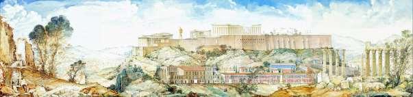
In the race for square meters, the image of the native place is replaced by a new, not too comfortable standard urban development, and it is the figurative component that has the most important influence on the education of love for the native city, streets, houses, makes a person take care of everything that is connected with the Motherland and many other socially important concepts. Fig. 2 (a, b) shows the reconstruction of ancient capitals. The greatness of the image of Athens is crowned by a sculptural image of the Virgin Athena, just as the Moscow Kremlin welcomes guests with golden domes.

Architecture has an impact on the formation of the personality of not one, but many generations, and the impact of the architectural image on a person cannot be overestimated, therefore its spiritual and cultural component is so important [2]. Figure 2 (c) shows the road

to the Ferapontov Monastery – one of the northern pearls of Russian Orthodoxy and an example of urban planning art. An important task in preserving the culture of our countryis the revival of the ancient heritage, the creation of archaeological parks, museums, and educational centers.

The figurative component in the construction of the city, the temple, housing and all urban structures had a significant impact on the formation of cities, ensembles, public and residential buildings. The unity of the systems of transport arteries, squares, public pedestrian spaces, arcades of palaces and parks, fences of squares and fountains was subordinated to the harmony of the relief, natural and climatic conditions and urban functions. All the elements equally participated in creating the harmony of intertwining structural elements, the purity of the quality of materials, the unity of geometric elements and the boundless imaginative understanding of the form [3].

The concept of an image in architecture fully absorbs its artistic and philosophical basis, collecting, as in a symphony orchestra, each instrument in a single harmonious sound. Figure 2 (a, b) presents reconstructions of panoramas of Athens and Moscow, Figure 2 (c, d) shows photographs of panoramas of Russian cities –the compositional unity of the temple ensemble is indisputable, this is how the recognizable «face» of the city is formed, which each of us carefully keeps in memory. This is due not only to the recognition of the place, so we «read» the history and realize the importance of the city.

Fig. 1 a) the Acropolis, a project of the student D. Shepetkov. project. MARCHI 1993,

b) Preparation of the concert stage in ancient Greek theater in Syracuse

c) temple complex at Agrigento (ancient Greek Akragas) d) Chersonese (City, Peninsula) was founded in 422-421 BC by colonists from Heraclea Pontica

c)

Fig. 2,

The urban planning art of ancient architects still serves as an example in the training of architects, but its figurative component, which has a clear structure and certain constructive characteristics, is increasingly being overlooked in textbooks. For example, the spatial structure of the ancient Greek acropolis, the sacred citadel, the agora or the forum, or other significant public spaces of the ancient city repeats the structure of cosmogonic myths inthe aspect in which mythological images are ordered in a logical sequence of events. Thus, the sacred (Panathenaic) road carries the ritual meaning of the movement connecting two worlds: the earthly («city of people») and the heavenly (acropolis), thanks to which a person gets the opportunity to participate in hierophany. The movement of the festive procession is

designed for the possibility of contemplating and «reading»the ensemble ofthe Acropolis, graduallydiscovering new images (Fig. 3a). Getting into the space of the holy city, the participants of the festive procession found themselves in front of the patroness of the city – Athena (Fig. 3b).

Russian cities have the same attractive force, indestructible and indelible by time. In the central part of Russia, in the ancient city of Yuriev-Polsky, for almost a millennium, visitors have been greeted by the calm grandeur of ancient temples (Fig. 3b). The balance of proportions, proportionality to a person, festive solemnity endow the ancient square of the city with properties inherent in eternal, indestructible monuments.

a) Reconstruction of the Athenian Acropolis by Leo von Klenze in 1846,

b) The heyday of the Kremlin. Vsekhsvyatsky Bridge and the Kremlin at the end of the 17th century, A.M. Vasnetsov.

Spatial landmarks of the Russian city. Ferapontov Monastery

d) Holy Trinity Sergius Lavra.

a) the Acropolis of Athens,

b) the Mikhailovo-Arkhangelsk Monastery in Yuriev-Polsky. Fig. 3

Russian Russian cities are united by the unity of the compositional solution (Fig. 2). The spatial landmarksofthe entrances totheancientGreekand Russian cities are similar in the scale of architectural elements, the location of the location, the significance of the location in space, the divine beauty and a sense of unity with the surrounding nature, the presence of the most important spiritual and protective dominants for the entire population at the same time. Thus, the golden armament of Athena-the virgin-defender (Fig. 3b), towering over the city, informed everyone approaching about the greatness, power and strength of the acropolis. Approaching Athens, every traveler saw from afar the golden helmet of the guardian and patroness of the city. The colorful picture evoked mythological images associated with the goddess, while the place of birth, residence and upbringing of the viewer did not matter, every resident of Ancient Greece knew all the myths from childhood.

Each fragment of the architectural space is an element of the figurative language of the ancient Greek architects, is the embodiment of an understanding of the

surrounding world, the boundless diversity and the surrounding reality at the same time. Religious buildingsthe most important spaces of the ancient Greek citywere the collective image and the fundamental center of the ideal representation of society about the cosmic harmony of the Olympic Pantheon. Ancient Greek architects managed to create an order system that served as the basis for the creation and development of European architecture for all subsequent millennia. This constructive system, endowed with a figurative component, served as the basis for the further development of Russian and European architecture.

The constituent elements of the image of an architectural ensemble are individual structures, details and structural elements, color ratios, angles of refraction of light, the quality of materials and many other factors. The impact of this image on a person is so strong that after two and a half thousand years, a large number of people travel great distances to touch the ruins of ancient temples. Two thousand years later, ancient Greek temple complexes serve as attractive sites for the creation of archaeological parks, museums, the development of tourism and cultural traditions (Fig.4 а,b).

a) the Parthenon,

b) the Delphic Tholos-the Temple of Athena Pronaia.

For us, ancient Greek culture is one of the most important sources of the richest European civilization –the basis of writing and grammar, including music, philosophy, art and architecture [6]. Until now, we use grammar, the foundation of which was laid in ancient Greece. Musical grammar, the name of notes, the creation of a sheet music mill and the basics of harmony of ancient Greek musicians are taught to children in schools with traditional classical music teaching [7]. Training in drawing and painting begins with the study of elements of the ancient Greek order and ancient sculptures. The ancient Greeks-the great rationalists and dreamers-used the system of calculating the area of a complex figure by dividing it into smaller ones long before Descartes formulated and published this system.

Ancient Greek architects had no equal in creating urban-planning ensembles, they paid great attention to the opportunity to admire the surrounding nature, creating view platforms on stairs, in palaces for the opportunity to admire the surrounding landscape. The ability to see and hear the beautiful is so necessary for every person, and this is why the characteristics of Greek and Russian temple complexes are so similar. The urban planning art and architecture of ancient Greek architects is associated with Russian architecture. Russian

cities were located on the banks of rivers and lakes –the main transport arteries available at any time of the year. The golden domes of Orthodox churches in Russian cities were landmarks, signs of power and spirituality, and the bells were a way of communicating about a holiday or an enemy attack (Fig. 2 c, d).

It is interesting that the diverse architectural space of the ancient Greeks for thousands of years has an indelible, vivid impression on the audience, which is enhanced in the ancient world by the movement of a ritual procession accompanied by music, dance movements, sports competitions. The events were illuminated by bright sunlight and the impact of the architectural image was enhanced by the play of light and shadow. The frieze of the temple repeated the dance movements of the procession (Fig. 5a), and the flutes of the colonnades emphasized the geometry of the image (Fig. 5b). The strength of the impact of architectural ensembles and individual elements on the viewer who took part in the festive procession was enhanced by the color and movement of the sun's rays. The diversity of ancient Greek architecture has collected and preserved for centuries an unlimited ideological meaning, which has absorbed into itslanguage a varietyofimages and the versatility of the surrounding world.

a) The Parthenon, the eastern side of the Ionian frieze of Cella «the offering of peplos to Athena». 442-438 BC,

Fig. 5

Ancient Greek temples, similar to each other in style, in general geometric and structural parameters, had a unique image, harmony of proportional proportions and the plot of bas-reliefs [5], while the image of each temple was individual and did not repeat itself. The genius of the great rationalists and dreamers-ancient Greek architects-is read in the simplicity of the form and complex geometry of each detail, in the play of light in the interior of the temple, the simplicity of the capital, the complex configuration of the details of the order and the direction of movement of the ritual procession.

The game of light-shadowrelations has been skillfully created in the architecture of ancient temples, a perfect example of the skillful use of light effects for training modern architects. When recreating ancient temples on the territory of Russia, it would be possible

to conduct an internship for architecture students without leaving the country. The creation of illusions of movement, obstacles and penetration in space was created by ancient Greek architects in each colonnade. In the minds of the audience, when looking at the Parthenon, the sense of an obstacle – an external wall-was lost, and at the same time it existed in the form of a «transparent», permeable barrier. This is the illusion of penetration, of knowledge of the «hidden», hidden world – the house of the deity. The structural supportthe bearing part of the order in the imagination of the master appeared as a kind of «as it were» open space. It should be borne in mind that the essence of the archaic worldview is that the architect does not mythologize, but on the contrary, deduces a certain image from the mythological world and materializes it in spatial forms

b) Erechtheion. The grace of the Ionian Order. 412-406 BC.

– architectural elements. Thus, the deceptively permeable outer wall of the Parthenon is an image of the Cosmos, which does not give away its knowledge, but allows you to «contemplate» its harmony (Fig. 4a).

Each element of the temple carries a whole world of mythological images, there is the mystery of the ancient East in the form of triglyphs, the grace of the movements of the goddess can be traced in the flutes of the Ionian order. This mystery is allegorically, strangely and meaningfully demonstrated on the facades of temples. The diversity of every detail of the Greek temple tells the audience about the whole world of human earthly life, his touch with the earthly world: metopes – in the form of a story about the exploits of Hercules (Fig. 6a) or tragic scenes of the struggle of

Lapiths with centaurs (Fig. 6b). The image of the hero, punished for resisting the Olympian gods, is found in the temple of Zeus in Akraganta. Here, in contrast to the traditions, the colonnade is replaced by a wall with half-columns, and the defeated Atlanteans hold the skypediment on their shoulders. Illuminated by the bright sun, the columns, merging with the surrounding space, dissolve into the blue of the sky and it seems as if their slender row is limitless. Here the open space of the colonnade is replaced by a blank wall, and the history of the city colorfully tells the events accompanying the construction of the complex and through the millennia the ancient defeated Atlanteans look at the visitors of the museum, silently telling about their exploits (Fig. 6b).

a) The metopes of the temple of Zeus in Olympia depict the exploits of Hercules. Athena helps Hercules to hold the sky instead of Atlanta

b) The Metope of the Parthenon temple. The battle of Lapiths with centaurs. Metope of the Parthenon

Fig. 6,

c) The defeated Atlantean supports the sky-frieze in the temple of Zeus in Akraganta.

architects in the XII century.(Fig. 7)

No less beautiful are the images of the facades of St. George's Cathedral in Yuriev-Polsky,

An excellent example of comparing the changing images of an ancient deity is the image of the ancient ancestral goddess on the pediment of the temple of Artemis in Corfu (Fig. 8 a) and a later example of female

beauty-the beautiful Venus of Milo (Fig.8 b). The image of the intercessor of the Russian land - The Vladimir Icon of the Mother of God is the oldest and most revered in Russia (Fig. 8 c).

created by

Fig. 7. Fragments of stone carvings of the St. George Monastery in Yurbev-Polsky. XII century.

a)

Fig. 8.

The preservation of history has a key role in the knowledge of the future, and understanding the image of the past millennia allows you to look into the very depths of the meaning of the past. Architecture is the most vivid material embodiment of the worldview of long-vanished generations that has been preserved for centuries. Reading the history of ancient Greek architecture and culture in general, we understand the depths of Europe's cultural traditions, its aspirations and dreams. The study of architectural images and possible reading options leads to an understanding of the architectural space, each element of the architectural language, the development and understanding of surrounding events.

Of course, the attempt to reconstruct the process of ancient Greek shaping is more than conditional, but such comparisons of architectural elements of the two cultures lead to the idea that the shaping and understanding of space are similar in many ways between the two peoples. This suggests the need for careful preservation and recreation of ancient monuments, the creation of museums for the preservation and teaching of classical art. The consistent creation of museums, the reconstruction of the most preserved interesting monuments of ancient Greek culture will affect the development of cultural and educational tourism, the construction of hotels, museums, the development of agricultural land and other related structures, the creation of handicrafts, art festivals, concerts.

OntheterritoryofRussia,almostallancientGreek policies were destroyed in different time periods. But the receiver of ancient culture was the centers of Orthodoxy-Chersonesos, where in the IX century the Grand Duke of Kiev Vladimir was baptized, the heyday of the principality of Feodoro in the southern part of the Crimean Peninsula. It should be remembered that many ancient cities destroyed by conquerors or natural disasters will not be revived, but they retain all the archaeological information about the layout in various periods of their development in its original form.

Thecultural,educationalandspiritualcomponents ofthearchitecturalimageofancientcitiesareimportant in the formation of the foundations and traditions of modernity. Tauric Chersonese, Bosporan Kingdom, Scythian Naples, Tanais, Panticopaeum, Kerkinida,

Shermonassa, Phanagoria preserve the ancient culture. Museums are being created on the territory of these cities, it is also necessary to create archaeological parks in all ancient settlements, create cultural and educational centers with libraries and museums. This will have a significant impact on the development of cultural and educational tourism, education and cultural development.

In the planning structure of the modern city, centuries, centuries, changes in culture and religion were intertwined in a single urban planning ensemble, but what is commonly called «The Spirit and image of the city» was not destroyed by time, but was only supplemented, transformed, giving birth to new images, linking them into a single multicolored carpet. What the city of the future will be like, what new incomprehensible images will arise in hundreds of years, we can only guess. I would like to preserve the grandeur of the ancient image that protects the spirit of the city, its traditions and foundations, which has its own complex structure and unusual fate.

REFERENCES:

1.Florensky P. A., investigations in the theory of art// Florensky P. A., priest. Articles and studies on the history of art and archaeology. – M.: Thought, 2000. –S. 79-421. (XLIII 1924. IV. 18, In the margins, pencil recording of the hand of P. A. Florensky: "the Ornament. Hypertrophy comp(azizia) and des(uccee). Machine". 152)

2.Kudryavtsev M. P.. Moscow – The Third Rome. Historicalandurbanresearch. M.,Trinity.,2007 -288с.

3.Mokeev G. I.. heavenly city of Holy Russia. M.; Itios. 2007 – 256с.

4.Shvidkovsky D. O.. Historical path of Russian architecture and its connection with the world architecture. Architecture, 2016 – 512с.

5.General history of architecture in 12 volumes, vol.1, M., 1970., S. 245

6.Dmitrieva N. A. Akimov L. I., Antique art, M. Children's literature in 1988. 256 p., Il

7.Мalaya E. V., Study of the units of architectural language (on the example of the ancient Greek orders). The dissertation on competition of a scientific degree Cand.architect 1997. 180 с.: ил. (Мalaya E. V.)

The pediment of the Temple of Artemis in Corfu, b) the Venus of Milo, c) the Vladimir icon of the Mother of God.

EARTH SCIENCES

INVESTIGATION OF ATMOSPHERIC DOMAINS WITH THE AID OF MATHEMATICAL MODEL OF THE GLOBAL BIOGEOCHEMICAL CARBON CYCLE IN THE BIOSPHERE

Tarko A.

Doctor of Physical and Mathematical Sciences, Professor of Mathematical Cybernetics Chief Researcher of the Dorodnicyn Computing Centre of the Federal Research Center «Computer Science and Control» of Russian Academy of Sciences

DOI: 10.24412/3453-9875-2021-70-1-10-22

Abstract

With the aid of mathematical model of global biogeochemical carbon cycle with a spatial structure and seasonal dynamics atmospheric C02 domains investigated. It is shown that domains which are the regions of low carbon dioxide concentration in the atmosphere arise as a result of the high photosynthetic activity of terrestrial vegetation in the interaction withthe circulatingatmosphere. Domains are graduallyoccupya several spatial zones of low CO2 concentration from one edge of the Earth's map to the other.

Keywords: Modeling of the biosphere, biogeochemical cycles of carbon, net primary production, atmospheric transport, CO2 concentration, CO2 domains, tube of trajectories, contour lines.

Nowadays numerous measurements the biosphere parameters are being carried out in the world, as well as mathematical modeling of the global carbon cycle. However, much in understanding the properties biosphere remains unclear by this time and one of that is the integral functioning of the carbon cycle. The use of new measurements results and modeling of the carbon cycle allows us to obtain and test hypotheses about the functioning of the biosphere within a single spatial model and consider the biosphere as if it were the biosphere itself. This allows us to develop and test hypotheses about the dynamic properties of the biosphere, as well as to put forward new ones and immediately test them. Only on global models can we perform computational experiments with the biosphere that allow us to

understand its holistic properties, provided that global experiments with the entire biosphere are impossible in reality.

Usually, when analyzing the seasonal dynamics of the atmosphere, the dynamics of CO2 concentration is analyzed by latitude, and then the results are compared at different latitudes (Fig. 1).The subsequent workconsists indeterminingthe distributionofCO2 maxima and minima at each latitude and determining how far the CO2 minimumis far fromthe photosynthesis maximum at the same latitude. This approach does not provide a holistic understanding of the spatial dynamics of CO2 in the atmosphere.

Fig. 1. The 3D picture shows results of measurement of CO2 dynamics in the atmosphere. We can see seasonal fluctuations of CO2 every year and the change in the amplitude of fluctuations during the year at any latitude and also for several years (1983-2007) at each longitude.

In this article, with the help of mathematical modeling of the biosphere the author presents the results of a spatial study of the dynamics of CO2 in the entire atmosphere. The results obtained by such modeling on a global spatial biogeochemical model of carbon dioxide with seasonal dynamics. The author perhaps was the first to identify and study six regions of low carbon dioxide content in the atmosphere and called then domains. This study is devoted to the investigation of the formation and movement of CO2 domains in the atmosphere as part of the biosphere processes.

The research tool is a spatial mathematical model of the global biogeochemical carbon cycle developed jointly with V. V. Usatyuk [6, 7]. Biotic and physicochemical processes of carbon transport in terrestrial ecosystems, in the ocean and in the atmosphere are modeled. The model has a spatial resolution with a size of4°x5°ongeographicalgrid,thetimeresolutionisone day. Each land cell is considered to belong to one of the 30 types of ecosystems in accordance with the classification [1]. The General Circulation Model (GCM) in the atmosphere and ocean is used as a source of climate data [12].

This model is a variant of a more complicated biogeochemical model of the global CO2 cycle, which has also a more detailed resolution of 0.5°x0.5° and is used to study the stability of the biosphere and to analyze global warming processes [3, 4, 5].

The equations describing the dynamics of carbon in the vegetation cover take into account the following phase variables: the amount of carbon in the biomass of leaves, the biomass of trunks and the biomass of roots. The amount ofcarbonin the assimilates and the amount of water in the upper meter layer of the soil are also taken into account. The specific intensity of photosynthesis is calculated using the Gaastra equation. Respirationofplantorgansandsoil alsoistakenintoaccount. Vegetation evapotranspiration is calculated using the Paynman-Monteith formula, which takes into account the energybalance ofthe moisture evaporationprocess.

In addition of GCM model special atmosphere block for calculating the transport of CO2 in the atmosphere has been developed. For this purpose, the convective-diffusion displacement of a small impurity of a passive gasinagivenspherical velocityfield was mathematically solved. The mathematical problem of convective-diffusion transfer of a small impurity of a passive gas in a given spherical velocity field is solved. Having its own transport unit allows the author to model the seasonal dynamics of CO2 concentration for

each climate scenario, without performing a laborious calculation of all climatic parameters using a complete climate model.

The "atmosphere-ocean" block [2] is designed to calculate the parameters of the carbon cycle in the ocean, as well as to determine the carbon fluxes at the interface between the atmosphere and the ocean.

The model is validated using measurements of climatic and biotic parameters, data on the concentration of CO2 in the atmosphere at monitoring stations [1, 8, 11]. A check of the coincidence with the data of the spatial model was also carried out [5].

Computational experiments with satisfactory accuracy confirmed the course of the production process in land vegetation, in the decomposition of soil organic matter in most cells and allowed to obtain calculations of changes in the concentration and transport of CO2 during the year for all selected cells, as well as for latitudinal zones. Calculations have shown that the theoretical curves and measurement data are close both in amplitude and phase, i.e. this model satisfactorily reproduces the overall dynamics of CO2 in the atmosphere.

The computer simulation confirmed the hypothesis that the main causes of seasonal CO2 fluctuations are the photosynthetic activity of highly productive terrestrial vegetation, which releases a large amount of CO2 from the atmosphere, and also “pulls” CO2 from regions with lower photosynthesis values thousands of kilometers away.

In the model, the transfer of air masses along the latitude is much faster than in the meridional direction. Accordingly, the alignment of the CO2 concentration along the latitude also occurs much faster. For this reason, it is generally accepted in many studies that the composition of the atmosphere changes only in the meridional direction, but is the same throughout the latitude.

With the help of modeling, the author found stable structures in the atmosphere consisting of CO2 with a reduced CO2 content, which regularly occur in the atmosphere throughout the year. These structures are called domains. Theyoccur in the atmosphere in different places at different times of the year, they contain local CO2 minima, and as they develop, they move and increase in size [6, 7]. 6 domains have been identified that occur in the following regions: 1) Europe and Siberia, 2) North America, 3) Amazonia, 4) Central Africa, 5) Indochina and 6) Australia and Indonesia (Fig. 2).

Fig. 2 Location of domains on a map of the Earth. 1 - Europe and Siberia, 2 - North America, 3 - Amazonia, 4- Central Africa, 5 - Indochina, 6 - Australia and Indonesia.

Domains appear as regions of an abnormal decrease of CO2 concentration against the background of its general dynamics, which have existed ordinary for a several months.

The phenomenon of domains was investigated using simulating experiments on the model which is described here. It was found that the main cause of the emergence of domains are production processes in highly productive ecosystems of terrestrial biota.

The atmospheric circulation has a significant effect on the characteristics of domains and their dynamics, due to which the domains are usually shifted towardstheleewardborderoftheregions.Thus,theyturn out to be “tied” to regions occupied by highly productive ecosystems, but do not occupy a strictly defined position above the surface of the Earth. Their position and shape is determined bythe movement of air masses in the considered land region and depends on the inten-

sity of carbon absorption by vegetation. Due to variations in climatic parameters, each year the vegetation season passes with different characteristics, therefore the shape of domains varies slightly in different years. As already mentioned, usually when analyzing seasonal dynamics, the atmospheric CO2 concentration is averaged over latitude, and these curves are compared at different latitudes. In this paper, the author conducts a more complex analysis – there is a study the spatial movements of domains at the background of seasonal fluctuations in atmospheric CO2. One of the areas of research was the analysis of the spatial dynamics of processes in latitudes. To do this, there were constructed graphs representing the tubes of trajectories of atmospheric CO2 located at the same latitude during the year in each of 12 months for all longitudes (5 degrees ofgeographicalcoordinates).Thus,tubesoftrajectories were constructed for latitudes N 60°, N 50°, N 30°, N 18°, S 10°, S 30° (Fig. 3).

Fig. 3. Tubes of the trajectories of atmospheric CO2 concentration during the year at latitudes N 60°, N 50°, N 30°, N 18°, S 10°, S 30°. Each tube of the trajectories gives 72 curves of CO2 concentration of all longitudes (along 5 degrees) at given latitude. The vertical axis show atmospheric CO2 concentration in particles per million (ppm). The horizontal axis shows month numbers.

For all latitudes of the Northern Hemisphere from N 60°toS 10°, minimumofconcentrationareobserved in September-October (for latitude S 10°, individual minima of the tube of trajectories reach November). Only at latitude S 30° do the values of the curves come in December-January to a state close to stationary.

The originofthese minima is explained bythe fact that highly productive forest ecosystems of the Northern Hemisphere, located in the latitudinal range from N 40° to N 60°, absorb CO2 from the atmosphere in summer. The discrepancy between the time of the minimum of CO2 and the maximum of productivity by a month and a half is determined by the nature of the dynamic process in which the absorption of CO2 from the atmosphere has a maximum, but it shifts from the movement of air masses.

It should be noted that the far the south of the zones of the production process, the later the minimum is reached in the months indicated. The explanation of the results is that the zones ofthe active productionprocess “attract” CO2 from neighboring atmospheric regions, and the effect of attraction extends to the north and south, spreading to the southern hemisphere.

It should be noted that ecosystems lying in the zone of boreal and subboreal forests of the Northern Hemisphere are of decisive importance for the occurrence of CO2 minimum. Ecosystems of the tropical zone,havinghigherproductivity,exhibit weakseasonal variability, which does not allow influencing the formation of the time of onset of minima.

These highly productive zones are also present in the Southern Hemisphere, but they have much smaller sizes and power. The tubes of the trajectories S 10°, S 30° show unique complicated behavior At latitudes S 10° – 30°thereisadoubleprocess.Oneprocessisthe aforementioned “pulling” of CO2 by ecosystems of the Northern Hemisphere with a minimum of CO2 in September – October, and the other is the absorption of

CO2 by “their” ecosystems with a minimum in March – April. This can be seen from the CO2 minimums on the tubes of trajectories S 10°, S 30°, reached in March – April, which also obviously lag is two months behind the maximum productivity in this hemisphere.

The reason for the large difference in the spread of CO2 values at the times ofthe minimuminthe indicated months is unclear – at the latitude S 10° the “thickness” of the trajectory tube is much larger than at S 30° vary greatly at different longitudes. This case requires further, more careful research in modeling.

How are these results related to the previously identified six spatial domains? We can say that the domains are located inside the tubes of the trajectories of concentrationofthecourseofatmospheric CO2 concentration during the year at latitudes. Indeed, each tube of trajectories means, as it were, an instant cut of 72 longitudes in each of the 12 months of the year. This procedure is not able to take into account domains that are spatial formations inthe atmosphere. The consideration of the trajectories brings us closer to the assumption of instantaneous latitudinal mixing, accepted by the world when analyzing atmospheric CO2 monitoring data, but still does not reach this point.

Next, “surfaces” that form CO2 concentration values were examined. A series of computational experiments were performed with the condition that vegetation is occupying only one of several continents. For this purpose, the division of the land surface into four regions by geographical type is used: 1) Eurasia, 2) North America, 3) South America, 4) Africa. The outlines and boundaries of all areas are shown in Fig. 4. For each region the modeling was carried out until a periodic stationary regime was established, provided that the amount of carbon in all the system was constant. For each day, maps with isolines of atmospheric CO2 concentrationand formed CO2 surfaces were constructed using the Surfer program.

Fig. 4. Map of selected areas for partitioning the territory for modeling

We begin the studyby analyzing processes in Eurasia. Vegetation season here begins in April – May. Usually, the first few days are accompanied by a uplift of CO2 into the atmosphere. This is due to the fact that the respiration of the soil, trunks and tree branches exceeds photosynthesis that occurs in the newly emerged leaves. Several days after and for the entire growing season, the CO2 uplift becomes directed from the atmosphere to the biota of the selected area. The following are maps with isolines and surface concentrations

of atmospheric CO2 calculated using the model, calculated on the 180th, 200th and 260th days.

In fig. 5 (day 180), we see a noticeable decrease in CO2 lying in the range 0° – 180° E and a slight decrease in the northern part of the Western Hemisphere are also visible. This is due to the emergence of a domain (local minimum) upon absorption of CO2 by biota. The domain immediately begins to expand due to an increase in the intensity of the production process and turbulent diffusion of carbon dioxide in the atmosphere and is

carried away by the winds mainly to the east and partiallytothesouth.Withthedevelopmentofthegrowing season, the domain continues to grow in size, while the resulting "funnel" from CO2 becomes deeper, its width increases in the latitudinal and longitude directions. The latitudinal direction is much larger, because the

zone occupied by photosynthesis, increasing in all directions, especially grows towards the east. The main transfer of CO2 to the east comes from the fact that in the atmosphere due to the rotation of the Earth there is a shift of air masses to the east.

Fig. 5. Eurasia, day 180. Map and surface of CO2 concentration. A dip lying at 0-180° E and a slight decline in the northern part of the Western Hemisphere are visible. CO2 concentration decreases markedly from the North Pole to the South Pole.

The zone of lowered CO2 gradually reaches the Western Hemisphere, and on the map by the 200th day (fig. 6) a decrease in CO2 occurs in its left part. Two minimums are visually obtained – one reaches the border of the Eastern hemisphere (on the right of the map), the other moves from the left border of the Western hemisphere and goes to east (to the right). Then, as the size grows and shift eastward to 260 days, thentwo sections gradually merge into one wide zone (Fig. 7),

reaching the North Pole in latitude to the north, and 2530° N in the south. Gradually, a large wide and deep band of reduced CO2 is obtained, while the decrease in the surface of CO2 reaches 25° S and there is also an increase in CO2 concentration in the circumpolar part of the Southern Hemisphere, due to the fact that the amount of CO2 in the simulated system does not change, and excess CO2 is transferred to the South.

Fig. 6. Eurasia, day 200. Map and surface of CO2 concentration. A dip lying at 0° – 180° East. and a noticeable decrease in CO2 in the northern part of the Western Hemisphere are visible. CO2 concentrations in the northern and southern parts of the Earth are approximately equal.

Fig. 7. Eurasia, day 260. Map and surface of CO2 concentration. Two CO2 minima are visible at the edges of the Eastern and Western hemispheres. Both minima are in a wide zone of low CO2 concentration formed by vegetation of biota. The CO2 concentration is rapidly growing from a wide zone of lower values at the North Pole to the South Pole.

The indicated circumstances are visible in fig. 8, which shows the difference in concentrations between 140 and 240 days of the year. On the map of contours and the surface of CO2 formed by the difference in CO2 concentrations, a minimum is seen that lies in the eastern part of the Northern Hemisphere, with a decrease in the CO2 difference of -10 ppm. In the western part of the map and the surface, a section of lowering CO2 is

visible coming from the Eastern Hemisphere. The difference in CO2 concentrations fromthe northern part of the Earth increases markedly to the southern part. The zone of negative difference lies from the North Pole to 25° S. Note that in the system under study, the difference inCO2 concentrations does not reach negative values due to the fact that, as was mentioned, the amount of CO2 in the biosphere is constant and all variables cannot become negative.

Fig. 8. Eurasia. Map and surface of CO2 concentration formed by the difference in CO2 concentrations in days 140 and 240 are presented. One can see a minimum of CO2 lying in the eastern part of the Northern Hemisphere, with a (-10) ppm of CO2 concentration. In the western part of the map and the surface, a section lowering of CO2 is visible coming from the Eastern Hemisphere. The difference in CO2 concentrations from the northern part of the Earth increases noticeably to the southern part. The zone of negative difference occupies the space from the North Pole to 25°S

Fig. 9-10 shows maps of the "North America" scenario withisolines and surface ofatmospheric CO2 concentrations on the 200th, 240th, and 260th days. In general, we obtained qualitatively similar results with the "Eurasia" scenario. The difference is that the source of the production process is located to the west, while the territories occupied byvegetation is less space in longitude, and in latitude is closer to the south. Fig. 9 shows

a similar to fig. 5 noticeable decrease in the concentration of CO2 in the area by the 200th day of the year. Then, over time, the zone of reduced CO2 gradually reaches the edge of the Eastern Hemisphere and the border of the Western hemisphere. At the same time, two minima do not appear on the map, there is no place for this on the territory of America.

Fig. 9. The scenario “North America” Day 200. Map and surface of CO2

The influence of the domain is such that the concentration of CO2 is reduced towards the North Pole. The area with a minimum of CO2 gradually turns into one wide zone (Fig. 10-11), reaching the latitude to the north – the North Pole. Gradually, a large wide and

deep band of reduced CO2 is obtained. In this case, just as in "Eurasia", the absorption of CO2 in the domain leads to the fact that the direction of the north – south shift of the CO2 concentration significantly decreases towards the North Pole.

Fig. 10. The scenario "North America" Day 240. Map and surface of CO2

Fig. 11. Scenario "North America" Day 260. Map and surface of CO2

In Fig. 12-13, the results of the “South America” scenario calculations with contours and surface of atmospheric CO2 concentration on the 160th and 50th days are given. Fig. 12 shows noticeable decrease in CO2 concentrationinthezone ofequatorialtropicalforests, from which territories of low CO2 concentration

go west and east to borders of the map. Another case is shown in Fig.13: the zone of reduced CO2, still occupying tropical forests, gradually decreases towards the producing vegetation of the Southern Hemisphere, while there is also a sharp decline of CO2 in zone W 50° longitude to the South Pole.

Fig.12. Scenario "South America". Day 160. Map and surface of CO2

Fig.13. Scenario "South America". Day 50. Map and surface of CO2

Fig. 14 shows the calculation map of the "Africa" scenario with isolines and surface of atmospheric CO2 concentration on day 320. Fig. 14 shows the influence of the equatorial tropical vegetation of Africa. A strong decrease in the CO2 concentration in the tropical vegetation zone is visible, and a wide band of reduced CO2 concentration is visible, extending to the North Pole and reaching the eastern and western borders of the

map. Inthis scenario, the same effects that have already beenplayed arereproduced.Thevegetationsouthofthe tropical zone is particularly affected. At the same time, the minimum of CO2 in the Northern part of Africa is accompanied by a gradually decreasing concentration of CO2 in the Southern Hemisphere. There is a stronger change inthe directionofthe CO2 concentrationof vector "Northern – Southern" hemisphere.

Fig.15. Scenario "Africa". Day 50. Map and surface of CO2

Fig. 16 shows isolines of the CO2 of the "Africa" scenario at map of difference between 320 and 140 days. It can be seen that almost the entire land area between the poles has a reduced concentration. An exception is an uneven strip with a protrusion near the equator and a small area at the South Pole. Note that this

figure demonstrates not only a change in the direction of the vector of the shift of the CO2 concentration "north – south", but manifests moments when its direction goes from the equatorial part to both poles of the planet.

Thus, for the first time it was shown that each of the considered continents leads to the formation of significant territories involved in the process of CO2 transport in the atmosphere, exceeding half the planet’s surface. Domains formed over the continents gradually occupy a wide latitudinal band of low CO2 concentration from one edge of the Earth's map to the other. This strip can occupyalmost the entire hemisphere from one continent and enter to another. At this case, during the year, the direction of CO2 reduction can be changed - it can be mainly directed to the Northern Hemisphere fromthe SouthernHemisphere, and visa versa. It is also possible that the decrease in concentration occurs from the equatorial region with a simultaneous decrease to the North Pole and to the South Pole.

From the simulation experiments, it became clear that the power of the processes of air mass movement associated with the photosynthetic activityof terrestrial vegetation is higher than when forming the interaction of two neighboring continents, based on the values recorded at monitoring stations. The curves of the dynamics of CO2 in the atmosphere are formed not only by two neighboring continents, but by almost all the continents of the Earth. The results of the calculations showed that the formationofthe values ofthe CO2 minima strongly depends not only on the vegetation of the nearest continents, but on several at once.

Theusualpractice, whenfirstlytheclimateandthe distribution of CO2 in the atmosphere are calculated, and then the calculations of the vegetation production process are performing with a constant or slightly

changing atmospheric CO2 concentration, may be insufficient in some real situations. In particular, with severe violations of the production process in local or large regions on the land are. Examples can be cases of strong warming of the atmosphere during global warmingorcalculationsoftheconsequences undersomescenarios of a limited Nuclear Winter.

It is known that during the vegetation process, air masses bypass the Earth several times along the latitude. This means that the simulated CO2 flow curves are the result of a complex geophysical process of CO2 dynamics inatmosphere.However, what is therelationship between the properties of the domain dynamics identified here and the fact of multiple "round-theworld travel" of air masses during the year remains to be determined.

The author has a pleasure to expresses gratitude to Vladimir Usatyuk who helped author to carrying out computer calculations for this article.

REFERENCES:

1.Bazilevich N.I., Rodin L.E. Maps of productivityof the biological cycle ofthe maintypes ofland vegetation // Proceedings of the All-Union Geographical Society.- 1967.- T. 99.- N 3.- p. 190-194. (In Russian).

2.Pervanyuk V.S. Tarko A.M. Modeling the Global Carbon Cycle in an Atmosphere-Ocean System. // Mathematical Modeling, 2001, v. 13, No. 11, p. 1322. (In Russian).

3.Tarko A.M. The global role of the atmosphereplants-soil system in compensating for impacts on the

Fig. 16. The scenario "Africa". Isolines of the difference of the CO2 concentrations between 320 and 140 days

Norwegian Journal of development of the International Science No 70/2021

biosphere. //Reports of the Academy of Sciences of the USSR. - 1977. - Vol. 237. - No. 1. - pp. 234-237.

4.Tarko A.M. Investigation of global biosphere processes withthe aid ofa global spatial carbondioxide cycle model. -SixthInternational CarbonDioxide Conference, Tokohu University, Sendai, Japan, 2001, V. 2. p. 899-902.

5.Tarko A.M. Anthropogenic Changes in Global Biosphere Processes. Mathematical Modeling. - M: Fizmatlit. 2005. - 232 p. (In Russian).

6.Tarko A.M., Usatyuk V.V. Modeling of the globalbiogeochemicalcarboncycletakingintoaccount seasonal dynamics and analysis ofthe dynamics of CO2 concentration in the atmosphere. // Reports of the Russian Academy of Sciences. 2013, V. 448, No. 6, p. 1-4. (In Russian).

7.Tarko A.M., Usatyuk V.V. Investigation of regional spatial structures in a model of the global biogeochemical carboncycle withseasonal dynamics. // Bulletin of environmental education in Russia. 2016, No. 1, p. 6-9. (In Russian).

8.Tselnicker Yu.L., Malkina I.S., Kovalev S.N., Chmora S.N., Mamaev V.V., Molchanov A.G. The growth and gas exchange of CO2 in forest trees. Moscow: Science. - 1993, 253 p. (In Russian).

9.Chan Y.H., Olson J.S., Emanuel W.R. Simulation of land-use patterns affecting the global carbon cycle. // Environmental Sciences Division. Publication N 1273, Oak Ridge National Laboratory, 1979.

10. Earth System Research Laboratory (ESRL), Map of Observation Siteshttps://www.esrl.noaa.gov/gmd/dv/site/site.php?code= WBI - (accessed: 06/22/2019)

11. Leemans R., Cramer, W.P., 1990. The IIASA database for mean monthly values of temperature, precipitation and cloudiness of a global terrestrial grid, // WP-90-41. IIASA, Laxenburg, Austria, 348 pp.

12. Schlesinger M.E. Simulating CO2-induced climatic change with mathematical climate models: Capabilities, limitations and prospects. Proceedings: Carbon Dioxide Research Conference: Carbon Dioxide, Science and Consensus. Coolfont Conference Center, Berkeley Springs, 1983. ASSESSMENT

Abstract

С.А., Кахраманов С.Г., Кулузаде А.Е. DOI: 10.24412/3453-9875-2021-70-1-22-25

Nakhchivan Autonomous Republic for the preservation of the ecological situation, its possible stabilization, long-term reclamation plans, based on the materials of the soil zones, the method of assessing the soil cover and assessing the landscape complex

The problem of rational use and protection of each hectare of land requires knowledge of all the features of smallandlarge unitsoflandscapecomplexes.Great importanceis alsoattached tothecomplexsoil,inother words, ecological characteristics of the territory. This line of research is of great theoretical importance.

Inour studies, special attention was paid to the compilationof correlations betweenthe productivityofnatural plants and the assessment of soil complexes.

Аннотация

Нахчыванская Автономная Республики

территории. Такого направления исследования имеет очень большое теоретическое значение. В проведенных нами исследованиях особое внимание уделялось составления коррелятивных отношений между урожайности естественных растений и оценки почвенных комплексов.

Keywords: appraisal, land cadaster, irrigated, agromelioration, heavy loamy Ключевые слова: бонитировка, земельный кадастр, орошаемый, агромелиорация, тяжелосуглинистый

Материал и методика Исследовательская работа проведена на 550275 га земельной площади Автономной Республики. Оценки почвенных комплексов это сравнительная качественная характеристика почв, коррелирующая с продуктивностью естественных растений. Исследованиями по оценки почвенных комплексов занимались Волобуев в соавторстве. (1967, 1973), Мамедов (1968), Крупеников в соавтор. (1971), Мамедов (1979, 2002, 2005), Мамедов, Гаджиев (2010), Мамедова (2002), Гаджиев (2010, 2015, 2020)

При оценке почвенных комплексов сельскохозяйственных, лесных и кормовых угодий нами использованы (Методические указания по бонитировке почв кормовых угодий Азербайджанской ССР, 1978, Методические указания по бонитировке почв в целях земельного кадастра Азербайджанской ССР, 1979, Методическое руководства по оценке плодородия почв лесных угодий Азербайджанской ССР, 1980) [4]. Объектом исследований служили Сероземные, Сероземы аллювиальные, Лугово-сероземные орошаемые, Сероземно–луговые орошаемые почвы, Коричневые (каштановые) почвы и под культурными растениями. Начиная с апреля месяца и до конца октября собрано около 150 почвенных образцов. Почвенные образцы было взято отдельно от из слоев 5-10 см и 10-20 см глубины почв. Войлокообразных водорослевый комочки отдельно собрано от поверхности почв и под высшие растения [6, 9, 11, 15]. Атакжеэто позволяетболее точноопределить пригодные места выращивания то или другой сельскохозяйственной культуры и провести агромелиоративные мероприятия, направленные на улучшение низкокачественных почв. Результаты исследований Сероземные почвы. В равнинной части автономной республики сероземные почвы занимают обширные пространства. Где распространены эти почвы, там и характерен наиболее сухой, жаркий и континентальной климат [1, 3, 5, 10].

Содержание гумуса незначительно. Сероземное почвы образуясь полынно-эферемовой полупустынной растительностью на более однородных суглинистых отложениях, протягиваются и в центральную часть равнины. Все указанные признаки относятся к обыкновенным сероземам почвам. Структура почвы комковатая, крупнокомковатая. Гранулометрический состав глыбистый, на глубине 70-100 см почва становится бесструктурной. Корни естественной растительности доходит до глубины 100-125 см. Эти почвы бедны гумусом, его количество доходит до 1,9%. Вниз по профилю количества гумуса уменьшается. Валовой азот очень малого-до 0,1%. Соотношение C/N-6,9-8,3. Гранулометрический состав этих почв легко и среднесуглинистый. Физической глина составляет 20-45%, а илистая фракция-9,26. Сумма поглощенных оснований составляет 14-23 мг.экв на 100 г почвы.

Сероземы аллювиальные. Эти почвы распространены в Шарурской равнине, вдоль р. Арпачай и больших каналов, развиты в с. Неграм Бабекскогорайона.Основнымипризнакамиэтихпочв являются пестрота гранулометрического состава отдельных слоев и серая окраска в верхнем профиле. Ниже 50-60 см окраска становится серо-бурой. Содержание гумуса в этих почвах 0,3-1,1%; валовой азот до 0,06%. Физическая глина составляет 21,4-29,9, а илистая фракция 6-12%. Лугово-сероземные орошаемые почвы. Эти почвы распространены в условиях высокого увлажнения. Окраска верхнего горизонта буровато-серая, а ниже темнее, структура почвы до 60 см комковатая. Сложение плотноватое и плотное. Эти почвы богаты полуторными окислами. AL2O3 составляют 16,0-18,9%. Гранулометрической составу средне и тяжелосуглинистые. Сумма физический глины 25-31 %, и илистая фракция 89%. Лугово-сероземные орошаемые почвы не засолены. Они насыщены поглощенными основаниями, сумма которых равна 25,4 мг.экв [1, 3, 5, 10]. Сероземно–луговые орошаемые почвы. По морфологическим признакам эти почвы близки к типичным луговым. В растительный покров здесь важную роль играет луговая травянистая группировка. В этих почвах содержание гумуса 1,7-2%, местами до 2,5%. По глыбистый, а ниже структура слабеет. По гранулометрическому составу они тяжелосуглинистые и глинистые. Физический глины содержится 60-70%. Эти почвы не засолены. Они наиболее насыщены поглощенными основаниями. Величина емкости поглощения 30-33 мг.экв. Коричневые (каштановые) почвы. В Азербайджанекоричневые(каштановые)почвыразвиты в области сухих степей и занимают широкую полосу предгорья и низких гор. Зона этих почв на восточных и северо-восточных склонах Малого Кавказа по М.Э. Салаеву (1953), охватывает полосу низких гор и предгорий с умеренно теплым полусухим и полувлажным климатом, где преобладает степная растительность. На территории автономной республике горнокоричневые (каштановые) почвы распространены в предгорно-шлейфовой полосе и занимают главным образом межгорные пониженные элементы рельефа, часто неширокими полосами они протягиваются по направлению к равнине. В связи с благоприятными условиями рельефа эти почвы с давних времен используются под орошаемые земледелие. В условиях автономной республики часто наблюдаются нижеследующие подтипы коричневых (каштановых) почв. В естественных условиях они формируются под сухой степной растительностью. Из почв равнинной части Нахчыванской АР коричневые находятся в лучших условиях для накопления гумусовых веществ. Верхний горизонт их характеризуется коричневой окраской с сероватым оттенком. Ясно выраженная коричневая окраска наблюдается в подпахотном горизонте, ниже 55-65 см она приходят в бурую, а затем (ниже 90 см) становится желтовато-

палевой. Структура почв комковатая, ниже 50-60 см комковатость теряется. В равнинной части автономной республики распространены лугово-коричневые почвы. Эти почвы используются под посевы сельскохозяйственныхкультур. В ихпрофиле наблюдаются ржавые и сизоватые пятна. Гранулометрический состава тяжелосуглинистый, часто глинистый. В восточной части территории этой же полосы встречаются лугово-коричневые почвы. Здесь наблюдается луговой тип почвообразования, важную роль в не играют грунтовые воды пойменной полосы, а также разливы рек. Коричневые почвы равнинной части богаты полуторными окислами. На пахотном горизонте AL2O3 составляет 16,8 %, а ниже увеличивается 1% больше. Содержание Si02 и Fe203 остается низменным. В давноорошаемых коричневые почвах гумуса содержится в среднем 3,2 %, валовой азот 0,16-0,17. Отношение C/N по всему профилю равно 8,7-13,8. Гранулометрический состав этих почв средне и тяжелосуглинистый. Сумма поглощенных оснований 19-29 мг. экв. pH-7,6-8,3. N/NO3 5,7 мг/кг и N/NH3 –до 23,3 мг/кг, подвижный P2O5 20-60 мг/кг, обменный калий-250-230 мг/кг. Светло коричневые (каштановые) почвы. Распространены в предгорно-шлейфовой полосе ниже коричневых. Эти почвы встречается также в повышенных элементах мезорельефа и формируются под полынно-злаково-эфемерной растительностью. Светло-коричневые (каштановые) почвы отличаются от типичных коричневых почв равнины осветленным профилем, более близким залеганием к поверхности карбонатных новообразований, бедностью гумуса и др. признаками. Окраска в ниже 40-50 см палевая или буро палевая. Структура комковатая ниже 50-60 см это исчезает. Гумус в этихпочвахсоставляет0,5-2,9%,валовойазоттоже немного. Эти почвы высококарбонатные. Нитратный азот содержится 3-6 мг/кг; аммиачный азот 1620 мг/кг; pH 7,4-8,3; подвижной P2O5 24-25 мг/кг; обменный калий 260-380 мг/кг и т. д. Валовой состав этих почв по профилю не изменяется средне и тяжелосуглинистые по гранулометрическому составу. Светло коричневые (каштановые) давноорашаемые почвы. Эти почвы являются одним из плодородных и издавна используются в сельском хозяйстве. В результате интенсивного орошения и обработки почв сильно изменились. Окраска этих почв ниже переходит в буровато-коричневую, а на глубине 60-80 см постепенно в палево-бурую. На территории Бабекского района в южной части эти почвы встречаются в виде солонцеватых разностей. Отличительные признаки этих почв светлая окраска, трещинноватость гор. В этих почвах содержание полуторных окислов высокое по профилю и почти не меняется. Гумус 1,3-2,0 %. Эти почвы высококарбонатные, среднесуглинистые, но встречаются тяжелосуглинистые и глинистые разности. Количество физической глины в верхнем горизонте в пределах 40-50%. Илистые частицы до 26

70/2021

%. Сумма солей в этих почвах менее 0,16%, значит эти почвы не засолены. Сумма поглощенных оснований составляет 19-23 мг.экв на 100 г почвы. Светло коричневые (каштановые) орошаемые почвы. В Нахчыванской АР вделаны также светло-коричневые (каштановые) орошаемые почвы. Эти почвы недавно используются в сельском хозяйстве и еще не очень изменены под влиянием обработки и полива. Структура этих почвах комковатая. Характерно близкое залегание карбонатов. Гумус немногий более 2%, высококарбонатный. Физический глины содержится 45-60%, илистой фракции 12,26%. Поглощенные основания составляют 20-22 мг.экв.

Внизу составлено список, жизненные формы, экологии и активности водоросли, распространенный в почве. 1. Водоросли, найденные в поверхности почв: а) в коричневым почве, б) в сероземной почве. 2. Внутри почв: а) коричневым почве, б) сероземным почве. 3. Выделители слизи. 4. Азотофиксаторы. 5. Облигатные автотрофы, Nпойкилоксерофиты. 6. Ксерофиты. 7. Засухоустойчивый. 8. Светолюбивый, засухостойкий. 9. Доминанты. 10. Субдоминанты [2, 8, 12, 13, 14].

Отдел Cyanoprokaryota: Род: Cylindrospermum F.T. Kützing, 1843 Et al Bornet and FlahaultCylindrospermum muscicola (Bory) F.T. Kützing, (1; 3), Cy. licheniforme (Bory) F.T. Kützing (1, 3), Cy. stagnale (F.T. Kützing) Bornet et Flahault (1, 3), Род: Anabaena Bory et al Bornet et al Flahault de Saint-A. cylindrica E. Lemmermann, 1896 (1, 3, 5, 8), A. variabilis F.T. Kützing (1, 4, 5, 8), Род: Synechococcus Naegeli, 1849-Synechococcus aeruginosus Naegeli, 1849 (1, 2), Sy. cedrorum C. Sauvageau, 1892 (2, 7), Род: Microcystis F.T. Kützing-Microcystis pulverea (Wood) Forti emend Elenkin f. pulverea (1, 2, 3, 8), M. parietina (Naegeli) Elenkin (1, 3, 7), Род: Microcoleus F.T. Kützing -Microcoleus vaginatus F.T. Kützing (1, 3), Род: Scytonema C.A. Agardh- Scytonema hofmanii C.A. Agardh (1, 2, 3), Род: Phormidium F.T. KützingPhormidium uncinatum C.A. Agardh Gomont (2a), Ph. autuminale (C.A. Agardh) Gomont (2, 7, 9), Ph. tenue Menegh. Gomont (2a, 5, 10), Ph. mole F.T. Kützing Gomont (2), Род: Gloeocapsa (F.T. Kützing)Gloeocapsa varia F.T. Kützing Gomont (2), Род: Oscillatoriaceae (Kirchner) Elenkin-Oscillatoria deflexoides Elenkin, Kossinskaja (1b, 3, 6), O. subtilissima F.T. Kützing (1, 2, 6), Oscillatoria chlorina F.T. Kützing Gomont (2, 9), Род: Lyngbya C. AgardhEtal Gomont-Lyngbya martensiana Meneghini (2), L. nigra C.A. Agardh (1a,3), L. spiralis Geitler (1a, 2a, 3), L. limnetica F.T. Kützing (2), Род: Microchaete Thuret et al Bornet-Mycrochaeta tenera f. minor Hollerb. (1, 2, 3), Род: Calothrix C. Agardh et al Bornet-Calothrix elenkinii Kossinskaja (1a, 2, 4), Ca. gracilis F. E. (1, 2, 3, 4), Nostoc Elenkin: Nostoc microscopicum (Carm.) Elenkin, Род: Schizothrix F.T. Kützing-Schizothrix arenaria (Berk. Gomont) (1,2, 3), Sch. muelleri Naegeli (1a, 2a), Род: Tolypothrix F.T. Kützing et al Bornet-Tolypothrix tenuis F.T. Kützing f. tenuis (1a, 3, 7),

Отдел Chlorophyta: Род: Ankistrodesmus CordaAnkistrodesmus braunii (Naegeli) Collins (2, 5, 8), Actinochloris sphaerica Korsch. (1, 5, 10), Род: Chlorella Beyerinck-Chlorella vulgaris Beijer. (1, 5, 9), Род: Chlamydomonas C.G. EhrenbergChlamydomonas konferta Korsch. 1, 5, 8), Ch. minima Korsch. (1a, 5, 8, 10), Ch. korschicoffi Pasch. (1a, 5, 9), Ch. polychloris Korsch. (1a, b, 5, 8, 9), Ch. sectilis Printz. (1, 5, 8, 9), Род: Closterium NitzschiaClosterium kuetzingii Breb. (1, 5, 10), C. ulna Focke (1a, b), Род: Chlorhormidium Fott-Chlorhormidium flaccidum (F.T. Kützing) Fort var. flaccidum (5, 10), Род: Cosmarium Corda et al Ralfs-Cosmarium regulare Schmidle (5), Род: Chlorococcum FriesChlorococcum humicola (Naegeli) Rabenh. (1a,5), Род: Scenedesmus F.J.F. Meyen-Scenedesmus guadricauda (Turp.) F.T. Kützing (5, 8, 10), Род: Cylindrocystis Meneghini et De Bary-Cylindrocystis brebissonii Menegh. f. brebissonii (2, 3, 5), Род: Chlorosarcina Gern.-Chlorosarcina minor (Gern.) Horndon (2, 5), Род: Ulothrix F.T. Kützing-Ulotrix variabilis F.T. Kützing (1a,b, 5, 8).

Tədqiqatlar nəticəsində torpaqların alqosinuziyasının əsas komponentlərinin 36 takson göy-yaşıl yosunlardan, 17 növ isə yaşıl yosunlardan təşkil olunduğu aşkar edildi. Növ sayına görə Nostoc, Lyngbya, Anabaena, Phormidium, Chlamydomonas cinsləri üstünlük təşkil edirlər. СПИСОК ЛИТЕРАТУРЫ:

1. Алиев Г.А., Зейналов А.К. Почвы Нахчыванской АССР. Баку: Азернешр, 1998, 235 с

2. Бачура Ю.М. Цианобактерии почв Гомельского региона // Материалы докладов II Международной научной школы-конференции, 16–21 сентября 2019 г., Сыктывкар, Россия. Сыктывкар: ИБ ФИЦ Коми НЦ УрО РАН, 2019, с. 71-74 с.

3. Волобуев В.Р., Салаев М.Э., Костюченко Ю.И. Опыт агропроизводственной группировки и качественной оценки почв Азербайджанской ССР // Изв. АН Аз. ССР, 1967, №1, с. 77-91

4. Волобуев В.Р., Салаев М. Э., Гасанов Ш.Г., Костюченко Ю.И. Методические указания по проведению бонитировка почв в Азербайджане. Баку: Элм, 1973, 40 с.

5. Гаджиев С.А. Эко-географических условий почвНахчыванской АвтономнойРеспублики. Баку: МБМ, 2009, 108 с. (На азербайджанском языке).

6. Голлербах М.М., Штина Э.А. Почвенные водоросли Л.: Наука, 1969., 196 с.

7. Домрачева Л.И.«Цветение» почвы и закономернос-ти его развития. Сыктывкар, 2005. – 336 с.

8. Кабиров Р.Р. Пурина Е.С. Сафиуллина Л.М. Почвенные водоросли: качественный состав, количественные характеристики, использование при проведении экологического мониторинга // Успехи современного естествознания. 2008. – № 5 – С. 54-55

9. Комиссарова И.В. Методы исследования почв: методические указания для выполнения лабораторно-практических занятий. Лесниково: КГСХА, 2014, 27 с.

10. Кондакова, Л. В. Альго-цианобактериальная флора и особенности ее развития в антропогенно нарушенных почвах: на примере почв подзоны южной тайги Европейской части России Диссертация доктора биологических наук, 2012, 416 с

11. Кузяхметов Г. Г., Дубовик И. Е. - Методы изучения почвенных водорослей: Учебное пособие. - \ Изд. -е Башкирск. ун -та. - Уфа. 2001. - 60 с.

12. Захаров С.А. Почвы Нахичеванской АССР. Баку: Аз.ФАН, 1939. 315 с.

13. Зенова Г.М., Штина Э.А. Почвенные водоросли - Москва: Московский государственный университет, 1990 - 80 с.

14. Мамедов Г.Ш. Почвенные преобразование в Азербайджане. Баку: Элм, 2002, 411 с. (На азербайджанском языке).

15. ПатоваЕ.Н.,НоваковскаяИ.В.Почвенные водоросли северо-востока европейской части России // Новости систематики низших растений Novosti sistematiki nizshikh rastenii 52(2), 2019, с. 311–353.

16. Штина Э.А. Почвенные водоросли как экологические индикаторы // Ботанический журнал.1990.-т. 75.- № 4.- С. 441-453

MATHEMATICAL SCIENCES

INTERVAL EDGE-COLORING OF EVEN BLOCK GRAPHS

Sahakyan A., Ph.D. Student, Chair of Discrete Mathematics and Theoretical Informatics, Faculty of Informatics and Applied Mathematics, Yerevan State University, Armenia

Muradyan L. Master’s Student, Chair of Discrete Mathematics and Theoretical Informatics, Faculty of Informatics and Applied Mathematics, Yerevan State University, Armenia DOI: 10.24412/3453-9875-2021-70-1-26-30

Abstract

An edge-coloring of a graph �� with consecutive integers ��1,…,���� is called an interval t-coloring, if all colors are used, and the colors of edges incident to any vertex of �� are distinct and form an interval of integers. A graph �� is interval colorable, if it has an interval t-coloring for some positive integer �� For an interval colorable graph ��, ��(��) denotes the smallest value of �� for which �� has an interval t-coloring. A block graph is a type of graph in which every biconnected component (block) is a clique. Even block graphs are a subclass of block graphs where each block has an even number of vertices. In this paper we show that any even block graph has an interval edgecoloring with ��(��)≤2 (Δ(��) 1). Furthermore, we show that this upper bound can not be improved for even block graphs.

Keywords: block graph, interval t-coloring, interval edge-coloring, even block graph

Introduction

All graphs considered in this paper are undirected (unless explicitly said), finite, and have no loops or multipleedges.Foran undirected graph ��,let��(��)and ��(��) denote the sets of vertices and edges of ��, respectively. The degree of a vertex �� ∈��(��) is denoted by ����(��). Let �� be a tree (a connected undirected acyclic graph). Let ����(��,��) be the length of the path from the vertex �� to the vertex ��. Since �� is a tree, there is exactly one path connecting two vertices.

For a directed graph �� ⃗ if there is an edge from a vertex �� to a vertex �� we will denote it as �� →��. The graph �� is called the underlying graph of a directed graph �� ⃗ if ��(��) =��(�� ⃗ ) and ��(��) ={�� ⃗ |�������� → �������� →��} (between any pair of vertices �� and ��, if the directed graph has an edge �� →�� or an edge �� → ��, the underlying graph includes the edge (��,��)).

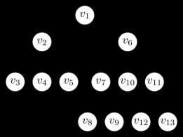
For a tree �� and a vertex ��, let ���� be the directed graph whose underlying graph is �� and in ���� each edge is directed in such a way that for each vertex �� ∈��(����) there is a path in ���� from �� to ��. We will say that ���� is a rooted tree with a root ��. Fig. 1 illustrates the rooted tree ����1 with the root ��1.

Let ���� be a rooted tree, the depth of a vertex ��, denoted by ℎ(��), is the length of the unique path from the root �� to the vertex ��. A vertex �� is said to be the parent of the vertex ��, denoted by ��(��), if �� →��. In that case the vertex �� is said to be a child of the vertex ��. The children of a vertex �� ∈��(����) are the set �� ⊆ ��(����) of all vertices �� of the tree ���� satisfying the condition �� →��. A vertex having no children is said to be a leaf vertex. Non-root two vertices ��,�� ∈��(����) are said to be sibling vertices if ��(��) =��(��). For a vertex �� let ��(��) be the subtree induced by all the vertices �� such that there is a path from �� to �� in ���� [1].

Fig. 1. A rooted tree ����1 with the root ��1

A cut vertex is any vertex whose removal increasesthe numberofconnected components. Anyconnected graph decomposes into a tree of biconnected components called the block-cut tree of the graph. A

block graph is a type of graph in which every biconnected component (block) is a clique (every two distinct vertices in the clique are adjacent). Fig. 2 illustrates an example of a block graph and its respective block-cut tree.

Fig. 2. Block graph on the left and its respective block-cut tree on the right. Even block graphs are a subclass of block graphs where each block has an even number of vertices.

Fig. 3. An example of an even block graph. Each block is a clique with an even number of vertices.

An edge-coloring of a graph �� is an assignment of colors to the edges of the graph so that no two adjacent edges have the same color. An edge-coloring of a graph �� with colors 1, ,�� is an interval t-coloring if all colors are used, and the colors of edges incident to each vertex of �� form an interval of integers. A graph �� is interval colorable if it has an interval t-coloring for some positive integer ��. The set of all interval colorable graphs is denoted by ��. The concept of an interval edge-coloring of a graph was introduced by Asratian and Kamalian [2]. This means that an interval t-coloring is a function ��:��(��)→{1,…,��} such that for each edge �� the color ��(��) of that edge is an integer from 1 to ��, for each color from 1 to �� there is an edge with that color and for each vertex �� all the edges incident to �� have different colors forming an interval of integers. The set of integers {��,��+1, ,��}, �� ≤��, is denoted by [��,��]. Let ���� be the set [1,��] of integers, then 2���� is the set of all the subsets of ���� We will denote by ��(����) the set of all the elements from 2���� that are an interval of integers. More formally ��(����)={��:�� ∈ 2����,������������������������������������������������������������}

For an interval coloring, �� and a vertex ��, the set of all the colors of the incident edges of �� is called the spectrum of that vertex in �� and is denoted by ����(��)

The smallest and the largest numbers in ����(��) are denoted by ����(��) and ����(��), respectively.

Interval edge-colorings have been intensively studied in different papers. In [3] it was shown that every tree is from ��. Lower and upper bounds on the number of colors in interval edge-colorings were provided in[4] and the bounds were improved for different graphs: planar graphs [5], r-regular graphs with at least 2⋅��+2 vertices [6], cycles, trees, complete bipartite graphs [3], n-dimensional cubes [7,8], complete graphs [9, 10], Harary graphs [11], complete k-partite graphs [12]. In [13], interval edge-colorings with restrictions were considered, in which case there can be restrictions on the edges for the allowed colors.

Interval edge-coloring of even block graphs Here we consider the following two problems for even block graphs.

Problem 1: Interval edge-coloring

Given a graph ��. Find any interval edge-coloring. More formally, find an edge-coloring ��:��(��)→ ℕ such that for each vertex �� all the edges incident to �� have different colors forming an interval of integers.

Problem 2: Interval edge-coloring with minimal colors

Given a graph ��. Find the minimal �� for which there is an interval t-coloring. More formally, find an

edge-coloring ��:��(��) →[1,��] (with minimal ��)such that for each color from 1 to ��, there is anedge withthat color, and for each vertex �� all the edges incident to �� have different colors forming an interval of integers.

First, we will solve the Problem 1 for even block graphs byprovidingan upper bound for ��(��).Then we will show that the upper bound can not be improved. This way, we will get close to the solution of the Problem 2 for even block graphs.

It is known that all trees have interval edge-coloring. A complete graph ���� has an interval edge-coloring if and only if �� is even. The class of even block graphs contains the class ofeven complete graphs and the class of trees (since every block in a tree is an edge and contains two vertices). Let us first show how to color the edges of a complete graph to have an interval edge coloring.

Lemma 1: For a complete graph ��2 ��, and for any positive integers ��,�� with �� ≤�� and �� ��+1=2⋅

�� 1, there is an interval edge-coloring �� such that ����(��) =[��,��] for all �� ∈��(��2 ��) Let �� =2⋅��. From [4] it is known that ��(��2��)=2⋅�� 1=Δ(��2��). It means there is an interval t-coloring with �� =2⋅�� 1. Adding �� 1 to all the edges of an interval t-coloring will produce an interval edge-coloring with colors from �� to ��+ (2 �� 1) 1=��. When it comes to the coloring, assume the vertices are labeled from 1 to ��. Coloring the edge (��,��),1≤��,�� ≤�� with the color ��+((��+ ��)%(�� 1) will ensure that all the spectrums are [��,��] ∎

Unlike complete graphs, it is not true that if a block graphhas a block withan odd number ofvertices, then it does not have interval edge-coloring. Fig. 4 illustrates such a counterexample.

Fig. 4. An example of a block graph that has interval edge-coloring.

We will show that every even block graph has an interval edge-coloring.

Theorem 1: Every even block graph �� has an interval edge-coloring. Furthermore ��(��) ≤2⋅ (Δ(��) 1) when Δ(��) ≥2

If the graph �� is a complete graph with an even number of vertices, then from Lemma 1 ��(��) =Δ(��) When Δ(��)≥2, 2 (Δ(��) 1)≥Δ(��) hence the statement is valid.

We can assume that �� is not a complete graph. It means the graph �� has at least one cut vertex. Let �� = 2⋅(Δ(��) 1). Let �� be an arbitrary cut vertex and consider the rootedblock-cut tree ���� ofthe graph ��. We will provide a top-down approach for coloring the graph edges. For the cut vertices of the block-cut tree, we will color the edges of that vertex and all the blocks to which it belongs. Every block �� of the graph �� will be colored with some [��,��] interval �� ��+1= |��(��)| 1. Since all the blocks have even number of vertices, from Lemma 1 it is possible to have such interval edge-coloring. At every point, the colored edges will form an interval of integers for every vertex (even if some of the edges for that vertex are not colored yet). For a block vertex �� ∈��(����), let ��(��) be the block of the graph ��

For the vertex �� we can color its incident edges with the colors from 1 to ����(��). Let ��1,…,���� (�� = ������(��)) be the child vertices of �� in ����. Since �� is a cut vertex, ��(��1), ,��(����) are the blocks containing the vertex ��. Let ���� =|��(��(����))| 1 for 1≤�� ≤��. If we color the block ��(��1) with colors [1,��1], the block ��(��2) with colors [��1 +1,��1 +��2], … , the block

��(����) with colors [��1 +��2 + +���� 1 +1,��1 +��2 + +����] using the Lemma 1 then the spectrum of the vertex �� will be the interval [1,����(��)] and all the block that contain the vertex �� will have an interval edge-coloring.

Now consider any non-root vertex �� ∈��(����). The vertex �� is either a cut vertex or a block vertex in ����.

Ifthe vertex �� is a cut vertex, then its parent vertex ��(��) is a block vertex. Since we already colored the edges of the block ��(��(��)), the colors of the edges incident to �� that belong to that block form an interval of integers. The length of the interval is equal to �� = |��(��(��(��)))| 1 and assume it is the interval [��,��],(�� ��+1=��,[��,��]⊆[1,��]. Since �� is a cut vertex, it belongs to more than one block, which means it has edges that do not belong to the block ��(��(��)), hence 1≤�� ≤Δ(��) 1

Nowwe needtocolortherest oftheedgesincident to �� so that each of the blocks that contain the vertex �� are colored with intervals. Let ��1, ,���� be the child vertices of �� and let ��(��1), ,��(����) be their respective blocks. Let ���� =|��(��(����))| 1 whichis the number ofedges fromthe block ��(����) incident to the vertex ��. Let �� =∑ ���� �� ��=1 then ��+�� =|��(��(��(��)))| 1+ ∑ (|��(��(����))| 1) �� ��=1 =����(��) ≤Δ(��) Assume that we can find an interval [��,��]⊆[1,��] of length �� such [��,��]∩[��,��]=∅ and [��,��]∪[��,��]∈ ��(����). Then the vertex �� would be colored with interval of integers and we could take the interval [��,��] and splititintosmallerintervals oflengths ��1, ,���� tocolor

the blocks correspondingto the children of ��. Usingthe Lemma 1, the block ��(��1)could be colored with colors [��,��+��1 1], the block ��(��2) with colors [��+ ��1,��+��1 +��2 1], , the block ��(����) with colors [��+��1 +⋯+���� 1,��+��1 ⋯+���� 1]=[�� ���� + 1,��] since �� =∑ ���� �� ��=1

Now let us show that we can always find such [��,��] interval. If �� �� ≥1 then [��,��]=[�� ��,�� 1] If �� ≤�� we need to show that ��+�� ≤�� in which case we could take [��,��]=[��+1,��+��]. Since 1≤�� ≤ Δ(��) 1 and ��+�� ≤Δ(��) we have 1≤�� ≤Δ(��) 1

��+�� =��+�� 1+�� ≤��+�� 1+�� and we know that ��+�� ≤Δ(��), �� ≤Δ(��) 1 we can get ��+�� 1+�� ≤Δ(��) 1+Δ(��) 1=��.

The intuition is that as long as �� is greater or equal than 2⋅(�� 1)+��+1 we canalways findaninterval of length �� to the left or the right of any given interval that has length ��. The maximal value will be achieved if �� =1,�� =Δ(��) 1 in which case we get 2 (Δ(��) 2)+2

If the vertex �� is a block vertex, then we already knowhowtheedgesoftheblock��(��)arecoloredsince the parent vertex ��(��) is a cut vertex. Using the fact that ��(��) has even number of vertices and is a clique we colored with some colors [��,��] such that �� ��+ 1=|��(��(��))| 1 using the Lemma 1. We can continue coloring the children cut vertices of the vertex ��. ∎

Theorem 2. For every even integer �� there exist an even block graph �� withΔ(��)= �� forwhich (��) ≥ 2 (�� 1)

Let �� =2 �� beaneveninteger.When �� =2we have 2 (�� 1)=2=�� and since we should have Δ(��)=�� and it is known that ��(��)≥Δ(��) the statement is obvious for this case. We can assume �� ≥4 in which case 2 (�� 2)+1≥��+1

We need to construct an even block graph �� such that Δ(��)=�� and there is no interval edge-color with 2⋅(�� 2)+1 colors. Consider the graph illustrated in Fig. 5.

Fig. 5. An even block graph where the vertex �� is connected to the vertices ��1, ,����. Each of the vertices ��1 ,���� are inside blocks that are cliques having �� vertices.

In that graph, there is a root vertex �� that is connected to �� vertices ��1,…,���� and each of these �� vertices belongto a clique ���� each of which has �� vertices. The constructed graph has ��2 +1 vertices. Let �� =2⋅ (�� 2)+1 and suppose there is an interval edge-coloring �� such that all the colors are from 1 to ��. The colors of the edges (��,��1), ,(��,����) form an interval of integers [��,��] with length �� (�� ��+1=��).

Consider the color �� 1 which is the middle color of the interval [1,��]. Since [��,��]⊆[1,��] (�� ≥ ��+1) it means �� ≥�� and �� ≤�� ��+1=�� 2

which means the color �� 1∈[��,��]. Let ���� be the vertex for which ��(��,����)=�� 1 and consider the clique ���� that contains the vertex ����. If we take the edges of the clique that have color �� 1, they will form a matching and will not contain the vertex ����, since it is already connected to the vertex �� with the color �� 1. Since |��(����)|=�� =2⋅�� there is a vertex �� ∈��(����) which does not have an incident edge with color �� 1 Fig. 6 illustrates that case.

Fig. 6. The edges of a clique containing the vertex ���� having color �� 1. There is a vertex �� that does not have an incident edge with color �� 1

For the vertex ��, ����(��)=�� 1 and the spectrum ����(��)=[��,��] has length �� 1 (�� ��+1= �� 1). This means that either �� ≥�� or �� ≤�� 2 If �� ≥�� then �� ≥��+(�� 1) 1=2 (�� 1)≥ ��+1 which is a contradiction. If �� ≤�� 2 then �� ≤ �� (�� 1)+1=0 which is a contradiction. This means there is no interval edge-coloring with �� =2 (�� 2)+1 colors hence ��(��)≥2 (�� 1) ∎

Corollary: If �� is an even block graph then ��(��)≤2⋅(Δ(G) 1) and the inequality can not be improved for the class of even block graphs.

REFERENCES:

1. West D.B. Introduction to Graph Theory. Prentice-Hall, New Jersey, 1996.

2. Asratian A.S., Kamalian R.R. Interval Colorings of Edges of a Multigraph. Appl. Math. 5 (1987), 25 34 (in Russian).

3. Kamalian R.R. Interval Colorings of Complete Bipartite Graphs and Trees. Preprint of the Computing Centre of the Academy of Sciences of Armenia Yer. (1989).

4. Kamalian R.R. Interval Edge-colorings of Graphs Doctoral Thesis. Novosibirsk (1990).

5. Axenovich M.A. On interval colorings of planar graphs. Congr. Numer. 159 (2002) 77–94.

6. Kamalian R.R., Petrosyan P.A. A note on interval edge-colorings of graphs. Math. Probl. Comput. Sci. 36 (2012) 13–16.

7. Petrosyan P.A. Interval edge-colorings of complete graphs and n-dimensional cubes. Discrete Math. 310 (2010) 1580–1587. https://doi.org/10.1016/j.disc.2010.02.001

8. Petrosyan P.A., Khachatrian H.H., Tananyan H.G. Interval edge-colorings of Cartesian products of graphs I. Discuss. Math. Graph Theory 33 (2013) 613–632. https://doi.org/10.7151/dmgt.1693

9. Khachatrian H. H., Petrosyan P. A. Interval edge-colorings of complete graphs. Discrete Mathematics, 339(9), (2016) 2249–2262. https://doi.org/10.1016/j.disc.2016.04.002

10. Kamalian R. R., Petrosyan, P. A. On Lower Bound for W(K2n) Mathematical Problems of Computer Science, Vol. 23, (2004), pp. 127 129

11. Kamalian R.R., Petrosyan P.A., On interval edge colorings of Harary graphs H2n 2,2n Mathematical Problems of Computer Science, Vol. 24, (2005), pp. 86-88

12. Kamalian R. R., Petrosyan P. A. On Interval Colorings of Complete k-partite Graphs Kn k . Mathematical Problems of Computer Science, Vol. 26, (2006), pp. 28 32

13. Sahakyan A. K., Kamalian R. R. (2021). INTERVAL EDGE-COLORINGS OF TREES WITH RESTRICTIONS ON THE EDGES. Proceedings of the YSU A: Physical and Mathematical Sciences, 55(2 (255)), 113-122.

MEDICAL SCIENCES

УДК: 616.71-006; 616.71-018.46-006.441

MODERN METHODS OF DIAGNOSIS OF MALIGNANT LYMPHOMA OF BONES

Aliyeva I., Doctor of philosophy (PhD) in Medicine, Senior teacher of department Cytology, Embryology and Histology; Sultanova T., Doctor of philosophy (PhD) in Medicine, Assistant professor of department Cytology, Embryology and Histology; Aliyarbayova A., Doctor of philosophy (PhD) in Medicine, Assistant of department Cytology, Embryology and Histology; Yildirim L., Assistant of department Cytology, Embryology and Histology; Qurbanova Sh. Assistant of department Cytology, Embryology and Histology; Azerbaijan Medical University, Baku Department of Cytology, Embryology and Histology

Алиева И.О., кандидат мeдицинских наук, старший преподаватель; Султанова Т.А., кандидат мeдицинских наук, доцент; Алиярбекова А.А., кандидат мeдицинских наук, ассистент; Йылдырым Л.Е., ассистент; Курбанова Ш.К. ассистент. Азербайджанский Медицинский Университет, Баку кафедра Цитологии, Эмбриологии и Гистологии DOI: 10.24412/3453-9875-2021-70-1-31-35

Abstract

The problem of combating bone tumors is currently one of the most pressing problems in medicine. At present, bone tumors have been clinically and morphologically investigated in sufficient detail, however, interest in their study continues unabated. Malignant bone lymphoma, in contrast to Ewing's sarcoma, is characterized by a relatively slow course and late development of metastases and affects patients mainly over the age of 20 years. The purpose of this study is to timely detect malignant bone lymphoma (reticulosarcoma) with modern methods and prevent lethal consequences. In this work, the research methods made it possible to clarify the location of the formation in the bone that was detected during a clinical study or was not externally determined. The study included 26 patients with malignant bone lymphoma, who are being treated at the cityoncological dispensary named after V.I. A.T. Abbasov (Baku), Research Institute of Traumatology and Orthopedics (Baku) and Federal State Budgetary Institution" N.N. Blokhin National Medical Research Center of Oncology "of the Ministry of Health of Russia, AMU Oncology Clinic from 2008 to 2018. The main clinical, laboratory, radiological characteristics of the tumor, survival rates, and prognosis factors were assessed.

медицине. В настоящее время опухоли костей клинически и морфологически исследованы достаточно подробно, однако не ослабевает интерес к их изучению. Злокачественная лимфома кости, в отличие от саркомы Юинга, характеризуется относительно медленным течением и поздним развитием метастазов и поражает больных преимущественно в возрасте старше 20-ти лет. Цель данного исследования вовремя выявление современными методами злокачественной лимфомы кости (ретикулосаркомы) и предотвращать летальные последствия. В данной работе методы исследования позволили уточнить расположение в кости образования, выявленного при клиническом исследовании или внешне не определяемого. В исследование включено 26 пациента со злокачественной лимфомой кости, находящихся на лечении в городском онкологическом диспансере им. А.Т. Аббасова (г. Баку), НИИ Травматологии и Ортопедии (г. Баку) и ФГБУ «НМИЦ онкологии им. Н.Н. Блохина» Минздрава России, онкологической клиники АМУ с 2008 по 2018

г. Оценивались основные клинические, лабораторные, рентгенологические характеристики опухоли, показатели выживаемости, факторы прогноза.

Keywords: tumor, reticulosarcoma, Ewing's sarcoma, histochemistry, immunohistochemistry. Ключевые слова: опухоль, ретикулосаркома, саркома Юинга, гистохимия, иммуногистохимия.

В соответствии с Международной гистологической классификацией опухолей первичная злокачественная лимфома кости относится к костномозговым опухолям [2, 8, 9]. Дифференциальная диагностика опухолей костей с помощью иммуногистохимии основывается на фундаментальных особенностях опухолевого роста, к которым относится сохранение экспрессии функционирующих генов в условиях злокачественной трансформации клетки, [1, 2, 4, 7]. Это проявляется в сходстве фенотипа опухолевыхклеток и их нормальных аналогов. Соответствующие наборы иммуногистохимических признаков имеют костеобразующие и костномозговые опухоли [1, 2, 3,5,6, 10].

ЦЕЛЬ ИССЛЕДОВАНИЯ. Цель данного исследования явилась оценка методом иммуногистохимических исследований клинической значимости выявления компонентов костного матрикса для улучшения и оптимизации диагностики, злокачественных лимфом кости (ретикулосаркомы) МАТЕРИАЛ И МЕТОДЫ ИССЛЕДОВАНИЯ. В настоящую работу в соответствиис поставленнымизадачамивключены данные по комплексному изучению 26-ти больных со злокачественной лимфомой кости, находящихся на лечении в городском онкологическом диспансере им. А.Т. Аббасова (г. Баку), НИИ Травматологии и Ортопедии (г. Баку) и ФГБУ «НМИЦ онкологии им. Н.Н. Блохина»Минздрава России, Онкологической клиники АМУ с 2008 по 2018 год Длярешенияпоставленныхзадачвработеприменялись следующие методы исследований: цитологические, гистологические, гистохимические, иммуногистохимические Клинические методы исследования. На всех 26-ти больных были заведены протоколы, в которые вносили № истории болезни, возраст, пол больных, локализацию патологического процесса, краткий анамнез, клинические и лабораторные данные, № цитологических и гистологических исследований и биопсий, характер проведенной терапии. В нашей работе рентгенологические методы исследования позволили уточнить

уста-

одной

отпечатков, окрашенных гематоксилин-эозином и тионином, с последующей гистологической верификацией диагноза и сопоставлением цитологических и гистологических заключений. В гистологические методы исследования включались случаи, при которых сохранился архивный материал (гистологические препараты, парафиновые блоки или фиксированный в формалине материал), а также текущие наблюдения. Тонкие кусочки кости фиксировали в 10%-ном формалине. После фиксации с целью удаления извести кусочки подвергались специальной обработке - декальцинации 7,5%-ной азотной кислотой. По окончании декальцинации кусочки для предупреждения их дальнейшего набухания и для частичной нейтрализации переносили на 12-24 часа в 5%-ный раствор алюмокалиевых квасцов. Далее обезвоживали в спиртах восходящей концентрации, уплотняли, заливалив парафин исрезытолщиной7-10мкмпосле депарафинизации окрашивали гематоксилин-эозином, пикрофуксином по ван-Гизону и тионином. Материал для гистохимического анализа фиксировался в 80%-ном спирте. Для выявления гликогена использовалась окраска йодной кислотой и реактивом Шиффа (ШИК или PAS-реакция), для выявления хондроида и миксоматозной дегенерации стромы использовалась окраска по Крейбергу. Аргирофильный (ретикулярный) каркас выявлялся с помощью импрегнации серебром, ставилась реакция Перлса на железо и реакция с щелочной фосфатазой на обнаружение остеоидной ткани. Для иммуногистохимического исследованияиспользовалсяматериал,замороженный в жидком азоте, из которого изготавливали криостатные срезы, с последующей фиксации в ацетоне, а также материал парафиновых блоков, фиксированных в 10% формалине. Исследования проводились методом с использованием ферментных иммунных комплексов. Этот тип иммунных комплексов состоит из фермента (антиген) и антител против этого фермента.

(эпифизарное

расположение)

роста, а также центральную (внутри костномозгового канала) или периферическую (интракортикальная, субкортикальная или субпериостальная) локализацию очага, направление роста новообразования, чёткость границ как с окружающей костью, так и с мягкими тканями. Цитологические методы исследования - рутинный цитологический анализ пунктатов, мазков-

Нами в данных исследованиях применён иммуноферментативный авидин-биотиновый метод. Нами в данных исследованиях использовались реактивы фирмы ДАКО (Франция). Все цифровые данные, полученные в ходе экспериментов, подверглись статистической обработке с учётом современных требований. Полученные данные подвергнуты статистической обработке непараметрическими методами по Вилкоксону-Манн-Уитни. Полученные результаты и их обсуждения Для цитологической картины злокачественной лимфомы кости характерно обилие клеток, образующих скопления в виде комплексов или расположенных разрозненно на фоне эритроцитов. Форма

клеток округлая, овальная, полигональная, неправильная. Границы клеток видны не всегда чётко, полиморфизм резко выражен, размеры средние. Цитоплазма скудная или обильная, окрашивается

слабо или резко базофильно, содержит вакуоли. Ядра округлые, иногда овальные, неправильные, располагаются преимущественно в центре клетки (рис.1.).

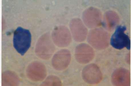
Рис.1. Цитограмма. Форма клеток округлая, овальная, полигональная, неправильная. Окр. Гематоксилин – эозин. Увл.: Об.20, о.10.

Гистологические исследования. Злокачественная лимфома кости макроскопически всегда расположена внутрикостно – в костномозговом пространстве с последующей эрозией или полным разрушением кортикального слоя. В большинстве случаев злокачественная лимфома кости не отличалась чрезвычайно большими размерами или массивными разрастаниями экстраоссального компонента, относительно невысокие темпы роста были характерны для неё. Основной опухолевый узел, разрушая на большем или меньшем протяжении корковый слой, на распиле пораженной кости обычно был расположен в пределах контура кости. Не удавалось установить четкой границы опухоли.

Обычно ткань опухолевого очага имела розовый или серовато-розовый цвет. При злокачественной лимфоме кости патологический перелом довольно часто наблюдался в зоне очага поражения Микроскопические исследования. Опухолевые клетки лимфоидно-ретикулярного и гистиоцитарного типа с большими или меньшими признаками полиморфизма и атипии, с вытянутым или бобовидным ядром и чётко контурированной цитоплазмойявляютсямикроскопическиосновным структурным элементом. Цитоплазматическо-ядерные соотношения значительно больше, чем при саркоме Юинга, где они обычно равны 1:2.

Наиболее четким диагностическим признаком злокачественной лимфомы кости является характер ядер её клеток. В наиболее зрелых формах ядро крупное, имеет почкообразную форму, в более молодых клетках оно явно дольчатое (рис.2.). Дольчатость была настолько резко выражена в некоторых клетках, что создавало картину кучки мелких округлых ядер. Иногда, правда, наблюдались двух- или трёхядерные клетки. В большинстве случаев хроматин ядер в виде грубых глыбок неправильной формы, округлые и большие ядрышки, по 1-2 в каждом ядре, но иногда, как и в клетках саркомы Юинга, хроматин распределён по ядру тонко и равномерно. Значительно чаще при злокачественной лимфоме кости, чем при саркоме

Юинга, наблюдаются фигуры митоза. При злокачественной лимфоме кости, по сравнению с саркомой Юинга, клеточный полиморфизм, таким образом, выступает гораздо заметнее. Гистохимические исследования. При импрегнации серебром в злокачественной лимфоме кости, почти постоянно выявлялась богатая сеть ретикулиновых волокон, оплетающих почти каждую клетку. Клетки злокачественной лимфомы кости при гистохимическом исследовании отличались от клеток саркомы Юинга, кроме того, тем, что в цитоплазме гликогена не содержали. Пиронинофильные гранулы выявлялись при окраске по Браше.

3.

реакция. Высокая положительная реакция общим лейкоцитарным антигеном. Иммуногистохимические исследования. При иммунофенотипировании из 12-ти наблюдений злокачественной лимфомы кости обнаружена высокая положительная реакция только с общим лейкоцитарным антигеном (++) (рис.3, табл.1). Таблица 1. Иммуногистохимические параметры злокачественной лимфомы кости. К-во S-100 NSE HBA-71 LCA NF 12 - - - ++Примечание:

характер роста без формирования каких-либо структур, однотипность морфологического строения клеток, слабовыраженные признаки ядерного полиморфизма, пиронинофилия цитоплазмы, ретикулярные волокна вокруг каждой клетки, а также высокая степень позитивности к такому иммуномаркеру как общий лейкоцитарный антиген могут считаться ориентирующими клинико-морфологическими критериями злокачественной лимфомы в отличие от других костномозговых опухолей.

СПИСОК ЛИТЕРАТУРЫ:

1. 1.Ə.T.Əmiraslanov., H.K.Muradov. Dayaq hərəkət orqanları şişlərində neoplastik angiogenez. Monoqrafiya, Bakı, 2017, 532 səh

2. Мурадов Х.К. Костномозговые опухоли. Монография, Баку, 2002, 174 стр.

3. 3.МурадовХ.К.,Мурадова С.Р.Опроблеме гистогенетического источника развития новообразования скелета. Əziz Əliyevin 120 illik yubileyinə həsr olunmuş elmi konfransın materialları, Bakı 2017, səh. 526-528.

4. Brown R.W. Immunocytochemistry. Clinical cytopathology and aspiration biopsy. New York, 2001,

Norwegian Journal of development of the International Science No 70/2021 35 part 5, p. 535-547.

5. De Rueck J., Sieben G., De Coster W., Roels H. Reticulosarcoma. Histopathology, 2015, vol.4, N2, p. 225-232.

6. Leone A., Costantini A., Guglielmi G. et al. Primary bone tumors and pseudotumors of the lumbosacral spine // Rays. 2011. - Vol. 25. - № 1. -P. 89103.

7. RamziI.Clinicalcytopathologyandaspiration biopsy. Clinical cytopathology and aspiration biopsy.

New York, 2014, part 4, p. 499-511.

8. Pablo P., Fernando MD; López B. Worrisome Juxtacortical Bone Mass. Arch Pathol Lab Med. 2014; May Vol 127: 257-258.

9. Peyruchaud O. [Mechanisms of bone metastasis formation. Soc Biol. 2017; 201(3):229-36.

10. Yamada K., Kudeken W., Muramatsu Y., Sumitomo Sh., Takai Y. Epidemiology of bone cancer. Acta histochem. cytochem., 2015, vol.30, N5-6, p. 477482.

TECHNICAL SCIENCES

RESEARCH OF THE KINETICS OF DRYING OF TYPHA FLUFF DRYING

ProtasovS., Ph.D Engineering, assistant, assistant professor Department of Physical chemistry of materials and production technologies Belarusian State Economic University, Minsk BorovikA., Ph.D Engineering, assistant, assistant professor Department of Physical chemistry of materials and production technologies Belarusian State Economic University, Minsk GorovykhO., Ph.D Engineering, assistant, head of laboratory Minsk City Technopark, LLC «Belspetskomplekt», Minsk Braikova A. PhD in Chemistry, assistant, Head of the Department of Physical chemistry of materials and production technologies Belarusian State Economic University, Minsk ИССЛЕДОВАНИЕ КИНЕТИКИ СУШКИ ПУХА РОГОЗА

ПротасовС. К., к.т.н., доцент, доцент кафедры «Физикохимии материалов и производственных технологий» Белорусского государственного экономического университета, Минск Боровик А.А., к.т.н., доцент, доцент кафедры «Физикохимии материалов и производственных технологий» Белорусского государственного экономического университета, Минск Горовых О.Г., к.т.н., доцент, начальник лаборатории ООО «Белспецкомплект» Минского городского технопарка, Минск Брайкова А.М. к.х.н., доцент, заведующий кафедрой «Физикохимии материалов и производственных технологий» Белорусского государственного экономического университета, Минск DOI: 10.24412/3453-9875-2021-70-1-36-41

Abstract

A diagram of a setup for studying the kinetics of drying typha fluff by weight method according to an improved measurement technique is presented. The curves of drying and curves of the drying rate of typha fluff at different initial moisture content are presented. The conditions for long-term storage of typha fluff have been determined. Аннотация Приведена схема установки для исследования кинетики сушки пуха рогоза весовым способом по усовершенствованной методике измерений. Представлены кривые сушки и кривые скорости сушки пуха рогоза при различном начальном влагосодержании. Определены условия, обеспечивающие длительное хранение пуха рогоза.

Keywords typha fluff, drying kinetics, equilibrium, storage conditions Ключевые слова пух рогоза, кинетика сушки, равновесие, условия хранения. Введение В настоящее

рогозапредлагается использовать

сорбент

проведении работ по ликвидации аварийных разливов нефти и нефтепродуктов на водной поверхности [1]. Рогоз – высшее водное растение, которое растет по берегам водоёмов, на мелководьях, на травяных болотах, а также в разнообразных сырых и мокрых местах: канавах, кюветах, заброшенных карьерах, по обочинам дорог. Стебель рогоза заканчивается цилиндрическим початком темно-бурого цвета. Початок состоит из множества пушинок, которые плотно в нем упакованы. Пушинки расположены вокруг стебля, обеспечивающего их питанием. Сама пушинка состоит из стволика и ворсинок, образующих древовидную структуру. После созревания и

естественной сушки початка пушинки самопроизвольно отделяются от стебля, и рассеиваются в окружающем пространстве. Для использования пуха в качестве сорбента, початки необходимо собрать в период их созревания. В этом случае свежеубранные початки рогоза имеют высокое влагосодержание в пределах 1,4–1,6 кг воды/кг материала, которое способствует развитию микроорганизмов, плесени, грибов и других нежелательных живых объектов, что существенно влияет на качество сорбента. Для длительного хранения пуха необходимо снизить количество влаги до величины, при которой исключается возможность жизнедеятельности плесневых грибов и микроорганизмов. Данные по хранению пуха рогоза в литературных источниках

отсутствуют. Установлено [2], чтобольшинство видов растительного сырья хорошо хранится при влагосодержании 12–15 %. В работе [3] авторы провели исследования по определению равновесного влагосодержания пуха рогоза в помещении с температуройвоздуха19ºCиотносительной влажностью 49 % и установили, что оно составляет 11 %. Это на 1 % меньше минимального влагосодержания для растительного сырья. Таким образом, можно предположить, что для обеспечения длительного хранения пух рогоза необходимо сушить до влагосодержания 0,11 кгвлаги /кгсух.матер Сушку пуха рогоза можно проводить непосредственно в початках, либо после отделения его от стебля. Первоначально проведенные исследования сушки пуха в початках опубликованы в работе [3]. В ней показано, что при конвективной сушке початков до равновесного состояния, требуется ориентировочно восемь часов. Длительность процесса сушки можно объяснить плотной упаковкой пуха в початках. Чтобы это подтвердить, определяли среднюю плотность початка. Длина початка в среднем составляют 0,12 м, а диаметр – 0,025 м.Тогда средний объем одного початка будет равен 5,887·10 5 м3. При средней массе початка 0,05 кг, средняя плотность, которая учитывает массу влаги, стебля и пуха, составит 849 кг/м3. При такой плотности початка, пух в нем должен быть плотно упакован. Отсюда следует, что расстояние между ворсинками пуха тожеочень мало.Для удаления влаги, которая расположена между ворсинками, требуется значительная движущая сила. Она должна преодолеть большое гидравлическое сопротивление, которое препятствует перемещению жидкости в пространстве между плотно расположенными ворсинками.Приотделении пухаот стебля(распушивании початков) ворсинки расправляются, расстояние между ними увеличивается, объем пушинки становится значительно больше. В результате сопротивление выходу влаги из пушинок уменьшается, и время сушки сокращаться. Учитывая эту особенность рогоза, дальнейшие исследования кинетики сушки проводили на пухе, который отделен от стебля. Материалы и методы Основными параметрами, которые влияют на кинетику и время сушки любого дисперсного материала, являются: температура сушки, влагосодержание сушильного агента и скорость его движения через слой материала, влагосодержание материала в начале сушки, толщина его слоя. В отличие от твердых дисперсных материалов (зерно, силикагель), пух, при распушивании початков, существенно увеличивается в объеме, что сказывается на его кажущейся плотности. Отсюда следует, что на кинетику сушки, кроме основных параметров, будет также влиять плотность упаковки пуха в сушилке. Одним из главных параметров сушки является температура проведения процесса. Чем она больше, тем с большей скоростью протекает процесс. Интенсивность сушки также зависит от скорости про-

хождения агента сушки через слой дисперсного материала. С увеличением скорости движения агента через слой время сушки уменьшается. Влияние этих параметров на время и интенсивность сушки пуха приведены авторами в работе [4]. Целью данной работы является определение условий длительного хранения пуха и влияние начального влагосодержания пуха на кинетику сушки. Для определения длительности хранения образцыпуха, высушенныедо влагосодержания11 %, были помещены в матерчатые сетчатые мешки, и в подвешенном состоянии содержались в комнате при температуре 28–20 ºC иотносительной влажности 46–50 %. В течение года регулярно, раз в неделю, определяли влагосодержание образцов пуха. За весь период наблюдений величина влагосодержания пуха колебалась в пределах 11–12 %, а визуально наблюдаемое состояние пуха не изменялось (отсутствовали поражения плесенью, грибами, иными микроорганизмами). Можно сделать вывод, что для длительного хранения пуха рогоза, его необходимо сушить до влагосодержания 11 %. Влияние начального влагосодержания пуха на кинетику сушки проводили при следующих постоянных параметрах: температура воздуха на входе в сушилку 100 ºC; скорость воздуха в сушилке 0,44 м/с; плотность влажного пуха в начале сушки (начальная плотность) 130 кг/м3; высота слоя пуха в сушилке 180 мм. Начальное влагосодержание пуха изменяли в пределах от 0,58 до 1,1 кгвлаги /кгсух.матер Для проведения исследований первоначально определяли влагосодержание пуха перед началом опытов (начальное влагосодержание) Uн. С этой целью брали три образца пуха массой порядка 2 грамм. Измеряли их начальные массы mн с точностью до 0,01 г и сушили в сушильной камере. Периодически образцы вынимали из камеры, и взвешивали.Когдамассаобразцов неизменяласьв течение трех последовательных измерений, принимали ее как массу сухого пуха mсухi. За влагосодержание сухого пуха принимали среднее арифметическое влагосодержания трех образцов. Влагосодержание каждого образца Uнi рассчитывали по формуле (1)

пуха,

сушки проводили методом взвешивания по усовершеноствованной методике замеров. Сущность методики заключается в том, что исследуемая навеска пуха вместе с сушилкойпериодически взвешивали навесахсточностью 0,01 гр. Для этого использовали специальное разъемное устройство, которое позволяло быстро присоединять и отсоединять сушилкуот трубопровода, подводящего сушильный агент. Разность междуобщей массой и массой сушилки позволяла получить массу навески пуха. В результате многократного взвешивания сушимой навески пуха в различные

промежутки времени сушки получали набор значений массы навески и соответствующего ей времени. Влагосодержание пуха в определенное время сушки рассчитывали по формуле (2) Uτ = ��

��сух ��сух , (2) где Uτ – влагосодержание пуха в промежуток времени τ, кгвлаги /кгсух.матер; mn – масса пуха в n – энный промежуток времени, кг; mсух – масса сухого пуха, кг. В результате получали данные изменение влагосодержания пуха в зависимости от времени сушки, на основании которых строили графическую зависимость: влагосодержание материала –

время сушки (кривая сушки). На основе кривой сушки, строилась кривая скорости сушки, а именно зависимость скорости сушки от влагосодержания материала. Эти кривые позволяют определять: продолжительность сушки до равновесного состояния, изменение скорости сушки на протяжении всего времени процесса, величину максимальной скорости сушки. Схема лабораторной установки для исследования кинетики сушки представлена на рис. 1. В качестве сушильного агента использовался подогретый атмосферный воздух. С целью уменьшения потерь теплоты в окружающую среду, сушилку помещали в тепловую изоляцию. 1 – воздуходувка; 2 – прибор для измерения расхода воздуха (ротаметр); 3 – электрический калорифер; 4 – термометр; 5 – корпус сушилки; 6 – опорная решетка; 7 – лабораторный трансформатор; 8 – весы; 9 – крышка сушилки перфорированная; 10 – разъемное устройство. Рисунок 1. – Схема лабораторной установки сушилки Атмосферный воздух подавался воздуходувкой

Температуру воздуха измерялась термометром 4, и регулировалась с помощью лабораторного трансформатора 7. После прогрева установки до необходимой температуры при постоянном расходе воздуха, предварительно взвешенная сушилка с пухом устанавливалась в разъемное устройство 10, и фиксировалось время начала сушки. Подогретый воздух проходил через слой пуха, насыщался влагой, и через отверстия в крышке 9, выходил в атмосферу. Через 3 минуты

сушилка отсоединялась от трубопровода, взвешивалась на весах 8, и снова устанавливалась на рабочее место. Время отсоединения, взвешивания и соединения сушилки с трубопроводом составляло 8–10секунд.Последующиедва взвешивания производились также через 3 минуты. Остальные временныеинтервалымеждуизмерениямимассысушилки увеличивались в зависимости от начальных параметров сушки. Результаты и их обсуждение На рис. 2 представлены кривые сушки при различном начальном влагосодержания пуха.

Используя кривые сушки, определялось время сушки при различном начальном влагосодержании. Графическая зависимость времени сушки пуха от начального влагосодержания

Расчеты показывают, что при увеличении начального влагосодержания в два раза, время сушки пуха увеличивается тоже в два раза. C целью практического применения этих данных, была получена зависимость для расчета времени сушки пуха до равновесного влагосодержания (3)  = 137,83 ��н – 49,99 ��н 2 – 39,12, (3) где  – время сушки, мин; Uн – начальное влагосодержание пуха, кгвлаги /кгсух.матер

0 10 20 30 40 50 60 0 0,2 0,4 0,6 0,8 1 1,2 Соость сушки, 1/с · 10 ^5 Влагосодержание, кг/кг

1 2 3 30

50 0,5 0,6 0,7 0,8 0,9 1 1,1 1,2 Максимальная скорость сушки , 1/с · 10 ^5 Начальное влагосодержание пуха, кг/кг

40

начального влагосодержания пуха максимальная скорость сушки увеличивается. где Nmax – максимальная скорость сушки, 1/с; Uн – начальное влагосодержание пуха, кгвлаги /кгсух.матер. Коэффициент детерминации зависимости (4), R2 =1.

Выводы

1.Для обеспечения длительного хранения пуха рогоза, его влагосодержание не должно превышать 11 %.

2.При увеличении начального влагосодержания пуха рогоза в два раза, время сушки пуха увеличивается в два раза.

3.Сушка пуха осуществляется от максимальной скорости сушки до равновесного влагосодержания во втором периоде сушки. СПИСОК ЛИТЕРАТУРЫ:

1.Горовых О. Г.; Альжанов Б. А. Волоски околоцветника початков рогоза как природный сорбент нефти и нефтепродуктов. /О. Г. Горовых, Б. А. Альжанов // Международный научный журнал «Наука и Мир». № 4 (68), апрель. – Volgograd : 2019. – С. 51–53.

2.Рыкова Л. И., Черняева М. И. Основы микробиологического контроля консервного производства./ Л. И. Рыкова, М. И. Черняева. – М. : Пищевая промышленность, 1967. – 404 с.

3.Протасов С.К., Боровик А.А., Брайкова А.М. Исследование процессов сушки пуха рогоза. / С.К. Протасов, А.А. Боровик, А.М. Брайкова // Мичуринский агрономический вестник. 2021. №1. – С. 87–96.

4.Протасов С.К., Боровик А.А., Горовых О.Г., Альжанов Б.А. Технология сушки отделенных от стебля волосков околоцветника початков рогоза –высокоэффективного нефтесорбента / С.К. Протасов, А.А. Боровик, О.Г. Горовых, Б.А. Альжанов // Slovak international scientific journal. 2021, № 52. –С.24–30.

5.Лыков А.В. Теория сушки. /А.В. Лыков – М. : Энергия, 1968. – 472 с.

№70/2021

Norwegian Journal of development of the International Science ISSN 3453-9875

VOL.1

It was established in November 2016 with support from the Norwegian Academy of Science.

DESCRIPTION

The Scientific journal “Norwegian Journal of development of the International Science” is issued 24 times a year and is a scientific publication on topical problems of science.

Editor in chief – Karin Kristiansen (University of Oslo, Norway)

The assistant of theeditor in chief – Olof Hansen

• James Smith (University of Birmingham, UK)

• Kristian Nilsen (University Centre in Svalbard, Norway)

• Arne Jensen (Norwegian University of Science and Technology, Norway)

• Sander Svein (University of Tromsø, Norway)

• Lena Meyer (University of Gothenburg, Sweden)

• Hans Rasmussen (University of Southern Denmark, Denmark)

• Chantal Girard (ESC Rennes School of Business, France)

• Ann Claes (University of Groningen, Netherlands)

• Ingrid Karlsen (University of Oslo, Norway)

• Terje Gruterson (Norwegian Institute of Public Health, Norway)

• Sander Langfjord (University Hospital, Norway)

• Fredrik Mardosas (Oslo and Akershus University College, Norway)

• Emil Berger (Ministry of Agriculture and Food, Norway)

• Sofie Olsen (BioFokus, Norway)

• Rolf Ulrich Becker (University of Duisburg-Essen, Germany)

• Lutz Jäncke (University of Zürich, Switzerland)

• Elizabeth Davies (University of Glasgow, UK)

• Chan Jiang(Peking University, China) and other independent experts

1000 copies

Norwegian Journal of development of the International Science Iduns gate 4A, 0178, Oslo, Norway email: publish@njd-iscience.com site: http://www.njd-iscience.com