4. Identification strategy

4.1. Treatment assignment

We adopt a Difference-in-Differences (DiD) approach using Callaway and Sant’Anna’s (2021) semi-parametric, staggered, and doubly-robust DiD estimator to infer causality. In essence, this approach helps us obtain a credible estimate of the average treatment effect on the treated (ATT) by comparing outcomes between observationally-comparable COVID-19 SRD grant recipients and non-recipients from before to after the introduction of the grant, after accounting for variation in treatment timing This approach requires two data availability requirements. First, we need data from prior to and after treatment (in this case, the grant) To fulfil this requirement, we make use of five waves of the QLFS from 2020Q1 - 2021Q1 where 2020Q1 serves as the pre-treatment period and most of 2020Q2 through to 2021Q1 as the post-treatment period. 17 Our justification for using these periods is three-fold:

(1) our identification strategy relies on the unique but temporary panel nature of the survey,

(2) considering payments of the grant occurred from the end of May 2020, it is appropriate for 2020Q1 including April and May of 2020Q2 to serve as the pre-treatment period and June in 2020Q2 through to 2021Q1 as the post-treatment period, and

(3) although data from later waves are available, we restrict our post-treatment period to June 2020Q2 to 2021Q1 as this coincides with the first phase of the grant prior to its temporary cessation in April 2021. As such, our analysis and findings are restricted to the first phase of the grant.

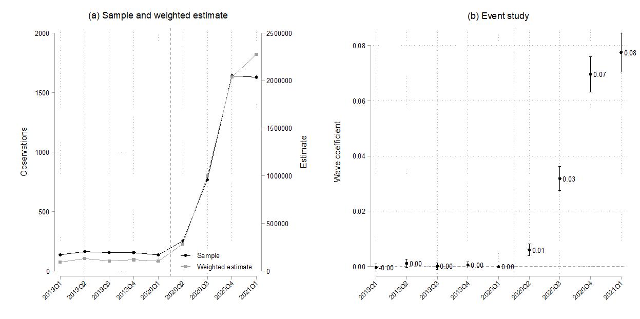
The second data requirement is that sampled individuals need to be categorised into treatment and control groups; that is, recipients and non-recipients of the grant. However, the QLFS survey instrument does not include a question which specifically asks about receipt of the COVID-19 grant, but only the Child Support Grant (CSG), Foster Care Grant (FCG), Old Age Pension (OAP), and Disability Grant (DG) amongst the non-employed. However, the survey does include a question of receipt of ‘other’ welfare grants, which by process of elimination refers to the the War Veteran’s Grant (WVG), Care Dependency Grant (CDG), Grant-in-Aid (GIA), or the COVID-19 grant. As shown in Figure 3, individuals were significantly more likely to be ‘other’ grant recipients in the post-treatment period relative to pre-treatment. In panel (a), which extends the pre-treatment period to one year prior, the number of respondents who answered affirmatively to this question increased substantially from the pre-treatment period (n=150 on average) to the post-treatment period (n=1 073 on average) Indeed, by estimating a linear regression of the binary ‘other’ grant indicator on time fixed effects to obtain (purely descriptive) event study estimates, panel (b) shows that for one year prior to the treatment period individuals were no more likely to be an ‘other’ grant recipient relative to the immediate pre-treatment period of 2020Q1 (the estimates are all close to zero and are not statistically significant), but thereafter this probability increased up to 8 percentage points (a difference which is statistically significant at the 1 percent level). Given that, individually and collectively, the number of WVG, CDG, and GIA recipients was relatively constant during both the pre- and post-treatment periods according to administrative data (see Figure 2 in Section 2.2), the significant uptick in ‘other’ grant recipients in the post-treatment period is arguably due to the variable capturing COVID-19 SRD grant recipients. As such, we make use of this variable, as well as the grant’s eligibility criteria, to indirectly identify recipients of the grant in the post-treatment period. It should additionally be noted that because individuals were only surveyed once per quarter, we are only able to observe receipt once per quarter. Although it is of course possible that recipient individuals received the grant multiple (up to three) times per quarter, due to data availability we are unable to be certain of this.

Source: QLFS 2019Q1 - 2021Q1 (StatsSA, 2019a; 2019b; 2019c; 2019d; 2020a; 2020b; 2020c; 2020d; 2021b).

Authors’ own calculations.

Notes: This figure presents in panel (a) the number of observations and respective weighted population estimates of ‘Other’ social grant recipients as covered in the data over time, and in panel (b) event study estimates on the probability of being an ‘Other’ grant recipient over time relative to the immediate pretreatment period (2020Q1). By process of elimination ‘Other’ includes recipients of the War Veterans’ Grant, the Care Dependency Grant, the Grant in Aid, and from the last month of 2020Q2 the COVID-19 Social Relief of Distress (SRD) Grant. Event study estimates obtained from a linear (OLS) regression of a binary ‘Other’ grant indicator on time fixed effects, weighted using sampling weights and standard errors clustered at the primary sampling unit (PSU) level. Capped spikes represent 95 percent confidence intervals. Vertical line distinguishes the pre-treatment period from the post-treatment period where treatment refers to the introduction of the COVID-19 SRD grant.

Using ‘other’ grant receipt to identify COVID-19 SRD grant recipients in the post-treatment period may however be biased by contamination. Specifically, coding our binary treatment variable equal to one for ‘other’ grant recipients in the post-treatment period would include any possible WVG, CDG, and GIA recipients present in the data. We address this by dropping observations who are eligible for these grants as far as we can identify in the data, 18 however we are not very concerned about such contamination given the very small collective magnitude of recipients.

Recall that individuals were only eligible for the COVID-19 SRD grant if they were between 18-59 years old, unemployed, and were not receiving any other form of government support (i.e. any other social grant or unemployment insurance benefits). Additionally, at the same time as the introduction of the grant, the values of all other existing grants were topped-up. To avoid possibly confounding our estimated effect, we restrict our sample to nonemployed individuals 19 aged 18-59 years who were not receiving any alternative grant or unemployment insurance benefits. Our treatment group comprises individuals who ever reported receipt of the COVID-19 SRD grant (indirectly identified as an ‘other’ grant recipient) in the post-treatment period and our control group comprises those who report nonreceipt . Overall then, our approach compares temporal outcomes of (1) non-employed adults aged 18-59 who neither receive unemployment insurance benefits nor any social grant (control group: n = 48 259 observations in the panel) to (2) non-employed adults aged 18-59 who neither receive unemployment insurance benefits nor any social grant with the exception of the ‘other’ grant (treatment group: n = 3 975 observations in the panel). Described in more detail below, in our modelling we account for variation in duration of receipt among recipients – that is, some recipients received the grant just once and others multiple times

To examine whether the identifying assumption of our DiD approach – that is, in the absence of the grant the trends of the outcomes of recipients would have been similar to nonrecipients on average – we estimate the mean levels of covariates and outcomes by receipt status and period and the corresponding between-group within-period differences as well as the between-group between-period differences. We present these estimates in Table 3. Recall that balanced mean levels of covariates or outcomes by receipt status within each period is not a requirement in a DiD strategy. However what is important is that the difference in the mean levels of a given covariate, but not outcome, by receipt status is constant from before to after the introduction of the grant. The analysis on covariates is equivalent to a placebo falsification test where the DiD model is estimated separately on covariates which theoretically should not be affected by grant receipt, whereas the analysis on outcomes is equivalent to unconditional DiD estimates. We find that in our sample at baseline, relative to non-recipients, recipients are of a statistically similar age and are significantly more likely to be male (which is in line with survey and administrative data (Casale and Shepherd, 2022; Gronbach et al., 2022) as discussed in Section 2) and selfreported African/Black, and less likely to be married, reside in an urban area, and have a tertiary-level education, as shown in the third column. All differences are statistically significant at the 1% level. Following the introduction of the grant, as shown in the secondlast column, the magnitude, direction, and statistical significance of all differences was unchanged, with one exception: Recipients were statistically significantly older than nonrecipients on average; however only marginally by less than one year. It is therefore unsurprising that the between-period differences for all covariates, apart from age, are all close to zero and are statistically insignificant, as shown in the last column. These estimates are in support of the parallel trends assumption and hence the validity of our DiD design. Although the significant estimate on age may be of concern, in the section to follow we describe our adoption of Callaway and Sant’Anna’s doubly robust estimator which accounts for such inter-group temporal differences.

18 WVG recipients are automatically excluded because an individual is only eligible for the grant if they are at least 60 years old (our analysis is restricted to those aged 18 – 59 years). GIA recipients are automatically excluded because an individual is only eligible for the grant if they receive the DG or OPG, who we can identify in the data and exclude from our sample. Unfortunately, given the eligibility criteria of the CDG, we are unable to exclude potential recipients of this grant because the relevant variables (parental status, income, child age, and child disability status) are not available in the data.

19 In any case, grant receipt is only asked of the non-employed in the QLFS, so restricting the sample to this group helps make our treatment and control groups more comparable.

Table 3

Covariate balance by receipt status and period

Source: QLFS 2020Q1 – 2020Q4 and 2021Q1 (StatsSA, 2020a; 2020b; 2020c; 2020d; 2021b). Authors’ own calculations.

Notes: This table presents estimates of mean values for observable covariates for the treatment and control groups accompanied by difference estimates in the periods before and after the COVID-19 SRD grant was introduced. Treatment defined as receipt of the COVID-19 SRD grant (as identified by the ‘other’ grant in the data) in the post-treatment period. Sampling weights employed and standard errors, presented in parentheses, are clustered at the panel (individual) level The magnitude and statistical significance of a given difference are estimated using t-tests. *** p<0.01; ** p<0.05; * p<0.10.

4.2. Model specifications

Before accounting for variation in treatment timing, our model can be described as the following canonical DiD specification for individual ���� in wave ���� which is estimated using Ordinary Least Squares (OLS):

������������ = ����0 + ����1 ���������������� + ����2 �������������������� where ������������ is our binary labour market outcome variable of interest. We are interested in three outcomes in particular: the probability of job search, the probability of reporting trying to start a business, and the probability of ever gaining employment in the post-period Job search is measured through the question “In the last four weeks, were you looking for any kind of work?”, while trying to start a business is through “In the last four weeks, were you trying to start any kind of business?”. Employment is defined as per Statistics South Africa’s conventional definition of working for at least one hour in the reference week or not working because of a temporary absence but still having a job to return to By generating additional outcomes conditional on gaining employment in the post period, we also analyse effect heterogeneity by employment type (wage employment or employee, employer, self- employment, or persons helping unpaid in their household business) and sectoral formality. 20 For each variable, individuals were coded as one if they responded affirmatively and zero if negatively. ���������������� is the binary treatment indicator equal to one for individuals who reported receipt of the COVID-19 SRD grant (indirectly identified as an ‘other’ grant) at least once in the post-treatment period and zero otherwise, and �������������������� is the binary posttreatment indicator equal to one for all observations from June in 2020Q2 to 2021Q1 and zero otherwise. We control for a vector of observable time-varying covariates, ������������ , to reduce residual variance and improve the precision of our estimate, which includes age in years, marital status, a binary urban indicator, highest level of education, and a binary indicator of whether an individual was currently attending an educational institution ������������ is the regression error term. ����3 then represents our coefficient of interest, measuring the estimated average causal effect of COVID-19 SRD grant receipt on our outcome of interest for recipients in the treatment period

However, a recent and emerging econometric literature has shown that when a DiD design has more than two time periods and heterogenous treatment timing (in other words, units are treated at different points in time – a common occurrence in empirical work), estimates obtained from the above canonical specification are often severely biased and do not correspond with interpretable causal parameters (Borusyak and Jaravel, 2017; Athey and Imbens, 2018; Imai et al., 2018; de Chaisemartin and D’Haultfoeuille, 2020; Callaway and Sant’Anna, 2021; Goodman-Bacon, 2021; Sun and Abraham, 2021; Roth et al., 2022). In brief, this is primarily because such models make both ‘clean’ comparisons (between treated and not-yet- treated units) as well as ‘forbidden’ comparisons (between units who are both already-treated but in varying periods) (Roth et al., 2022). Fortunately, a variety of different heterogeneity-robust estimators have been proposed that strictly only use ‘clean’ comparisons to avoid these issues. These estimators often produce similar answers to one another, however the appropriate one depends on the study context. In our study here, while we estimate the conventional ‘problematic’ DiD estimator for comparison, we employ Callaway and Sant’Anna’s (2021) semi-parametric DiD estimator which we believe is most appropriate in our context of multiple time periods and heterogenous treatment timing. The intuition behind this approach is that only never-treated and/or not-yet treated units (i.e. ‘good’ comparisons) should be used as the control group, otherwise estimates will be biased. The key concept behind this approach is the group-time average treatment effect, ������������ (����, ����), where group ���� refers to the time period that treated units are first treated (here, when individuals first receive the COVID-19 SRD grant), defined as follows: ������������(����, ����) = [�������� (����)���� �������� (���� )���� ] where ��������(����)���� is the mean value of the outcome for group ���� at time ���� , and �������� (���� )���� is the mean value of the outcome for the control group ���� (here, individuals who either never received the grant or had not yet received it) at time ���� . The first term then calculates the difference in outcomes at time ���� while the second calculates the difference in outcomes at time ���� 1, which is the period before the first treatment period for group ����. This process then can result in a potentially large number of ������������ (����, ����)’s to consider which may be cumbersome to report, as opposed to the singular ATT in conventional DiD studies However, a particularly attractive feature of the estimator is that it can be used to construct several useful aggregations, including the aggregation of all effects in the post-treatment period for all treatment groups into a singular ATT, the aggregation of such effects for each group ���� (how do effects vary depending on when the grant was received?), and the event study aggregation to study effect dynamics (how do effects vary by length of exposure or number of times the grant was received) 21 We make use of these aggregations in our analysis here.

20 Sectoral formality of employment is defined as per Statistics South Africa’s conventional definition. The formal sector includes workers who are registered for personal income tax, while the informal sector only includes employees who are not registered for personal income tax and work in establishments that employ fewer than five workers, and all other who are not registered for any tax.

Importantly, two other unique features of this estimator are that it does not require strongly balanced panel data, and that it allows for cases where the parallel trends assumption holds either unconditionally or conditionally (that is, only after controlling for a vector of observable characteristics). In the latter case, the estimator allows researchers to flexibly incorporate covariates into the modelling to obtain more comparable treatment and control groups through three alternative estimands: outcome regression (OR) adjustment using OLS; inverse probability weighting (IPW) with stabilised weights, and a doubly robust (DR) estimand based on Sant’Anna and Zhao (2020). While these approaches are equivalent from the identification perspective, they are not from an inference perspective (Callaway and Sant’Anna, 2021). The OR approach requires a correctly specified model of the outcome evolution of the control group, making it explicitly linked with the conventional conditional parallel trends assumption. The IPW approach avoids relying on such a model restriction but instead requires a correctly specified model of the propensity score of individual ���� belonging in group ����, and that they are either in group ���� or an appropriate comparison group. On the other hand, the DR approach combines these approaches and thus relies on modelling both the evolution of the outcome and the propensity score, however it only requires one but not necessarily both to be correctly specified. Therefore, the DR approach is particularly attractive because it relies on less stringent modelling conditions and enjoys additional robustness against model misspecification. As such, although we report both unconditional and conditional results, for the latter we employ the DR estimand using only time-varying covariates (those included in ������������ ) as recommended. We do however re- estimate all conditional models using the other two alternative estimands as a robustness test.

21 It should be noted that the group-time aggregations only allow one to obtain estimates for individuals who first received the grant in 2020Q2, 2020Q3, and 2020Q4 (therefore excluding 2021Q1). Although a subset of individuals in our sample do receive the grant in 2021Q1, we cannot calculate the ������������(����, ����) for these individuals because by the time we reach 2021Q1 this group can only function as a comparison group for the earlier ones.

It should be noted that this approach assumes that treatment is an ‘absorbing state’ In other words, treatment is irreversible: once a unit is treated, they remain treated for the remainder of the panel, such that treatment exposure is ‘weakly increasing’ (it either remains the same or increases). Although there are very few instances in our data where treatment switches on then off again (i.e. individuals report receipt of the grant in one subperiod post-treatment and then not again later), we believe this to be a fair assumption given that it implies individuals do not “forget about their treatment experience” (or grant receipt in this case). An alternative estimator by de Chaisemartin and D’Haultfœuille (2020) does allow for treatment turning on and off, however only subject to a ‘no carryover’ assumption which imposes that potential outcomes only depend on current treatment status and not on full treatment histories (Roth et al., 2022). Given the possibility of dynamic and cumulative effects of grant receipt, we believe this assumption is inappropriate here and thus proceed with Callaway and Sant’Anna’s (2021) approach.

All our model estimates are weighted using sampling weights while our standard errors are clustered at the panel (individual) level and are estimated using a multiplicative wild bootstrap procedure (the mammen approach) with 1 000 replications.

5. Results

In this section we present our estimates of average effects of COVID-19 SRD grant receipt using Callaway and Sant'Anna’s (2021) estimator. We first present the results for our three primary outcomes and thereafter examine effect heterogeneity by employment type and sectoral formality. In each section, we estimate several aggregations described above to examine heterogenous and dynamic effects of grant receipt; specifically, we analyse how effects vary (i) depending on when individuals received the grant and (ii) by ‘treatment exposure’ (in other words, by how long individuals had received the grant for). This latter aggregation also allows us to obtain pre-treatment estimates which can be used to gauge the plausibility of the parallel trends assumption.

5.1. Overall effect estimates

Table 4 presents the aggregated treatment effect estimates. Overall, we find evidence of a highly statistically significant and positive effect of COVID-19 SRD grant receipt on the probability of employment, but only a marginally significant and small effect on trying to start a business and no effect on job search. Regarding employment, our preferred estimate in the top panel of column (6) suggests that receipt of the grant increased employment probabilities by just under 3 percentage points on average, which is quite precisely estimated and is significant at the 1% level. This estimate is marginally lower in magnitude but not statistically significantly different from the unconditional estimate in column (5). The aggregated group-time average treatment effect estimates presented in the bottom panel of the table suggest that this positive effect was driven by those who first received the grant towards the end of 2020: initial receipt in 2020Q2, 2020Q3, and 2020Q4 increased average employment probabilities by 3.7, 5.2, and 7 percentage points, respectively, however the 2020Q2 estimate is only marginally significant at the 10% level The unconditional group-time estimates exhibit a similar pattern. This finding may be attributable to several reasons. For instance, recipients experiencing a greater propensity to engage in job search relative to non-recipients during a period of relatively lower lockdown stringency and greater physical mobility (as discussed by Köhler et al. (forthcoming), the lockdown regulations of earlier periods, such as 2020Q2, prohibited many non-essential activities outside of one’s household). Alternatively, by the end of 2020 and relative to earlier periods, the efficiency of the State’s grant administration system may have increased with a greater amount of time to adjust to the processing and administering of a new grant to a new pool of previously unreached recipients, resulting in higher take-up rates (as implied in Figure 2).

Table 4 Aggregated average treatment effect estimates of COVID-19 SRD grant receipt

Source: QLFS 2020Q1 - 2020Q4 and 2021Q1 (StatsSA, 2020a; 2020b; 2020c; 2020d; 2021b).

Authors’ own calculations.

Notes: This table presents Difference-in-Differences (DiD) estimates of the effect of receipt of the COVID-19 SRD grant on the three primary outcomes of interest All models are estimated using the Callaway and Sant’Anna (2021) DiD estimator, while conditional models are estimated by additionally incorporating Sant’Anna and Zhao’s (2020) doubly robust (DR) estimand. The bottom panel presents the aggregated ATT’s across all periods for each first-treatment cohort. Observations never treated and those not yet treated at the time of treatment used as the control group. Sampling weights employed and standard errors, presented in parentheses, are clustered at the panel (individual) level and are estimated using a multiplicative wild bootstrap procedure (mammen approach) with 1 000 replications. ATT = average treatment effect on the treated. Only time-varying controls included: age, marital status, a binary urban indicator, highest level of education, and a binary indicator of whether an individual was currently attending an educational institution *** p<0.01; ** p<0.05; * p<0.10.

Regarding the probability of trying to start a business, we find only marginal significant evidence of a positive effect. The estimates shown in column (4) suggest that receipt of the grant increased this probability by just 1.2 percentage points, an estimate which is only significant at the 10% level. The aggregated group-time estimates reveal that this effect was driven by individuals who first received the grant in 2020Q3 – the estimate of which is significant at the 5% level The estimates for all other periods are however statistically insignificant. Concerning job search, the magnitude of the overall effect in column (2) is statistically insignificant, in contrast to the significant results from the unconditional model, with one exception: The aggregated group-time estimates reveal a significant (at the 10% level), positive effect of 6 percentage points among individuals who first received the grant in the last quarter of 2020 A comparison of these results to those obtained using the ‘naïve’ models, as presented in Table A1 in the appendix, shows that those in the latter are upwardbiased with respect to job search and trying to start a business and downward-biased with respect to employment, regardless of whether the conditional or unconditional approach is taken. However, as discussed in Section 4.2 and as opposed to our preferred approach, it should be kept in mind that these ‘naïve’ estimates do not have a clear interpretation in the presence of treatment timing heterogeneity (Borusyak and Jaravel, 2017; de Chaisemartin and D’Haultfoeuille, 2020; Callaway and Sant’Anna, 2021; Goodman-Bacon, 2021).

We next examine the dynamics of these estimated effects using Callaway and Sant’Anna’s (2021) event study aggregation. Specifically, we examine effect heterogeneity by length of exposure to treatment (or “duration of receipt”), so effects are estimated and scaled for each period relative to the period first treated using all individuals regardless of when they first received the grant. This aggregation is particularly useful for two reasons: (1) it allows us to analyse beyond the immediate impact of the grant (as discussed by Eyal and Woolard (2011a), heterogeneity in effects by exposure to grants are important to consider as they may speak to them being seen as transitory or permanent income shocks), and (2) it allows us to examine whether grant recipients and non-recipients were statistically similar on outcome dynamics in the pre-treatment period, which we use to gauge the plausibility of the parallel trends assumption.

We find that the effect of COVID-19 SRD grant receipt on employment was initially large but decreased substantially the longer recipients were exposed to the grant. As shown in panels (e) and (f) in Figure 4, we find that mean employment probabilities for recipients and nonrecipients were comparable prior to receipt. The pre-treatment ATT estimates in both the unconditional and conditional models are statistically insignificantly different from zero, which support the plausibility of the parallel trends assumption. Regarding post-treatment dynamics, the “on impact” (at ���� = 0) average effect on employment is close to zero and is statistically insignificant. However being exposed to the grant for one additional quarter raises this effect to 8.6 percentage points – highly significant at the 1% level. Thereafter, the effect dissipates and approaches zero, and after a fourth quarter (or one complete year) of receipt the estimate becomes negative and statistically significant at the 5% level. The unconditional estimates resemble a similar pattern, although the latter estimate remains statistically similar to zero, which may be due to a relatively small subsample of four-period recipients in our data considering the relatively larger confidence interval

Regarding job search effect dynamics, we find that like employment, the “on impact” effect of COVID-19 SRD grant receipt was close to zero and statistically insignificant, however these insignificant effects persisted the longer recipients were exposed to the grant. As shown in panels (a), while the unconditional effect estimate of two quarters of exposure is positive and statistically significant, all others are statistically similar to zero. Similarly, panel (b) shows that the magnitudes of all conditional effect estimates are close to zero and statistically similar to it, including that of the statistically significant unconditional estimate. Regardless of the length of exposure to the grant, these estimates suggest that the grant did not induce job search in the labour market.

Source: QLFS 2020Q1 - 2020Q4 and 2021Q1 (StatsSA, 2020a; 2020b; 2020c; 2020d; 2021b).

Authors’ own calculations.

Notes: This figure presents unconditional and conditional event study estimates of the effect of COVID-19 SRD grant receipt on the three primary outcomes of interest. All models are estimated using the Callaway and Sant’Anna (2021) DiD estimator, while conditional models are estimated by additionally incorporating Sant’Anna and Zhao’s (2020) doubly robust (DR) estimand. ATT's are estimated for each period relative to the period first treated, across all first-treatment cohorts. Here, ‘periods to COVID-19 SRD grant receipt’ indexes the length of exposure to grant receipt. Observations never treated and those not yet treated at the time of treatment used as the control group. Sampling weights employed and standard errors are clustered at the panel (individual) level and are estimated using a multiplicative wild bootstrap procedure (mammen approach) with 1 000 replications. Capped spikes represent 95% confidence intervals.

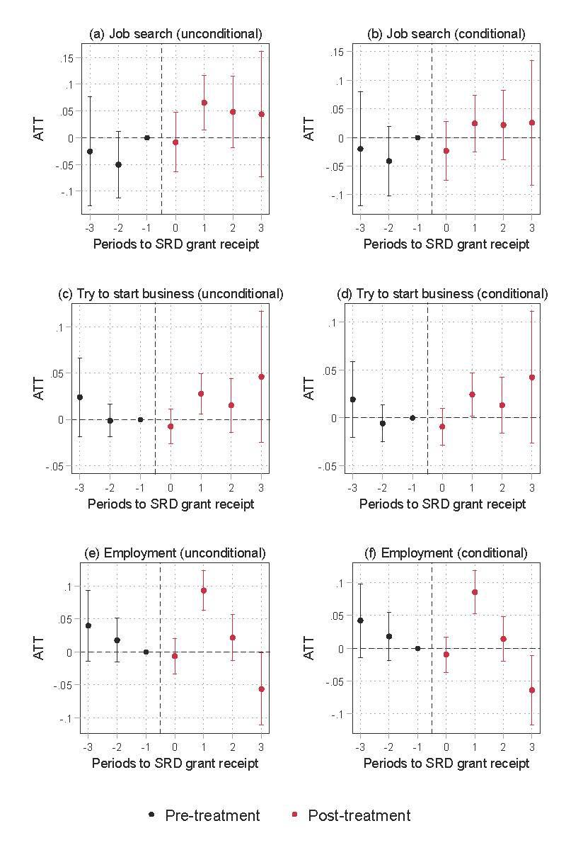
On the other hand, the estimates in panel (d) show that while the “on impact” effect of receipt of the grant on the probability of trying to start a business was, again, statistically insignificant from zero, exposure to the grant for one additional quarter increased this probability by 2.4 percentage points – significant at the 1% level. Estimates for longer periods of grant exposure remain positive and grow in magnitude, however are statistically insignificant. As noted above, may be due to a relatively small subsample of four-period recipients in our data considering the relatively larger confidence interval. As such, we cannot rule out the possibility of larger effects for longer exposure durations. Depending on the validity of such effect dynamics, this finding would then be indicative of larger labour market benefits to receiving the grant for longer periods of time as compared to a once-off receipt, a finding which has been previously documented for other grants in the South African literature (Eyal and Woolard, 2011a).

5.1.1. Effect heterogeneity by employment type

Table 5 presents the aggregated treatment effect estimates by employment type. Overall, we find that the highly statistically significant, positive effect on the probability of employment observed above was driven by a positive effect on the probability of wage employment. As shown in column (2), the results from the conditional model suggest that receipt of the grant increased the average wage employment probability by 2.3 percentage points, statistically significant at the 1% level. The aggregated group-time average treatment effect estimates show that, like the overall employment probability effects, this positive effect was driven by those who first received the grant towards the end of 2020: initial receipt in 2020Q2, 2020Q3, and 2020Q4 increased average wage employment probabilities by 3.1, 4.3, and 5.5 percentage points, respectively. We estimate no statistically significant ATT on the probability of being an employer, as shown in column (4), with the estimate being close to zero in magnitude and statistically insignificant However, we do observe positive and significant albeit relatively small effects among individuals who first received the grant again towards the end of 2020. On the other hand, we do estimate a statistically significant and positive effect on the probability of self-employment, however the effect is relative small (less than 1 percentage point) and only marginally significant. We find no evidence that receipt of the grant had any effect on the probability of engaging in an unpaid household business. As shown in column (8), all estimates in this regard are close to zero in magnitude and statistically insignificant.

Source: QLFS 2020Q1 - 2020Q4 and 2021Q1 (StatsSA, 2020a; 2020b; 2020c; 2020d; 2021b).

Authors’ own calculations.

Notes: This table presents Difference-in-Differences (DiD) estimates on the effect of receipt of the COVID-19 SRD grant on the probability of job search and the probability of trying to start a business, using the Callaway and Sant’Anna (2021) DiD estimator. The bottom panel presents the aggregated ATT’s across all periods for each first-treatment cohort. All models control for individual and time fixed effects. Observations never treated and those not yet treated at the time of treatment used as the control group. Sampling weights employed and standard errors, presented in parentheses, are clustered at the panel (individual) level and are estimated using a multiplicative wild bootstrap procedure (mammen approach) with 1 000 replications. *** p<0.01; ** p<0.05; * p<0.10.

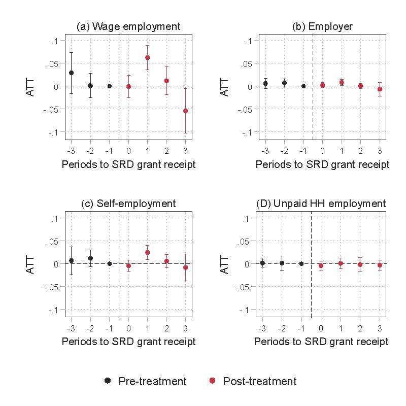
In Figure 5, as before, we analyse the heterogeneity of these estimated effects by employment type by duration of grant receipt, through the use of the event study aggregation. We again find no evidence of an “on impact” effect of receipt of the grant for any outcome; however, after one additional quarter of receipt, we observe a rise in effect estimates for the probabilities of wage employment, self-employment, and becoming an employer. Specifically, as shown in panel (a), one additional quarter of receipt increased the probabilities of wage employment by nearly 6.3 percentage points, significant at the 1% level. This while, as shown in panels (c) and (d), effects on the probabilities of self-employment and becoming an employer were both still significant but notably lower in magnitude at 2.5 and 0.8 percentage points, respectively As before, these effects reduced markedly in magnitude with increased quarters of receipt, with the effect of one full year of receipt on wage employment becoming negative while those on other outcomes remained insignificant. These dynamics closely resemble that of the probability of employment previously observed in Figure 4, which suggests that, even though it is apparent that the overall employment effects were driven by wage employment, effect variation by duration of receipt was largely not a function of employment type Engaging in an unpaid household business serves as the exception for which, as shown in panel (d), we find no evidence of any significant effect by duration of receipt.

Source: QLFS 2020Q1 - 2020Q4 and 2021Q1 (StatsSA, 2020a; 2020b; 2020c; 2020d; 2021b).

Authors’ own calculations.

Notes: This figure presents conditional event study estimates of the effect of COVID-19 SRD grant receipt on employment probabilities by employment type. All models are estimated using the Callaway and Sant’Anna (2021) DiD estimator which additionally incorporate Sant’Anna and Zhao’s (2020) doubly robust (DR) estimand. ATT's are estimated for each period relative to the period first treated, across all firsttreatment cohorts. Here, ‘periods to COVID-19 SRD grant receipt’ indexes the length of exposure to grant receipt. Observations never treated and those not yet treated at the time of treatment used as the control group. Sampling weights employed and standard errors are clustered at the panel (individual) level and are estimated using a multiplicative wild bootstrap procedure (mammen approach) with 1 000 replications. Capped spikes represent 95% confidence intervals.

5.1.2. Effect heterogeneity by employment formality

Table 6 presents the aggregated treatment effect estimates by sectoral formality of employment. Overall, we find that the highly statistically significant, positive effect on the probability of employment observed earlier was driven by a positive effect on the probability of formal sector employment. As shown in column (2), we estimate that receipt of the grant increased the average formal sector employment probability by 2.2 percentage points, significant at the 1% level. As before, we observe that this effect appears driven by individuals who first received the grant towards the end of 2020. The estimates obtained from the equivalent unconditional model, as shown in column (1), are not statistically significantly different from their conditional counterparts. We do not find any strong evidence of any effect on the probability of informal sector employment. In both columns (3) and (4), the effect estimates are close to zero in magnitude and are statistically insignificant. However, we do observe a positive and significant effect of 3.1 percentage points among individuals who first received the grant in the last quarter of 2020. Despite the significance of this latter estimate, its magnitude is 40% lower than the formal sector equivalent in column (2).

Source: QLFS 2020Q1 - 2020Q4 and 2021Q1 (StatsSA, 2020a; 2020b; 2020c; 2020d; 2021b).

Authors’ own calculations.

Notes: This table presents Difference-in-Differences (DiD) estimates of the effect of receipt of the COVID-19 SRD grant on the probabilities of formal or informal sector employment. All models are estimated using the Callaway and Sant’Anna (2021) DiD estimator, while conditional models are estimated by additionally incorporating Sant’Anna and Zhao’s (2020) doubly robust (DR) estimand. The bottom panel presents the aggregated ATT’s across all periods for each first-treatment cohort. Observations never treated and those not yet treated at the time of treatment used as the control group. Sampling weights employed and standard errors, presented in parentheses, are clustered at the panel (individual) level and are estimated using a multiplicative wild bootstrap procedure (mammen approach) with 1 000 replications. ATT = average treatment effect on the treated. Only time-varying controls included: age, marital status, a binary urban indicator, highest level of education, and a binary indicator of whether an individual was currently attending an educational institution. *** p<0.01; ** p<0.05; * p<0.10.

As before, we analyse the heterogeneity of these estimated effects by employment sectoral formality by duration of grant receipt through the use of the event study aggregation in Figure 6. We again find no statistically significant evidence of an “on impact” effect of receipt of the grant for any of the two outcomes; however, it is notable that the sign of the formal sector estimate is positive while that of the informal sector estimate is negative. The latter estimate is marginally significant at the 10% level. Apart from this difference, the dynamics for both outcomes largely resemble one another and that of overall employment probabilities After one additional quarter of receipt, the effect estimates rise to approximately 4.8 and 3.8 percentage points for formal and informal sector employment probabilities, respectively. Thereafter, with additional periods of receipt both effect estimates reduce to become negative in magnitude and marginally significant at the 10% level after one full year of receipt. These dynamics closely resemble that of the probability of employment previously observed in Figure 4. This suggests that, as before, effect variation by duration of receipt was largely not a function of employment formality

Figure 6 Event study treatment effect estimates of COVID-19 SRD grant receipt, by employment sectoral formality

Source: QLFS 2020Q1 - 2020Q4 and 2021Q1 (StatsSA, 2020a; 2020b; 2020c; 2020d; 2021b).

Authors’ own calculations.

Notes: This figure presents conditional event study estimates of the effect of COVID-19 SRD grant receipt on employment probabilities by employment formality. All models are estimated using the Callaway and Sant’Anna (2021) DiD estimator which additionally incorporate Sant’Anna and Zhao’s (2020) doubly robust (DR) estimand. ATT's are estimated for each period relative to the period first treated, across all first-treatment cohorts. Here, ‘periods to COVID-19 SRD grant receipt’ indexes the length of exposure to grant receipt. Observations never treated and those not yet treated at the time of treatment used as the control group. Sampling weights employed and standard errors are clustered at the panel (individual) level and are estimated using a multiplicative wild bootstrap procedure (mammen approach) with 1.000 replications. Capped spikes represent 95% confidence intervals.