Circuit urgery by Ian Bell

Circuit Surgery

Regular clinic by Ian Bell

Transformers and LTspice – Part 1

This month, we will look at the circuits, they can change voltage levels and basics of transformers and some they change they effective impedance of aspects of simulating transformer a load connected via a transformer rather circuits in LTspice. than directly.

A transformer is a passive electronic device that transfers electrical energy, in the form of alternating current, from one circuit to another without using an electrically conductive connection. A transformer comprises two or more coils (looped conductors) in close physical proximity, one of which is used for the energy/signal input (called the primary winding). This coil creates an alternating magnetic fi eld which, by virtual of their closeness, passes through the other coil(s) (the secondary winding(s)), producing a voltage across these windings, which will cause current to fl ow if they are connected to a load.

Transformers come in a very wide range of formats, from tiny surfacemount RF devices to the huge (size of a house) power transformers used in national electrical distribution networks. In between are the transformers used in linear and switched-mode power supplies, pulse transformers used in communications, audio transformers and many other specialist types. The key properties of transformers are that they provide electrical isolation between

Magnetic flux

Changing current

Primary Induced voltage

Secondary

Fig.1. Basic transformer: two coils linked by magnetic fl ux. Fig.2. Transformer with core – this is much more effi cient than the transformer in Fig.1.

Simulation fi les

Most, but not every month, LTSpice is used to support descriptions and analysis in Circuit Surgery. The examples and fi les are available for download from the PE website. Electromagnetic induction

Electric current (DC or AC) creates a magnetic fi eld around a wire. If the wire is wound in a loop the fi eld in the centre of the loop is more concentrated. The fundamental physics of the transformer is called ‘electromagnetic induction’ and was discovered by Michael Faraday and Joseph Henry in the 1830s (for which they were honoured by having important SI units named after them – the farad and henry). Electromagnetic induction is the creation of electromotive force (‘emf’, measured in volts) across an electrical conductor by a changing magnetic fi eld. In a transformer, a changing current in one conductor creates a changing magnetic fi eld which induces an emf in another conductor. A changing magnetic fi eld is required for electromagnetic induction, so although a steady (DC) current creates a magnetic fi eld, AC is required for transformer operation.

Electromotive force

Electromotive force is not a mechanical force – it is the electrical action produced by a non-electrical energy source (eg, c h e m i c a l e n e r g y f r o m a b a t t e r y o r t h e e l e c t r o m a g n e t i c i n d u c t i o n i n a transformer). It drives current to fl ow in a conducting circuit or produces voltage across an open circuit due to the separation of charge. For an open circuit, the charge separation creates an electric fi eld which opposes the separation of charge in balance with the emf driving the separation. The open-circuit voltage is equal to the emf.

Transformer action

Fig.1 shows two coils in close proximity. Applying a varying current to one coil will create the magnetic fi eld, which is visualised as magnetic fl ux lines. Some of the magnetic fl ux will pass through the second coil, resulting in an induced emf (and hence voltage across the coil). Not nearly all of this fl ux passes through the second coil so this arrangement will produce a poor transformer – it will not be effi cient in transferring energy from the secondary to the primary. The situation can be improved by using a transformer core, as shown in Fig.2. If the core material and structure is carefully chosen (particularly its magnetic properties), then the majority of the fl ux will be contained in the core and it will therefore pass through both coils, resulting in an effi cient transformer. In the ideal case 100% of the fl ux is delivered to the second coil.

Transformer circuit symbols usually consist of back-to-back coil/inductor symbols corresponding with the windings. Lines between the coils may be used to indicate the type of core material. Some examples are shown in Fig.3.

Fig.2 indicates the direction of the input current and induced voltage. In order to use the transformer correctly it is often necessary to know which way round the connections are. This is indicated by using dots on the device and on the schematic symbols, known as phasing dots. The dotted terminals have the same instantaneous voltage polarity – when the dotted primary is being driven by the positive half of the AC cycle the dotted secondary will have a positive polarity with respect to the non-dotted terminal.

Magnetic flux

Changing current Core Phasing dot

Induced voltage

Primary: N1 turns Secondary: N2 turns

Air core Ferrite/metal powder core Metal (iron) core

During the positive cycle the current will fl ow into the dotted primary terminal and out of the dotted secondary.

Primary and secondary coil turns

The relationship between the primary and secondary voltage for an ideal transform is determined by the relative number of turns in each winding. Specifi cally, for a primary voltage (vp) applied to a winding with NP turns, and a secondary with NS turns the secondary voltage will be: ����! = ����! ����" ����# ����$ = ����! ����! The secondary voltage is the primary voltage multiplied by the turns ratio. This relationship applies to both the rms and peak values of the voltages. If the turns ratio is larger than 1 then the secondary voltage will be larger than the primary and we have a step-up transformer. The other way round is a step-down transformer. % The latter is commonly used in linear power supply circuits to obtain a low voltage from the mains supply.

A transformer transfers power from primary to secondary. An ideal transformer is 100% effi cient so the input power will equal the output power, for primary and secondary currents (ip and is) we have power vsis = vpip. From the turns equation above, this implies the current in the secondary is: Thus, a step-down transformer will take less current from the primary than is delivered via the secondary. For example, if vp = 240V and vs % = 12V (turns ratio 20:1) and 1A is taken from the secondary the current in the primary will be 50mA (1/20A).

If we connect a resistor (RL) across the secondary, Ohm’s law tells us that vs/is = RL. Using the turns ratio relationships, we get: Where R'L = vp/ip is the effective resistance of the primary as seen by the source driving it. Thus, the transformer has changed the effective value of the load resistor to (Np 2/ Inductors and transformers A coil on its own is an inductor. In fact, a straight wire has inductance, but usually ����! = ����! ����" ����# an inductor component is formed from one or more loops (turns) of insulated wire (sometimes very many turns). The inductance (L) is related to the number of turns squared (N2), but the specific ����! = ����# ����! ����# relationship depends on the type, structure and dimensions of the inductor. In general, we can write L = kN2 so N = √(L/k) for a % given type and size of structure, where k is a constant. For an ideal transformer we = &����! ����#⁄ (����# &����# ����!⁄ (����# = )����! ����# %* )����# ����#* = )����! ����# % %* ����$ & can assume k is the same for the primary and secondary windings, so substituting into the voltage relationship above we get: The turns ratio is equal to the square root of the inductance ratio of the windings (considered as individual inductors). This inductance ratio is important for setting up transformers in SPICE simulations.

Transformers are not simply inductors – the discussion above indicates that an ideal transformer with a resistor connected to the secondary looks like a resistor to the source. The inductance of transformers does matter though, as it affects circuit behaviour and performance. However, it is of less importance in some applications such as mains transformers. If the degree to which the primary and secondary are coupled is not perfect, then the transformer will behave as part transformer and part inductor – this is referred to as leakage inductance. Another important non-ideal characteristic is the resistance of the windings – ideally, this is zero, but wires in real transformers will have some resistance. The many properties of the core are also important in real transformers – one important but complex factor is core saturation, which is a limit on the maximum magnetic fl ux leading to often undesirable outcomes such as waveform distortion. (The one exception to this effect demonstrates Fig.4. Two inductors in LTspice – not a transformer!

Working with LTspice

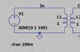
Simulating transformers in LTspice is not as straightforward as other passive c o m p o n e n t s s u c h a s r e s i s t o r s a n d capacitors – we cannot simply drop a transformer symbol onto the schematic. A transformer is made up of two or more coils, so we can draw a transformer symbol by suitably placing two inductors on the schematic, as shown in Fig.4. The symbols can be reflected and rotated using the Ctrl-E and Ctrl-R keys, but it may also be necessary to use the move tool to change the position of the label and value to get the transformer looking right. Fig.4 has a 100Hz, 1V sinewave driving a ‘transformer’ comprising two 1H inductors. The transformer should have a 1:1 ratio, so it should output 1V, but if we simulate this circuit, we will get no output signal, as shown in Fig.5.

The problem is that as far as LTspice is concerned we just have two completely separate coils with no relationship between them. We have to tell LTspice that they form a transformer. This is done by declaring the two inductors to be a mutual inductance, which requires a statement to be placed on the schematic. As you may know, the real input to the simulator is not the schematic drawing but the netlist obtained from it. A netlist is a text description of the circuit plus commands to instruct the simulator what to do. It is generated automatically, but

an advantage of the otherwise weak performance of air-cored inductor – they do not saturate.) ����! = +����# +����! ����⁄ ����⁄ ����# =.����# ����! ����# ����# = Ns 2)RL. If a resistor RL is connected to the .����# ����! ����# secondary of an ideal transformer then the transformer will look like a resistor of value R'L to the source driving the primary. This argument can be applied more generally to impedances (circuits with capacitance and inductance as well as resistance) connected to the secondary. This property of the transformer has uses in impedance matching.

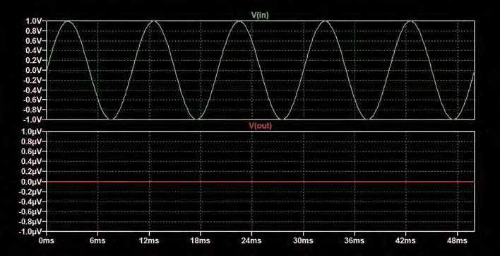
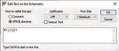
Fig.6. Adding the mutual inductance statement. K x x x L 1 L 2 [ L 3 . . . ] <coefficient>

Fig.7. LTspice transformer circuit. you can view it from the menu using View > Netlist. For Fig.4, the netlist is:

L1 In 0 1 L2 Out 0 1 V1 In 0 SINE(0 1 100) .tran 100m .backanno .end

All of this can be set up via drawing or through menu operations (the . t r a n simulation command is generated via the Edit Simulation Cmd menu item). The .backanno and .end commands are automatically added to every netlist. It should be obvious what .end is for. The .backanno command causes data to be stored that facilitates probing for currents by clicking on schematic symbol pins.

To create a transformer we need to add a mutual inductor component to the netlist, but this cannot be done directly via the menus. We have to add the netlist line for a mutual inductor as text to the schematic. All components start with a specifi c initial letter (L for inductor, V for voltage source and so on). Mutual inductors have initial letter K – the perhaps more obvious M, or T for transformer are already taken by MOSFETs and transmission lines. The syntax of the mutual inductance statement is:

This is a name starting with K, followed by the list of inductors which are coupled together (the windings of the transformer), followed by the coupling coeffi cient. For ideal transformers the coupling coeffi cient is 1, but this parameter can be set in the range 0 to 1 to model transformers where not all of the magnetic flux perfectly links the coils (the non-coupled part forms the leakage inductance). Circuit behaviour can be complex for non-unity coupling coeffi cients, may result in slow simulations, and is often not necessary. It is recommended that simulations are fi rst run with a coupling coeffi cient of 1, even if other values are to be investigated later. For the circuit in Fig.4, we need:

K1 L1 L2 1

To add the mutual inductance statement to the schematic use the Spice Directive (.op) menu item (see Fig.6). Make sure the SPICE directive option is selected (not the comment) or it will not work. Place the text by clicking on the schematic close to the transformer (see Fig.7). Note that once you have added the mutual inductance statement LTspice will automatically add the phasing dots to the schematic – reorientate the inductors if these are not the right way round for how you want your schematic drawn.

Cores and coupling in LTspice

The core lines (see Fig.3) are not part of the LTspice inductor symbol but can be added as additional graphic elements. This should be done using right-click > draw > line, not by drawing a wire. Drawing these as part of the transformer symbol will have no effect on the simulation.

Although we may use an ideal coupling coeffi cient it is usually a good idea to include the winding’s series resistance in the simulation (ideally this is zero but will not be so for a real transformer). This can be measured or obtained from the transformer’s specifi cation. For the circuit in Fig.7, we have added this to the voltage source, which means it can be displayed on the schematic, but this only works because we have a voltage source connected directly to the winding. Series resistance can also be added to the inductor directly by right clicking directly on the inductor symbol. However, this value is not displayed, which could be misleading. It can also be added as a separate resistor, which may in general be the best option.

Simulating the circuit in Fig.7 produces the output shown in Fig.8 – the expected 1V signal.

Fig.9 is the same as Fig.7, except the opposite end of the winding has been grounded (as indicated by the changed position of the phasing dot for L2. The resulting output is 180° (half a sinewave) out of phase with the input (see Fig.10 and compare with Fig.8).

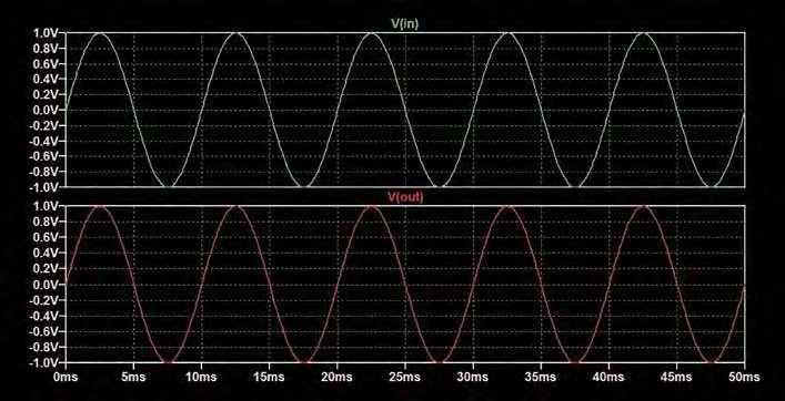
Fig.9. Output phase changed with respect to the circuit in Fig.7.

Inductance values for LTspice transformers

The examples so far have used two equal inductors, so the input and output inductors are equal on the LTspice schematic. As the transformer in LTspice is confi gured from inductors there is no direct way to set the turns ratio – we have to set the ratio of the inductor values to the square of the transformers turns ratio. For example, if we want a step-up transformer with ratio 1:2 then we need an inductor ratio of 1:4. This is shown in the circuit in Fig.11. The resulting waveforms (Fig.12) show a 2V output for a 1V input.

T h i s r a i s e s t h e q u e s t i o n o f w h a t inductance values to use in a real design – these examples just use round numbers for convenience. Obviously, if the inductance values are specifi ed for a real device, then that indicates what to use. Otherwise, if you have a suitable meter (eg, a DC LRC meter) then the value can be measured