SolarShift Turning household water heating systems into MW batteries
FInal report
Turning household water heating systems into MW batteries
February 2025
RACE for Homes
Research Theme : H3 Using home energy technologies for grid support
ISBN: 978-1-922746-68-9
SolarShift
Turning electric water heaters into megawatt batteries
Citations
Yildiz B., Salazar D., Saberi H., Klisser R., Bruce A., and Sproul A. (2024). SolarShift Final Report, H3 Homes RACE for 2030.
Project partners
Acknowledgements
Project team
Collaboration on Energy and Environmental Markets (CEEM), University of New South Wales (UNSW)
• Dr. Baran Yildiz
• Dr. David Saldivia Salazar
• Dr. Hossein Saberi
• Ruby Klisser
• Assoc. Prof. Anna Bruce
• Prof. Alistair Sproul
We would like to acknowledge the following parties for their valuable contributions as part of Industry Reference Group (IRG) members: Endeavour Energy, Ausgrid, Solar Analytics, NSW DCCEEW, Energy Smart Water, Energy Queensland, Origin Energy, AEMC, EDMI, Sustainable Energy Transformation
Acknowledgement of Country
The authors of this report would like to respectfully acknowledge the Traditional Owners of the ancestral lands throughout Australia and their connection to land, sea and community. We recognise their continuing connection to the land, waters, and culture and pay our respects to them, their cultures and to their Elders past, present, and emerging.
What is RACE for 2030?
Reliable, Affordable Clean Energy for 2030 (RACE for 2030) is an innovative cooperative research centre for energy and carbon transition. We were funded with $68.5 million of Commonwealth funds and commitments of $280 million of cash and in-kind contributions from our partners. Our aim is to deliver $3.8 billion of cumulative energy productivity benefits and 20 megatons of cumulative carbon emission savings by 2030. racefor2030.com.au
Disclaimer
The authors have used all due care and skill to ensure the material is accurate as at the date of this report. The authors do not accept any responsibility for any loss that may arise by anyone relying upon its contents.
SolarShift – Turning electric water heaters into megawatt batteries
About Collaboration on Energy and Environmental Markets (CEEM)
The UNSW Collaboration for Energy and Environmental Markets (CEEM) undertakes interdisciplinary research in the design, analysis and performance monitoring of energy and environmental markets and their associated policy frameworks. CEEM’s research focuses on the challenges and opportunities of clean energy transition within market-oriented electricity industries. It does so through collaborations between UNSW researchers from the Faculty of Engineering, the Business School and the Faculty of Arts, Design and Architecture, working alongside Australian and International partners.
CEEM aims for impact through close engagement with energy stakeholders, development of open-source tools and submissions to relevant Australian policy and regulatory processes.
More details of this work can be found at our website. We welcome comments and suggestions and potential collaborations on this research and related tools development, and all our work in this area.
Please feel free to contact Dr. Baran Yildiz at baran.yildiz@unsw.edu.au www.ceem.unsw.edu.au
Executive Summary
Australia is the global leader in per capita rooftop PV system installation as more than 40% of homes own a system with over 25 GW of total installed capacity Rooftop PV offers cheap and clean energy to society however, integration of high levels of rooftop PV has brought challenges such as balancing minimum demand and over-voltage problems experienced in low voltage networks. The existing solutions proposed to manage these issues may be complex and curtail PV generation. This can limit the financial and environmental benefits that can be gained from rooftop PV.
A simpler, yet more effective solution is to use the flexible demand of domestic electric water heaters (DEWH) and shift it to PV generation periods during the day. DEWH includes two main types: resistive (R-DEWH) and heat-pump (HP-DEWH). More than 50% of Australian households have DEWH which makes up a significant demand in the network. DEWH storage tanks offer large thermal storage capacity and can store excess PV generation in thermal energy form. This solution has the potential advantages of reducing power bills for consumers by using low-cost solar energy, reducing PV curtailment in the network and mitigating other challenges associated to integrating higher levels of rooftop PV. Moreover, the penetration of smart meters across houses with PV is close to 100% and across the whole NEM current penetration is around 30% and all households are expected to have a smart meter by 2030. Smart meters provide visibility and can control electrical loads in near real-time. As a result, smart meters are ideal technology to control the flexible demand of DEWH.
Considering this opportunity, RACE for 2030 Project SolarShift has investigated the flexible demand of DEWH from various angles:
• Detailed thermal modelling of DEWH,
• Customer roadmap comparing financial and environmental aspects of different water heating technologies,
• Flexible demand opportunity of DEWH by using real-world operational datasets
• Network impact of flexible DEWH demand
• Forecasting of day-ahead aggregate DEWH demand
The 2-year project has been led by Collaboration on Energy and Environmental Markets (CEEM) research team at University of New South Wales (UNSW) in collaboration with RACE for 2030, Endeavour Energy (EE), Solar Analytics (SolA), NSW Department of Climate Change, Energy, the Environment and Water (DCCEEW), Ausgrid, and Energy Smart Water (ESW). The project has also participated in and contributed to the International Energy Agency (IEA) Solar Heating & Cooling (SHC) Program Task 69, Solar Hot Water.
Thermal modelling
Thermal modelling included annual energy simulations of different DEWH technologies via Transient System Simulation Tool (TRNSYS) and Python programming with the following variables:
Number of people in a household (daily hot water usage),
Hot water draw profiles,
Control strategies, and
Climates across the capital cities of Australia.
Key results are summarized as below:
• Average storage efficiency for DEWH tanks range between 67-72%. This clearly shows that there are significant losses from DEWH tanks and improving the quality of tank and pipe insulation can improve the energy efficiency bringing financial and emissions savings for households.
• Results have shown that reducing this heat loss by half by improving insulation would improve the storage efficiency by around 10%, resulting in annual energy, cost and emissions reduction of 15% However, the improvement of insulation material will also incur additional costs.
• The studied heat pumps with CO2 refrigerants showed average coefficient of performance (COP) ranging between 2.8 and 3.5 for households in Sydney. Our results show that COP is not only influenced by the ambient temperature but also by the water temperature in the tank. COP was greater for the nighttime-controlled load 1 (CL1) and daytime solar-soak control compared to other control scenarios.
• Moving from CL1 to the new Controlled Load 3 (CL3) with additional solar window would see an average increase of 4.2% in total energy consumed due to longer operational window.
• To assess hot water shortage risk against different control strategies and hot water draw profiles (HWDP), Monte-Carlo simulations were carried out. Hot water shortage risk depends on the alignment between heating times and HWDP
• Shifting entire water heating to solar periods may cause risks of hot water shortage for certain HWDP. A potential solution to this is to add a heating window before the early morning consumption.
• Emissions reduce by 67% on average when switching from resistive water heaters to heat pumps.
• The NEM region and energy mix play an important role in emissions. Water heating in Adelaide results in around a third of the emissions compared to the other capital cities such as Sydney, Melbourne and Brisbane that rely on more coal and gas generation.
• Switching from traditional CL1 to an exclusive solar soak control reduces the emissions from ~2.00 tonCO2-eq/yr to 1.65 tonCO2-eq/yr for a 4 people household in Sydney (17% reduction).
• Thermal modelling algorithms are published as an open-source repository code-base in GitHub (tm_solarshift) 1
SolarShift Customer Hot Water Roadmap
Using the thermal modelling results, a Customer Hot Water Roadmap has been developed. The Customer Hot Water Roadmap aims to inform households across Australia of the financial implications of different water heating options including resistive DEWH, heat pump, solar self-consumption through different controlled load strategies, timers or diverters, solar thermal and gas (instantaneous and storage tank). Key findings of the research are summarized below:
• The finances of a hot water system depend on many variables including hot water technology, climate, household size, hot water draw profiles, capital and operational costs, energy tariffs, rebates and incentives (if available), and rooftop PV ownership. Therefore, it is not straightforward to make general recommendations, and each household needs to be considered for their unique case.
• For a base case scenario with 4 people household living in Sydney, household with rooftop PV and a higher cost heat pump set to work with a timer during solar soak hours returns the lowest annual water heating bill.
• For households with resistive DEWH and rooftop PV, utilizing solar generation behind the meter via diverter results in the lowest annual bills closely followed by controlled load options.
1 Repository tm_solarshift, available here
• Lower cost heat-pumps set to work with timers or on a controlled load results in lowest Net-presentcost (NPC) over 10-year period, but typically only have a warranty of 3-5 years. This NPC doesn’t include potential replacement of the lower cost heat-pump.
• The largest NPC component over a ten-year period for resistive DEWH is the annual usage costs, whereas for both the higher cost and lower cost heat pumps and solar thermal heater, it is their initial cost.
• If the daily supply charge is excluded, gas instantaneous systems are cost competitive with resistive DEWH and heat-pumps both for annual bills and NPC. This is mainly because gas energy rates are lower than electricity rates and instantaneous systems have minimal heat losses compared to storage tanks which can lose up to 1/3rd of heating energy.
• It is important to note that gas systems result in significantly higher emissions especially compared to scenarios where rooftop PV is utilized, or grid electricity with a significant proportion of renewable energy generation (i.e. South Australia or Tasmania).
• All payback period cases for upgrading from a R-DEWH to a HP-DEWH or solar thermal falls within each technology’s respective warranty period. Payback period is especially low (<3 years) when moving from R-DEWH to a low-cost heat-pump with an installed capital cost of less than $3,000, when including government rebates and incentives.
• The project team is working on building a public facing online tool where households can use the tool to assist in choosing the most appropriate water heating technology for their unique case.
Real-world data analysis of Endeavour Energy Off-peak Plus Trial
This section focuses on the study of a real-world dataset provided by energy distributor Endeavour Energy (EE) including 12-month of market and power quality (PQ) measurements of ~9,300 households with smart meters across 155 zone substations in New South Wales (NSW). The households DEWH are installed on the controlled load circuit of the smart meters and remotely controlled by the retailers.
• The total DEWH energy throughout the analysed 351 days is around 18,000 MWh and the total shifted load into the daytime is around 5,000 MWh, corresponding to 28% of shifted energy.
• The annual average daily DEWH demand for a household is ~7kWh. During winter months (Jun till Aug) there is an average 4.9 kWh of daily DEWH energy per customer that was shifted into the middle of the day for solar soaking.
• One retailer who had ~37% of the customers with control loads implemented different control strategies throughout the trial, starting with simple static schedules. The retailer switched to more dynamic scheduling of DEWH towards the end of the analysed period considering wholesale market and household DEWH energy consumption. This more dynamic scheduling shifted up to 74% of daily DEWH energy into the daytime, significantly outperforming the rest of the fleet.
• The higher percentage of DEWH shift is promising however, it is important to ensure the household water amenity is not impacted. This needs to be checked and validated by the retailer through customer communications as most DEWH types don’t allow monitoring for temperature and hot water flow
• Taking advantage of lower wholesale prices during the day resulting from higher renewable energy generation, there is considerable wholesale market financial benefits for retailers. According to analysed period, the wholesale benefit is $27/year per household and the proportion of benefits significantly increased towards the later months as the retailer shifted higher percentage of DEWH energy to daytime.
• Currently these benefits are not passed on to households because they can’t access wholesale prices and DEWH is installed on the controlled load circuit of the smart meter preventing solar selfconsumption behind the meter. Retailers should design new tariffs which can pass these benefits onto households by offering much lower rates during high solar generation period.
Impact of flexible DEWH load on the network
This section includes the analysis of PQ data from the EE Off peak Plus Trial as well as undertaking power flow modelling using EE’s low voltage network in NSW.
• Analysis of the real-world power quality data shows small voltage-to-power sensitivity, indicating a high network strength for most of the DEWH customers.
• The median voltage drop associated with DEWH operations was 1.0V considering the entire fleet and the 95th percentile of value drop was 4.8V. 175 smart meters were identified as critical meters which experience voltages above the upper threshold of 253V, which is the 10% allowed deviance from nominal voltage of 230V. For these sites higher voltage-drop values were observed where with the median and 95th percentile values of 1.4V and 7.2V, respectively.
• It was found that customers on several low voltage (LV) networks had highly correlated voltage profiles, indicating potential for utilizing flexible demand of DEWH as a voltage regulation service.
• Analysis of the voltage statistical metrics reveals that for those customers experiencing higher voltages, the operation strategy of the fleet is ineffective. This implies more intelligent location-based controlled load strategies would be of benefit to both network and customers.
• Network modelling using PowerFactory software reveals the potential of DEWH flexible demand in managing LV voltages with different control strategies. Simulation results show that daytime voltages can be further lowered by shifting a higher percentage of DEWH demand shifted to daytime.
• Uptake of heat pump technology may reduce the potential of DEWH load for voltage regulation due to lower power consumption. However, longer operations required by heat-pumps may result in extended smoother voltage reduction profiles.
• Traditional static control schemes are not effective in smoothing aggregated DEWH power due to crude scheduling and randomization which results in intermittent peaks in voltage drops. Smart and location-based DEWH control methods can achieve smoother voltage drop profiles which may be utilized by network in voltage management.
Forecasting of day-ahead aggregate hot water demand
Using various machine learning algorithms, a method was developed by UNSW team based on the available single-year of data The method consists of a hybrid model combining convolutional neural networks (CNN) and long short-term memory (LSTM) networks at two levels of aggregation: the entire DEWH fleet and the zone substation. The developed model uses data from five consecutive days, including total DEWH demand, average dry-bulb temperature, and day of week along with the forecasted average temperature for the next day as inputs, to predict the total DEWH demand for the following day.
• The analysis shows that total daily DEWH demand is highly correlated with average ambient temperature as well as the operating control strategy. In addition, it is observed that regardless of temperature there is a pattern of demand spikes on weekends, where DEWHs experience longer heating windows.
• A lag is observed between DEWH load and temperature changes, which can be attributed to the thermal inertia of DEWH storage tanks. In addition, household behaviours in different times of year also impacts DEWH demand.
• Applying the developed models, the day-ahead DEWH energy demand can be predicted with high accuracy, over 0.95, as measured by coefficient of determination R2.
• Preliminary study of the zone substations with over 117 customers shows promising performance with a mean absolute percentage error (MAPE) of less than 7%.
• Having successful forecasts for day-ahead DEWH demand could be of useful to network operators as well as retailers in managing flexible demand and CER operations.
1 Introduction
1.1 Background
Australia is the global leader in per capita rooftop distributed PV system installation with more than 40% of homes owning a system with an aggregate installed capacity exceeding 25 GW 2. Despite clear financial and environmental advantages, integration of high levels of rooftop PV has also brought challenges. In low voltage (LV) networks, this manifests as minimum demand and over-voltage problems experienced in high-penetration regions, especially in rural parts of the network and towards the end of the feeders 3. The solutions proposed to manage over-voltage issues are inverter power quality response modes, remote export control of PV inverters and charging PV owners for their exports. These solutions can curtail PV power, causing loss of generation and reduced customer revenue.
A simpler, yet more effective solution is to use the flexible demand of domestic electric water heaters (DEWH) and shift it to PV generation periods. It is estimated that more than 50% of Australian households have DEWH such as resistive immersive heaters and heat pumps 4. Most of the DEWHs have 3.6-4.8 kW rated power, which makes up a significant part of the demand in the networks. DEWH storage tanks offer large thermal storage capacity and can store excess PV generation in thermal energy form. This solution has the added advantages of reducing power bills for consumers by using low-cost solar energy and mitigating challenges associated to integrating higher levels of rooftop PV. Considering household batteries are yet to become economically viable, and a great number of households already own a DEWH, utilizing the storage of DEWH can play an important role in the adoption and integration of rooftop PV
Moreover, the penetration of smart meters across the NEM is more than 30% with increasing uptake and all households are expected to have a smart meter by 2030 5. Smart meters provide visibility and control of loads in near real-time. As a result, smart meters are ideal technology to control the flexible demand of DEWH
1.2 Summary of project scope
Project SolarShift has studied the thermal modelling of DEWH, built a customer roadmap for different hot water technologies and investigated the flexible demand opportunity of DEWH by using real-world operational datasets. The 2-year project has been led by Collaboration on Energy and Environmental Markets (CEEM) at University of New South Wales (UNSW) with funding and support from RACE for 2030 and industry partners Endeavour Energy (EE), Solar Analytics (SolA), NSW Department of Climate Change, Energy, the Environment and Water (DCCEEW), Ausgrid and Energy Smart Water (ESW). The project has also participated in and contributed to the International Energy Agency (IEA) Solar Heating & Cooling (SHC) Program Task 69, Solar Hot Water 6
1.2.1 Thermal modelling of DEWH
Thermal modelling of DEWH investigated the thermal performance and heat losses associated with resistive (R-DEWH) system and heat-pump (HP-DEWH) system including their storage efficiency, annual energy
2 Australian PV Institute, Solar PV Status, available here
3 Real-world data analysis of distributed PV and battery energy storage system curtailment in low voltage networks, available here
4 DCCEEW hot water systems, available here
5 AEMC on smart meters, available here
6 IEA Solar Heating and Cooling Programme Task 69 Solar Hot Water, available here
consumption and risks of running out of hot water under different control and hot water use scenarios. Research has also analysed CO2 emissions associated with water heating . Research included a combined method of industry standard thermal modelling software, Transient System Simulation Tool (TRNSYS) 7 in combination with Python programming 8
The simulations were performed considering a base case of a standard 4-people household in Sydney with an average daily hot water consumption of 200 (L/d). The main purpose of the research was to show how DEWH thermal characteristics varied across a range of variables as described below.
Hot water draw profiles (HWDP)
The hot water consumption pattern is modelled with six different hot water draw profiles (HWDP), as defined by previous research 9 : ’morning and evening only’, ’morning and evening with daytime’, ’evenly distributed through the day’, ‘morning dominant’, ‘evening dominant’, and ‘late night’
7 Transient System Simulation Tool (TRNSYS), available here
8 Python, available here
9 Analysis of electricity consumption and thermal storage of domestic electric water heating systems to utilize excess PV generation available, here
Figure 1. Typical hot water draw profiles (HWDP) in Australian households 8
Control strategies
Five different control strategies were studied for the control and scheduling of DEWH. These combinations cover a wide range of possible cases in Australia as shown in the Table 1 below:
Table 1 Studied control strategies for DEWH
Control Type
Abbreviation
General Supply (GS) with flat a GS_flat
General Supply with Time of Use
Controlled Load 1
Controlled Load 2
GS_tou
CL1
CL2
Controlled Load 3
Timer flat (Solar Soak)
Timer time of use (Off-peak)
Diverter ToU (Off-peak)
Diverter + CL1
Other variables
CL3
timer_SS
timer_OP
Diverter_tou
Diverter_CL1
Description
Always connected
Always connected
Overnight – at least 6-hour period between 10 pm and 7 am
24/7 except seasonal peak demand periods - more than 6 hours between 8 pm and 7 am and more than 4 hours between 7 am and 5 pm
CL1 with Solar Soak window between 9am-3pm
Timer control for sunny hours between 9am-3pm aiming for self-consumption
Timer control aiming for off-peak tariff
Diverter for self-consumption with ToU off-peak top up
Hypothetical case (currently not allowed by DNSPs) using diverter for selfconsumption during the day with CL1 tariff for night time heating
Other variables studied for thermal modelling are shown in Table 2 below:
Table 2 Studied variables for thermal modelling
Variable type
Location
Hot Water Draw Profile (HWDP)
Household number of people
PV ownership
Water Heaters
Control Strategies
Tariff options
Variables
Sydney, Melbourne, Brisbane, Adelaide, Canberra
1, 2, 3, 4, 5, 6 (see Figure 1)
2, 3, 4, 5+
Yes - 5kW AC system (PV), No (nPV)
Resistive (R-DEWH), heat pump – high-cost (HPhc), heat pump low-cost (HPlc), solar thermal evacuated tubes with electric boost (STC), gas storage (GStg), gas instantaneous (GI)
Controlled load (CL), general supply (GS), timer, diverter, gas
Flat, ToU, gas
Most of the thermal modelling results presented in this report includes the base case scenario for a household in Sydney with 4 people and HWDP = 1 due to space restrictions. Results for all other scenarios will be made available through SolarShift customer hot water roadmap as described below
1.2.2 SolarShift c ustomer hot water roadmap
Using the outputs of the thermal modelling research, SolarShift customer hot water roadmap investigated the financial viability of water heating for households for a range of different technologies shown in Table 2 The findings reveal the annual bills for each technology under different tariff scenarios, net present value over 10 years, as well as pay-back period for changing across different water heating technologies.
SolarShift project team is building an online tool that will utilize all different simulation and financial results and help households in choosing the best hot water heating technology for their specific case.
1.2.3 Real world data analysis of Endeavour Energy Off P eak P lus
The project analysed real-world operational data from Endeavour Energy’s Off Peak Plus trial in Albion Park, NSW 10 The objective of the research was to investigate DEWH orchestration for a large number of households and find out how much flexible DEWH demand has been shifted to solar generation period via the use of smart meters. Research has also analysed the financial benefits of aggregated DEWH demand control through the use of wholesale market price differences during the solar generation and nighttime.
1.2.4 Network impact of aggregate DEWH orchestration
Through using operational power quality (PQ) data from Endeavour Energy’s fleet, the research has investigated the voltage impact of DEWH orchestration in low voltage networks. Research has focused on the study of real-world power and voltage data as well as undertook network power flow modelling to study different DEWH flexible demand scenarios using DIgSILENT 11 .
1.2.5 Forecasting DEWH network demand
Distribution Network Service Providers (DNSPs), retailers and aggregators may use day-ahead forecast of aggregate DEWH demand in scheduling and optimizing their operations The SolarShift project team has built accurate forecast models for DEWH demand using deep-learning models and historical DEWH demand and climate data.
1.3 Project knowledge sharing
SolarShift has had the following knowledge sharing activities throughout the project:
• Four project milestone and progress reports submitted to RACE for 2030
• Final knowledge sharing report
• Presentation at Australian Energy Market Commission (AEMC) on hot water control and smart meters
• Policy submission to AEMC on the rule change on consumer energy resource (CER) benefits
• Conference presentations: Asia Pacific Solar Research Conference (APSRC 2023), Energy Research Institutes Council for Australia (ERICA) State of Energy Research Conference (2023), Asia Pacific Solar Research Conference (APSRC 2024), IEA SHC Task 69 Meeting (2023 & 2024)
• Media article on Renew Economy 12
• Journal publications (being prepared)
1.4 Structure of the report
This report presents the findings from thermal modelling of DEWH in Section 2. Description and results of the SolarShift customer road map tool is presented in Section 3. Real-world data analysis of aggregated DEWH control is presented in Section 4. Network impact and forecasting of aggregated DEWH demand are presented in Sections 5 and 6, respectively. Report concludes with presenting final discussions and next steps in Section 7.
10 Endeavour Energy Off Peak Plus, available here
11 DIgSILENT, available here
12 Renew Economy Electric hot water is a hero of flexible demand on, available here
2 Thermal modelling of DEWH
2.1 Introduction
One of the main challenges in orchestrating DEWH systems is the uncertainty around the state of charge of the thermal storage tank, making it harder to define optimal heating periods for each customer without impacting their hot water amenity. Thermal simulations provide a better understanding of the expected behaviour of the storage tanks. In this work, the thermal simulations have two main goals:
• First, to study the behavior of the DEWH tank for typical households in Australian capital cities and identify the main variables that affect the performance.
• Secondly, it can be used to provide simulated data for further analyses, such as financial and technoeconomic assessment.
In this section, an analysis of thermal behavior is presented, while the next section shows how these results can be used for financial analysis in creating a road map for a “customer hot water journey” The simulations are developed using an open-source repository built specifically for this project, called “tm_solarshift” 13. It is an object-oriented codebase with a modular philosophy, allowing the definition of different control strategies, weather data source, and import external data, such as market data and energy tariffs. The software was developed to simulate the following types of domestic water heater technologies:
• Resistive immersive (standard heater model Rheem with 3.6 kW nominal power and 315L tank 14),
• Heat pump (Reclaim Model REHP-CO2-315GL with 6.02 nominal COP, 5.22 nominal thermal power, and 315L tank 15),
• Solar thermal (evacuated tubes),
• Gas heater (instantaneous)
• Gas heater (storage)
The codebase also allows simulation of an optional contribution from rooftop PV. Currently, it focuses on two types of analysis: parametric analysis based on annual simulations, and stochastic analysis based on Monte-Carlo simulations.
The results are focused on the DEWH tank’s thermal behaviour under different real-world conditions in Australia. The two main parameters used to characterise the tank’s performance are the storage efficiency and the state of the charge (SOC). The storage efficiency is defined as the thermal energy delivered as hot water over the electricity input, while the SOC is calculated as the useful thermal energy in the tank over the maximum possible stored energy. The presented results mostly use the base case defined in Section 1.2.1.
2.2 DEWH performance analysis
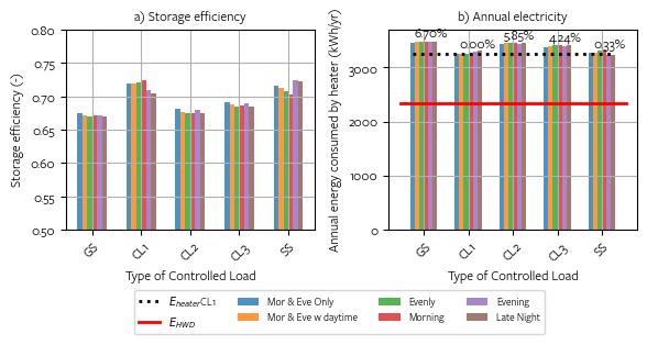
The storage efficiency and the total annual energy consumed by the resistive DEWH are presented for Sydney for different control strategies and HWDP in Figure 2. For each simulation, the volume of annual hot water draw is the kept the same thus, the useful thermal energy delivered to the household is constant in the same environmental conditions. In Figure 2 b), the horizontal red line shows the useful hot water thermal energy. The
13 Repository tm_solarshift, available here
14 Rheem, available here
15 Reclaim Energy, available here.
fraction of the bar above this red line is the thermal losses from DEWH tank to the ambient. Also, for each type of DEWH control strategy, the change in annual energy consumption compared to the base case with CL1, shown as a percentage.
CL1 and solar soak (SS) are the two schedules with better storage efficiency, with an average of 71%. As expected, the longer the electrical circuit is on, the lower the efficiency is. A circuit that is on for longer allows more heating periods, keeping the tank hotter and resulting in higher thermal losses to the environment. In practice, moving from CL1 to the new CL3 would see an average increase of 4.18% of total energy consumed. The results also show that the type of controlled load schedule has a higher influence than the specific HWDP. Similar results were obtained for other cities in Australia, as shown in Appendix D
2.3 State of charge and hot water shortage risk
The ability of the DEWH to provide hot water is represented by the state of charge and is calculated under different hot water use and control strategies. The state of charge (SOC) is an instantaneous variable; thus, its annual distribution provides a ‘picture’ of the tank’s annual behavior. Figure 3 shows violin distribution plots of the SOC distribution for different control strategies. The distribution is influenced by the HWDP; on the left, a highly predicted case (HWDP=1 from Figure 1, only morning and evening), while on the right, a more uncertain profile (HWDP = 3 with water draws throughout the day). Both HWDPs are shown as a small insert on each subplot’s bottom left corner.
As seen, a multi-modal distribution is observed for most of the cases. The first mode is defined by high SOC is due to heating periods associated with the control strategy. The second and third modes depend on the household consumption patterns. Predictable profiles, such as HWDP=1 (Figure 3.a) produce more defined distributions around the modes, meaning that the tank spends longer time in such states. By contrast HWDP=3 creates modes with wider distributions with less predictability. (i.e., HWDP=3, Figure 3.b) A higher HWD predictability could mean more flexibility for tank control, as the tank’s possible states are better known. The
Figure 2. Storage efficiency (left) and annual energy consumed (right) for different HWDP and control loads for the base case. The red line represents the thermal energy consumed as hot water draw, while the percentages are the change in total energy compared with the base case (CL1).
maximum, average, and minimum SOC are shown with blue lines. CL1 and SS have a higher risk of running out of hot water if high-consumption events happen, with minimum SOCs falling as low as 0.22 and 0.25 for SS and CL1, respectively. There is a trade-off between the system’s storage efficiency and reliability, as can be seen when comparing the results from Figure 2 and Figure 3. The system is more efficient when it is discharged deeper, but at the expense of higher risk of hot water shortage.
Figure 3 State of charge (SOC) distribution for different control loads and two different HWDPs. Left: HWPD=1 (morning and evening only, highly predictable). Right: HWDP=3 (evenly distributed, highly uncertain).
The previous analysis poses one of the main questions in this research: what is the optimal control strategy in terms of starting time and duration to minimize the required energy without compromising the provision of hot when it is wanted. To address this question further analysis is performed using Monte-Carlo simulations for specific critical periods of interest. In general, the most challenging period is winter, where the ambient and mains temperatures are lower, the hot water draw is usually higher, and PV generation is at a minimum Therefore, a typical day of July is chosen for these simulations. For each HWDP, timers controlling different starting times and duration are simulated under a sample of 1000 typical days, as shown in Figure 4 The typical days corresponds to synthetic data created using the probability distribution of environmental variables (ambient and mains water temperature), daily hot water draw variability (L/day), and different HWDP. In each case, the hot water shortage risk is estimated as the probability of the tank’s SOC dropping below 10%. The left axis labelled by ‘timer starting’ represents the starting point of heating window for the duration noted on the top of the plots (i.e. ‘Timer on for 5.0 hrs and starting at 10am represents the heating window between 10am –3pm’)
Figure 4. Hot water shortage risk (prob. SOC<10%) for different HWDP and heater timers for a typical day of July in Sydney.
• Hot water shortage risk depends on the alignment between heating times and HWDP as shown by the hot water shortage risk variation across different HWDP
• The hot water shortage risk is reduced when the timer is on for longer, as expected. For 3hrs timer, the risk can reach 22% for when the timer is set to come on at midnight.
• In general, the safer timer windows are those set during the early mornings or late afternoons, regardless of the HWDP.
• For HWDP=1 (Mor & Eve only) the hot water shortage risk is greater especially for timers that start between 10am-12pm where the risk can get as high as 15%, even with long timers (7-9hrs). This because there is less overlap between heating and consumption
• This indicates that shifting entire water heating to solar periods may cause risks of hot water shortage for certain HWDP A potential solution to this is to add a second, shorter heating period, before the early morning consumption.
2.4 Heat pumps simulations
The simulations studied for R-DEWH were also performed for heat pumps. For this project, a Reclaim Energy model (EHPE-4550P-A), with a Coefficient of Performance (COP) of 6.02, heat output of 5.24kW and delivery hot water temperature of 63℃ in design conditions (���������������� = 32 6℃ and ������������������������ = 21 1℃) is modelled 16 This heat-pump model is a split system where the compressor and water storage tank are separate units. Figure 5 shows the main results for heat pumps under the same conditions shown in the previous section. The modelled conditions reflect real-world ambient temperature and inlet water temperature fluctuations throughout the year and are different from the design conditions where the heat-pump’s COP and other specifications are tested for.
16 Reclaim Energy, available here
Figure 5. a) Storage efficiency and b) annual energy consumption for heat pumps. The red line represents the thermal energy consumed as hot water draw, while the shaded section is the electricity consumed by the heat pump. The percentage are the change in total energy compared with the base case (CL1).
In Figure 5 a) the annual energy delivered by the heat-pump tank is shown for the same Sydney base case as presented in Figure 2. In this case, the whole column bar represents the useful thermal energy delivered by the heat pump (same as the resistive immersive DEWH), while the shaded section corresponds to the consumed power by the heat-pump. The ratio between these two variables is the average annual COP, presented in Figure 3b). An average COP ranging between 2.75 and 3.50 is observed. For example, CL1 would be expected to have a lower COP, because the charging periods are at night, where lower ambient temperature is expected. However, CL1 has lower thermal losses and its average hot water temperature is lower too. This means that the heat pump is operating closer to its design point (21.1°C in this case), increasing the COP. The influence of ambient temperature is explored analysing the results in different Australian cities. Figure 6 presents the annual average COP for different control strategies in different cities and for HWDP=3. It is observed a similar COP across different cities, which suggest that location, and by extension, ambient temperature, have a lower impact on the COP, than the control strategy. This suggests that the control strategy is the most influential variable affecting the COP, followed by location and HWD profile
Figure 6. Annual average heat pump's COP for different control strategies in main Australian cities.
2.5 Emissions Analysis
The emissions associated with DEWH usage can be calculated using the emissions of the NEM. This data has 5 minutely temporal resolution and it was imported using an open-source tool, NEMED 17 . When calculating emissions, the NEM region is critical as each state have different energy mix. The simulations are performed on the capital cities of the four major NEM regions and the emission data was applied on each different control strategy Figure 6 shows the results for both resistive heaters (left) and heat pumps (right) for a chosen HWDP=3
The main influence over the total emissions is the DEWH technology and there is a 67% reduction on average when switching from resistive heater to heat pumps. Secondly, the NEM region plays an important role Adelaide with higher renewable energy percentage has significantly less emissions compared to other big cities The control strategy has a lower impact on emissions and the only control strategy with significant reductions compared with the conventional CL1 is solar soak (SS). For example, for Sydney it represents a reduction of 17%, from ~2.0 tonCO2-eq/yr to 1.65 tonCO2-eq/yr.
2.6 Summary
The main conclusions from the thermal analysis can be summarized as below:
• Average storage efficiency for DEWH tanks range between 67-72%. This clearly shows that there are significant losses from DEWH tanks and to the extent that improving the quality of tank and pipe insulation can improve the efficiency and financial and emissions savings could be realised for households. Potentially more stringent thermal efficiency and insulation standards for the DEWH tanks could achieve this
• It is important to note that TRNSYS standard heat loss coefficient (U=1W/m2K) was used in the simulations. When investigated further, reducing this heat loss by half via improving insulation, would improve the storage efficiency around 10% (���������������� = 81% for the base case). This implies a potential annual energy cost and emissions reduction of 15%. However, this requires improvement of insulation
17 National Electricity Market Emissions Data (NEMED), available here
Figure 7. Emissions associated to water heating for four major cities in Australia. a) Resistive heater, b) Heat pumps.
material which has additional costs that also needs to be considered It is important to note that TRNSYS standard heat loss coefficient (U=1W/m2K) was used in the simulations.
• For a given tank storage efficiency, the modelled results show that for most of the studied cases, control strategy has higher impact on overall thermal efficiency than the HWDP. This indicates that external control strategies have great importance in improving energy efficiency of DEWH.
• The best thermal performance is achieved with the controlled load 1 (CL1) and solar soak (SS) control strategies as these have, the least number of hours where DEWH can be operational resulting in lower tank temperature and consequently, lower heat losses to ambient. The efficiency of other controlled load strategies can be improved by decreasing the operational window but this would also increase the risk of hot water shortage
• Increasing the state of charge (SOC) decreases storage efficiency. SOC is higher with a larger operational window, but there is therefore a trade-off between thermal performance and hot water shortage risk.
• More predictable HWDP results in more predictable tank behaviours as expressed by the SOC distributions. This provides higher flexibility for DEWH control. This is supported by the studied Monte-Carlo simulations. For critical periods (such as winter), timers set to heat early in the morning and late afternoon minimises the risk of hot water shortage for most HWDP. The alignment between heating period and water consumption is critical in reducing hot water shortage risk.
• The most important factor that determines the associated emissions is water heating technology (heat pumps vs. resistive). Grid’s energy mix, and the heating period are also important, with a solar soak window resulting in best performance Emissions are understandably smaller in networks with a higher proportion of renewable energy such as South Australia
3 SolarShift Customer Hot Water Roadmap Tool
3.1 Introduction
Water heating is a vital service for all households and there are several different water heating technologies available to customers. In Australia, R-DEWH and gas heaters are the most common forms of hot water heating, with heat pumps rapidly gaining popularity due to government incentives and perceived energy and emissions advantages Households typically have a variety of tariff options and control strategies when using an electric hot water heater, the choice of which affects the running costs and associated bills. Understanding the available options can be confusing and time consuming for customers Similarly, the decision of installing a new hot water technology at end-of-life of existing system or to replace systems now to reduce energy costs, is also complex. The Customer Hot Water Roadmap Tool aims to inform households across Australia of their choices and the financial implications of different water heating options.
3.2 Method
The financial outputs of the tool are determined by using thermal modelling together with information on tariffs, rebates, incentives and other costs. Figure 8 displays a schematic for the tool summarizing how key components come together to predict the annual water heating bill, net present costs (NPC) and payback period when switching across technologies and control methods
The roadmap considers different customer cases and scenarios given in Table 2 to provide a wide range of insights and recommendations. The studied water heating technologies, control strategies, use cases and tariffs help customers understand the finances for their unique cases The tool has key assumptions which are outlined in Appendix B: Parameter Descriptions and Assumptions.
3.3 Results and Discussion
In this section, results for the base case scenario are shown with morning and evening hot water draw profile (HWDP=1), with and without a rooftop PV system for the full range of water heating technologies. Figure 9 displays the annual water heating energy bill for each technology and control strategy. Additionally, this plot provides a further breakdown of costs, including usage costs (UC), daily supply charge for gas (DSC), and the missed income from solar feed-in tariff (SFIT) when PV generation is used for water heating rather
Figure 8. Schematic overview of Customer Hot Water Roadmap financial analysis process
than exported The solar self-consumption fraction is displayed for each technology and control strategy where relevant. The acronym for each studied technology is given in Appendix A: Nomenclature.
Annual bills are generally lower for controlled load tariffs than general supply due to the significantly cheaper kWh price of the controlled tariff Energy retailers in Sydney charge the same usage rates for controlled load 1 and 2, the difference between these two results reflect the 5% larger period of use provided under CL2 as shown in Figure 2 Under general supply, heat pump and solar thermal systems with electric boost result in lowest annual bills. A water heating technology with PV option results in lower bills compared to no PV option, if one assumes that households can self-consume PV for water heating even for controlled load cases 2 and 3 (this is a theoretical scenario as it is not currently allowed by DNSPs) The lowest bills are achieved for a household with heat pump on general supply with rooftop PV and timer set to operate during solar hours (timer_SS)
Interestingly, the usage costs for gas systems, specifically an instantaneous system is competitive with some of the electric systems. This is because gas rates are generally lower compared to electricity rates. The gas connections costs known as a daily supply charge (DSC) heavily impact the total annual water heating bill for these systems where gas is not used for any other purpose in the house. It is important to note that gas systems result in higher emissions under all circumstances but especially compared to scenarios where rooftop PV is utilized, or grid electricity has significant proportion of renewable energy generation (i.e. South Australia or Tasmania).
It should be noted that although heat-pumps are analysed under controlled load, this may not be recommended by certain manufacturers. A sudden power cut to the heat pump during operation may damage the compressor impacting unit’s lifespan. Moreover, controlled load may interrupt with de-frost cycles of heat pumps that are used in colder climates
Figure 9. Annual water heating bill for household of 4 in Sydney with HWDP = 1
To obtain a more wholistic financial understanding, the net present costs (NPC) over a 10-year period has also been assessed. Figure 10 displays all the associated costs of installing an entirely new water heating system, including the initial capital costs (IC), the usage costs (UC), maintenance costs (MC), connection costs or daily supply charge (DSC) and the missed opportunity costs from the solar feed-in tariff (SFIT) whenever solar is used for water heating rather than being exported
It is clear the initial capital costs for heat pumps and solar thermal systems are significantly higher compared to other systems which makes their NPC higher than the resistive DEWH even though they had lower annual bills. It is important to point out that the analysis is looking at implementing a completely new system and therefore rebates for upgrading old systems are not included. The NPC plot reveals a smaller change for a specific water heater across different controlled load strategies.
The analysis considers the capital costs for a timer and diverter and the lower cost heat-pump option (warrantees <5 years) with a timer, results in lowest NPC which is very close to the heat-pump on a controlled load Although more expensive heat-pumps (warrantees >5 years) have higher NPC than the low cost heat pumps but the analysis does not consider the potential life span of either class of heat pump and the potential need for replacement of units with a shorter warrantee within the 10 year period If a lower cost heat pump needs to be replaced before 10 years of operation while the more expensive one does not, then the more expensive heat-pump gives the lowest NPC. Instantaneous gas system would also be competitive on NPC if daily supply charge could be eliminated.
To further understand the effects of these higher initial costs for the more efficient electric water heaters, the payback period is also analysed. Figure 11, below, looks at upgrading from an electric resistive DEWH that required replacement. It is assumed that when upgrading from an electric heater, a household would choose a heat pump or solar thermal system and not establish a new gas connection or gas water heater. For these
Figure 10. Net Present Costs over a 10-year period for household of 4 in Sydney with HWDP 1
payback period calculations, alike control strategies are compared when upgrading water heating systems (i.e. if resistive DEWH was on general supply, the payback period is calculated for the new system installed on general supply). Please refer to Appendix B: Parameter Descriptions and Assumptions for more details on assumptions.
Figure 11. Payback period for a household of 4 in Sydney with HWDP=1 upgrading from a resistive DEWH to a higher cost heat-pump, lower cost heat-pump (with and without rooftop PV) or solar thermal
When replacing old appliances with new energy-efficient ones in NSW, households are eligible for the Energy Savings Scheme incentives 18. This incentive offers discounted installation costs of the new energy-efficient hot water system when installed through an accredited provider which are included in the payback period calculations. It is seen that lower cost heat-pumps result in most competitive payback period of less than 2 years. This is mainly because the incentives cover a significant proportion of the initial capital cost. The estimated payback period for all the above DEWH systems fall within their respective warranty period which is a positive news for customers Despite the high initial costs for more expensive heat pumps with a warrantee greater than 5 years displayed in Figure 10, we see a reasonable payback period of around 4 years for the general supply connection. The main reason why payback times are greater for controlled load scenarios is because annual bills are lower due to lower usage tariffs.
3.4 Summary
The key findings from the Customer Hot Water Roadmap are summarised below:
• A household with rooftop PV and a heat pump installed on general supply with a timer set to operate during solar soak hours returns the lowest annual water heating bill
• For households with resistive DEWH, using the controlled load tariff returns the lowest annual water heating bill.
18 Energy Savings Scheme for upgrading household hot water system, available here
• Excluding the daily supply charge, gas instantaneous systems compete with new and efficient electric water heating systems both for annual bills and NPC This is mainly because of the lower gas energy rates and instantaneous systems have minimal heat losses compared to storage tanks which can lose up to 1/3rd of heating energy. It should be noted that gas systems result in higher emissions especially compared to scenarios where rooftop PV is utilized, or grid electricity has significant proportion of renewable energy generation (i.e. South Australia or Tasmania).
• Net present costs highlight a potential barrier for households buying a new heat pump with a warranty greater than 5 years and solar thermal heaters due to their higher purchase price
• The largest cost over a ten-year period for resistive heaters is the annual usage costs, whereas for heat pumps and solar thermal heater, it is the initial cost
• All payback period cases for upgrading from a resistive heater to a heat-pump or solar thermal falls within each technology’s respective warranty period. Payback periods are less than 2 years for lower cost heat pumps because the government rebates cover most of the initial cost.
This analysis provides a clear breakdown of the finances associated with water heating for households in Australia. To further assist Australians with understanding of their hot water system and tariff options, this analysis will be developed into an online Customer Hot Water Roadmap Tool households allowing households to access detailed financial analysis tailored for their specific case. This tool will include the annual water heating costs, net present cost, payback period and associated emissions analysis as shown in this report. The tool will use a large ‘look up table’ where household inputs will be matched with a pre-determined case that will closely resemble their unique case. This will ensure a fast response and minimise the hosting computing power required. The tool will guide customers and assist their ability to understand all available water heating options and their financial and environment implications.
4 Real-world data analysis of Endeavour Energy Off-peak Plus Trial
4.1 Introduction
This section presents analysis of a dataset provided by Endeavour Energy (EE) including 12-month of market and power quality (PQ) measurements of ~9,300 households with smart meters across 155 zone substations in NSW The household DEWH are installed on the controlled load circuit of the smart meters and remotely controlled by the retailers. Around 13% of customers are in Albion Park, NSW and the dataset covers 1st Jan29th Dec 2023 Among these customers, approximately 8,300 have been identified with minimal data gaps. Of these, about 12% have zero load on the controlled load circuit of their smart meters, leaving around 7,300 customers for analysis. The market data includes the energy consumption on the general supply and controlled circuits as well as net export to the grid. The PQ data includes at least one of instantaneous, maximum, minimum, average voltage on one or more phases. Here, average of the available PQ data at each timestamp for each customer is studied
Figure 12 shows the number of customers with available market and PQ data at a 5-minute resolution. As seen, while the number of market data are fairly consistent throughout the year, the PQ data include several gaps, and is not available for most of customers until late Sep 2023. Significant data gaps are excluded from this analysis, leaving 351 days.
4.2 Controlled load operation
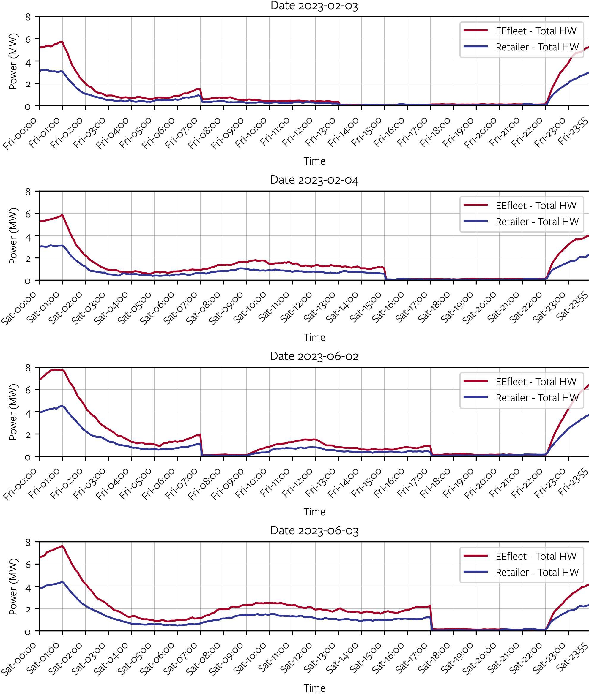
In this trial, EE operates their fleet of controlled loads based on the day of week and the month of year as described in Table 3 Figure 13 shows this operation strategy over 4 days chosen from two sample months with weekdays and weekends A specific retailer represents around 37% of customers which is denoted by ‘Retailer’ and the rest of the fleet is shown as ‘EEfleet’. As seen in Figure 13, the daily operations remain similar across different days for both the retailer and the rest of the fleet
Table 3 Control strategy of Endeavour Energy fleet of controlled load
Months Day type Nighttime period (AEST) Daytime period (AEST)
Figure 12. Number of customers with available market and PQ data at a 5-minute resolution throughout the year
Oct Weekday 22:00 – 08:00 09:00 – 18:00
Weekend 22:00 – 07:00 07:00 – 18:00
Apr – Sep Weekday 22:00 – 07:00 09:00 – 17:00
Weekend 22:00 – 07:00 07:00 – 17:00
Figure 13. EE fleet and retailer control strategy on different days of week and months (2023-02-03 and 2023-06-02 are weekdays and 2023-02-04 and 2023-06-03 are weekends)
From 8th of Sep 2023, the retailer started a dynamic scheduling strategy which varies across different days considering wholesale energy price and their prediction of consumers’ demand. Figure 14 illustrates the retailer’s dynamic strategy versus static schedule of the rest of fleet in four sample days between 6th-9th Oct
2023. Here, RRP is the regional reference price in NSW As seen, in most cases, the retailer has managed to shift their DEWH load to the periods when energy price was low. Further, it can be observed that there is significant volatility of price during daytime. An instance where price peak coincides with shifted DEWH demand can be observed on 2023-10-07 at around 13:00
Figure 14 Retailer's dynamic control strategy versus EE static schedule
Figure 15 shows the daily percentage of the shifted DEWH load into daytime period across 12-month period Minimum load shift occurs during Jan-Apr with the static scheduling. From the beginning of Apr till Oct, the implemented static load shifting scheduling shifts more load to the daytime and the percentage of shifted DEWH energy is greater on the weekends because the controlled load circuit is available for longer periods during the day It can be observed that the retailer’s dynamic strategy starting from Sep has significantly outperformed the static one in shifting DEWH load into the daytime period where the percentage of shifted DEWH energy can go higher than 70% on some days.
Figure 16 shows the total monthly DEWH energy that is shifted to daytime for each month per household As seen, shifted hot water energy is greater during winter months and the retailer also increases the shifted energy significantly towards the later months of the year with dynamic scheduling The total DEWH energy demand throughout the analysed 351 days is around 18,000 MWh and the total shifted load into the daytime is around 5,000 MWh, corresponding to an average shifted DEWH energy of about 28%. The average daily DEWH demand for a household is ~7kWh. During winter months there is an average 4.9 kWh of daily DEWH energy per customer that is shifted into the middle of the day for solar soaking
There are wholesale market financial benefits from shifting DEWH demand into daytime compared to the traditional controlled load where DEWH is heated during the nighttime. This is because abundance of rooftop
Figure 15 Daily percentage of the shifted DEWH energy into the daytime period
Figure 16. Total daytime hot water load per customer
solar and other utility renewable energy generation lowers the wholesale prices in the middle of the day. Figure 17 shows the estimated revenue from this price arbitrage per customer for each month. As seen, by shifting more load into daytime from Sep, the retailer has managed to significantly increase their revenue per household compared to the rest of the EE fleet. The average wholesale revenue is calculated to be ~$27 per customer for the studied 12-month period, noting that this revenue will increase with increasing rooftop solar and renewable energy generation in the network as well as retailer’s evolving strategy in shifting higher percentage of DEWH energy into daytime
Shifting DEWH demand to daytime also results in emissions reduction as during the daytime the grid has a higher percentage of renewable energy generation with lower CO2 emissions. Throughout the studied 12month period, it is estimated that around 1 kt-CO2 emissions were saved because of shifting DEWH demand into the daytime period Compared to traditional controlled load with nighttime heating, the trial resulted in 8% reduction in emissions associated to water heating.
4.3 Summary
The key points discovered through the real-world data analysis can be summarised follows.
• Throughout the 12-month analysed period, there has been 18,000 MWh of DEWH energy of which, around 28% has been shifted to daytime.
• With average 7kWh daily DEWH energy per household, there is significant potential in using the DEWH fleet for solar soaking purposes in NSW
• Dynamic orchestration by the Retailer towards the end of the analysed period significantly outperforms the EE static load control strategy in shifting DEWH energy into daytime, i.e. 74% vs 16% during the last days of 2023.
• The higher percentage of DEWH shift is promising however, it is important to ensure the household water amenity is not impacted. This should be checked and validated through customer surveys
• Despite volatility of wholesale energy price in daytime, the Retailer has been able to effectively shift the DEWH to price valleys With taking advantage of lower renewable energy prices during the day, there is considerable wholesale market financial benefits for retailers. According to analysed 12-month period, the average wholesale benefit is $27 per household but the daily benefit i ncreased significantly in the later months as the Retailer shifted a higher percentage to daytime.
Figure 17. Estimated revenue from price arbitrage per customer
• Currently households whose DEWH is controlled by smart meters can’t utilize their solar generation for water heating because the DEWH is installed on a physically separate electrical circuit than the solar. Moreover, the existing retailer tariffs don’t pass the potential wholesale arbitrage benefits on to households that can be achieved by controlling DEWH via smart meters ($27/year as highlighted above). It is recommended that retailers should design new tariff arrangements that will pass these benefits onto households including much lower import rates during solar generation period.
5 Impact of DEWH operation on the distribution network
5.1 Introduction
Due to voltage-to-power sensitivity of network at each household node, operation of a DEWH is accompanied with a local voltage drop. This phenomenon can be seen in Figure 18, where spikes in DEWH load is concurrent with a drop in voltage profile demonstrated for a sample household.
Voltage is mainly affected locally, but it is also influenced by other electrical dynamics within the network including loads and rooftop solar generation of other households that are on the same feeder An average voltage-drop corresponding to each ON-OFF operation of DEWH for each household is calculated and presented in Figure 19 Figure 19-a demonstrates the results for all qualified samples of ON-OFF operation of DEWH and the median voltage-drop for the whole fleet is 1.0V while the 95th percentile value is 4.8V.
Voltage-to-power sensitivity is a useful measure of network strength, where higher voltage-drop values with similar DEWH rated power indicate weaker connection points. In this analysis, 175 smart meters were identified as “critical” experiencing voltages above the upper threshold of 253V, which is maximum 10% allowed deviance from nominal voltage of 230V. Figure 19-b, shows distribution of voltage-drops for these meters, where it shows higher voltage-drop values with the median and 95th percentile values of 1.4V and 7.2V, respectively.
Since resistive loads vary with the square of voltage, voltage measurements are used to normalize the power consumption of DEWHs for a more accurate estimation of their rated power as illustrated by Figure 20 According to Figure 20, 3.6kW systems are the most common DEWH type for the studied fleet, followed by 4.8kW systems. Here, around 42 DEWH are identified as heat pumps with a rated power of 0.8 1kW.
Figure 18. Example of voltage-drop caused by DEWH load operation
Figure 19. Distribution of voltage-drop caused by DEWH operation
Figure 21 shows the distribution of voltage-drop for different DEWHs as grouped by their rated power Normally, operation of DEWHs with higher rated power causes higher voltage-drops. Nevertheless, this difference across DEWHs with different power ratings is negligible due to the low voltage-to-power sensitivity, indicating the strength of the EE network The unusual distribution observed for the 1.8kW and 2.4kW systems is due to limited number of the households with these DEWH types.
The low voltage-drops by DEWH operation implies the network strength and small power loss across the lowvoltage (LV) network This physical advantage might enable the DNSPs to incetivise consumers for provision of a voltage regulation service since operation of one DEWH customer could lower the voltage of other sites. This phenomenon can be evaluated by analyzing the correlation between voltage profiles of the households connected to the same LV network Figure 22 presents an example of daily operation of 6 out of 43 customers located on the same LV network. It is observed that voltage profiles are highly correlated and votlage of a site is impacted by the DEWH load on other sites
Figure 20. Classification of DEWHs rated power across Endeavour Energy network
Figure 21. Distribution of voltage-drop across different DEWHs types
Correlation of the voltage profiles of each pair of sites that are on the same LV transformer are also calculated for a sample day for more detailed analysis. Figure 22 shows distribution of these correlations for 14 LV transformers with at least 20 households located in Albion Park, NSW. According to Figure 23, except transformer 2 (T2) and transformer 5 (T5), the voltage profiles of customers on the rest of LV transformers are highly correlated.
The voltage correlation values could vary over time as impacted by the household behaviours and the network control schemes. Calculating an average correlation for each transformer on each day, the distribution of average daily correlations for each transformer is illustrated in Figure 24 across the year As seen, except T2 and T5, the correlation is fairly high across other LV transformers, indicating the potential for provision of voltage regulation services at all times, especially on T1, T6, and T8. It is noted that currently, voltage regulation service is not being traded in Australian distribution networks Nevertheless, the conducted analysis aims to inform the industry of possible viability of such initiatives.
Figure 22. Example of 6 DEWH operations and a highly correlated LV network
Figure 23. Correlation of voltage profiles on the same LV transformer
5.2 Operation of the whole fleet
DNSPs are interested in understanding how control strategies of retailers impact the network compared to their static controlled load operation schedule. Figure 25 shows the total DEWH load and the total net export (from the network perspective i.e. DEWH load plus general supply minus solar generation) presented along with the 99th, 95th, and 50th percentiles of voltage profiles which are calculated at each timestamp Results are shown for the Retailer and the rest of EE fleet on two sample days in Oct 2023. As illustrated by Figure 19-a, most of the trial customers experience small voltage-drops which indicates they belong to strong connection points. Thus, the 50th percentile voltage profiles are most likely corresponding to these customers. The 95th and 99th percentile voltage profiles, on the other hand represents customers that experience higher voltages. Thus, these customers (Figure 19-b) are most likely on weaker connection points
In a strong network, such as those connection points represented by the 50th percentile profiles, the voltage profiles are highly correlated and as a result, the voltages of groups of households would be affected by the DEWH loads operation of other households. The amount of such impact would depend on the amount of load being operated as well as the voltage-to-power sensitivity. Nevertheless, the difference between the retailer’s customers and the rest of the fleet would be minimal as observed in Figure 25. This minimal difference is because the retailers’ customers are randomly spread across the network and their voltage profiles are highly correlated with the neighbouring customers belonging to the rest of the fleet.
On the other hand, Figure 25 also shows that the implemented control strategy has minimal impact on the 95th and 99th percentile voltage profiles since the retailer’s profiles closely follow those of the rest of the fleet These profiles corresponding to the households with higher voltages located in weaker parts of the network have smaller voltage correlations with the rest of the fleet. For these customers only the local consumption of power can impact their voltage rather than the operation of the fleet.
With the current level of network load, solar penetration, and for most of the customers, this outcome might enable EE to further accommodate retailers with freedom of deploying market-driven control strategies without having major concerns about network bottlenecks. Nevertheless, it also demonstrates the limitations of random grouping of customers. In other words, to help with voltage regulation of those customers in the weaker parts of network, it is suggested that more advanced location-based control strategies should be used.
Figure 24 Distribution of daily correlations for different LV transformers in Jan-Dec 2023
Also observed in Figure 25, the voltage profiles are higher at nighttime than daytime which is counter intuitive since daytime solar generation generally leads to voltage rise. This issue can be understood by the EE voltage control scheme in daytime period, lowering zone substation voltage reference to maintain safe limits and avoid PV curtailment. While such strategy may be effective, in the long run, it can impact the lifespan of power equipment due to frequent switching incurring costs on the system. Being a highly predictable load, as discussed in the next section, DEWHs could assist with voltage regulation if orchestrated intelligently with the aim of minimising power imbalance This can provide a smoother voltage profile as well as reduce the need for active voltage control mechanisms.
5.3 Analysis using network modelling
This section presents the analysis conducted on the Albion Park network model using DIgSILENT PowerFactory 19 , a specialized software used for power system analysis and electrical engineering applications. This section is aimed to show voltage response of the network according to different DEWH control and orchestration strategies
Figure 26 shows the total DEWH load corresponding to 31 customers along with 99th and 95th percentile values of voltage among all 109 nodes for different operating scenarios at a LV transformer. CL1 corresponds to the case where all DEWH heating takes place at nighttime and CL3_25, CL3_50 and CL3_75 corresponds to the three different control strategies where 25%, 50% and 75% of daily DEWH energy are shifted to solar generation window, respectively As seen, the scenarios with higher DEWH load tend to result in lower voltage profiles at any given time, which can help with voltage regulation during daytime where solar generation can lead to voltage rise.
19 DIgSILENT PowerFactory, available here
Figure 25. Operation of the whole fleet on two sample days in 7th-8th Oct. 2023
Figure 27 presents the difference between power and voltage metrics of the three CL3 control strategies with different percentage of shifted DEWH load against the traditional CL1 control strategy. As seen, the drop of voltages during daytime increases with higher percentage of DEWH load that is shifted into daytime and the voltage drop is greater for 95th percentile value than the 99th value
Figure 26. Two sample days operation of DEWH load under different control strategies for a LV transformer
Heat pumps are gaining popularity in Australia supported by different government rebates due to their higher energy efficiency Heat pumps have smaller rated power and energy consumption as per their COP which could limit their impact for voltage regulation. Nevertheless, compared to resistive DEWH, they run for longer periods of time for the same electric energy demand, which could lead to a long-lasting impact on the voltage profiles. Thus, simulation of scenarios with high penetration of heat pumps is of interest. Moreover, with the ongoing electrification efforts, it is expected that penetration of DEWH increases significantly, which means there is increasing opportunities for DEWH load for network support in the future. Therefore, future cases where all households own a DEWH is also studied as part of the simulations
Figure 28 demonstrates the difference of 99th percentile voltage profiles between CL1 and the other three CL3 profiles in four case studies. Case A represents the actual data for households where 31 out of 109 households are DEWH customers with actual rated power values. Case B represents if 31 out of 109 household owned a heat-pump rather than the actual DEWH types The hypothetical cases where all households own a DEWH is denoted with “DEWH100” when the households owned resistive DEWHs (Case C) and “DEWH100_HP” when they owned a heat-pump (Case D). The comparison of Cases A and B with Cases C and D reveals that as DEWH penetration rises, the magnitude of the voltage impact increases considerably.
Cases B and D show that as heat pumps become a major DEWH type, the potential voltage impact for network support may decrease Finally, the simulations reveal that there can be smarter orchestration of DEWH with more effective randomisation and location-based strategies to schedule the DEWH load over a longer time span
Figure 27. Impact of shifting DEWH load into daytime on voltage metrics compared with CL1 scenario
during the day to obtain a smoother voltage profile Otherwise, the voltage drop profiles exhibit local peaks as shown in Figure 28.
5.4 Summary
• Analysis of the real-world power quality data shows small voltage-to-power sensitivity, indicating a high network strength for most of the DEWH customers
• It is found out that customers on several LV networks possess highly correlated voltage profiles, indicating potential for utilizing flexible demand as a voltage regulation service.
• Analysis of the voltage statistical metrics reveals that for those customers experiencing higher voltages, the operation strategy of the fleet is ineffective. This implies the need for more intelligent location-based controlled load strategies to impact such customers.
• Network modelling using PowerFactory software indicates that with uptake of heat pump technology, the potential of DEWH load for voltage regulation may significantly decreases.
• PowerFactory simulations show that networks with higher penetration of DEWH customers observe larger voltage drop from shifting load into daytime window. Nevertheless, traditional static control schemes are not effective in maintaining a smooth aggregated power. Thus, intelligent location-based methods are necessary.
Figure 28. Impact of shifting DEWH load into daytime on the 99th percentile voltage under four case studies
6 Forecasting aggregate DEWH demand on the network
6.1 Introduction
This section presents research findings on forecasting day-ahead DEWH energy, which could be useful to network operators as well as retailers. The analysis shows that total daily DEWH demand is closely correlated with average ambient temperature as well as the operating control strategy. Figure 29 illustrates this relationship, showing that lower temperatures typically align with peaks in hot water demand, while warmer days see reduced demand. In addition, it is observed that regardless of temperature there are demand spikes on weekends, where DEWHs experience longer heating windows. Moreover, a lag is observed between DEWH load and temperature changes, which can be attributed to the thermal inertia of DEWH storage tanks. In addition, household behaviours in different times of year also impacts DEWH demand.
6.2
Method and results
Using various machine learning algorithms, a method developed by UNSW team based on one-year available data demonstrates significant potential for accurately predicting DEWH demand. This report presents the results obtained by applying a hybrid model combining convolutional neural networks (CNN) and long shortterm memory (LSTM) networks at two levels of aggregation: the entire DEWH fleet and the zone substation. This model employs advanced deep learning techniques, using CNNs to identify correlations between DEWH demand and ambient temperature and LSTMs to capture demand patterns over successive days. The developed model uses data from five consecutive days, including total DEWH demand, average dry-bulb temperature, and day of week along with the forecasted average temperature for the next day as inputs, to predict the total DEWH demand for the following day. For training and testing this forecast model, the data was divided into alternating fortnights, with half serving as the training set and the other half as the test set.
For the aggregated DEWH load of the entire fleet, Figure 30 displays a normalized scatter plot where the vertical and horizontal axes represent the model’s predictions and the actual measurements, respectively. The model’s high accuracy is evident from the close alignment of data points along the ideal black diagonal line. To quantify this performance, the coefficient of determination (R²) and mean absolute percentage error (MAPE) were calculated, yielding R² = 0.956 and MAPE = 4.1%. This high R² and low MAPE indicate strong model accuracy. Figure 31 further illustrates the predicted and actual DEWH demand which are plotted for the test set over the year.
Figure 29. Daily total DEWH demand versus mean temperature
31. Actual versus predicted DEWH demand on an alternating fortnightly split dataset
At the zone substation level, 13 out of 155 substations, serving at least 117 customers, were selected for testing the DEWH load forecasting model. Figure 32 displays the R² score and MAPE for each of these substations. As shown, the R² score exceeds 0.89, and MAPE is below 7% in all cases, highlighting the model’s high accuracy and the predictability at the substation level. It should be noted that the reported performance here can be further improved via additional model hyper-parameter tuning which will be investigated if the forecast models are found to be useful by DNSP or retailer partners
Figure 30. Scatter plot for a predictive model comparing estimated and actual next day DEWH demand
Figure
Figure 32. Performance of the DEWH load forecast model at substation level aggregation
6.3 Summary
• The aggregated daily DEWH demand in EE network is highly correlated with ambient temperature as well as the controlled load scheduling scheme.
• Applying machine learning methodologies on available data, the day-ahead DEWH energy can be predicted with high accuracy as R2 score over 0.95.
• Preliminary study on the zone substation level with over 117 customers shows significant performance with a MAPE of less than 7% in several LV networks.
7 Discussions and conclusions
7.1 Discussions
SolarShift projected has investigated the water heating technology options for Australian households from various angles including thermal modelling, customer hot water roadmap, network impact and modelling and forecasting of day ahead hot water demand. The key insights and their implications are discussed in this section as below:
7.1.1 Thermal modelling
• Thermal modelling results show that average storage efficiency for DEWH tanks range between 6772%. This significant loss of energy from DEWH tanks could be reduced by improving the quality of tank and pipe insulation, which can bring significant financial and emissions savings for households.
• The report presented preliminary insights on the energy and cost savings with better insulation, a more detailed cost-benefit analysis can be carried out in collaboration with DEWH manufacturers. The outputs can also inform relevant Australian Standards which can be incorporated in minimum energy efficiency requirements for DEWH storage tanks.
• The type of DEWH control strategy has a bigger impact on the thermal efficiency than the hot water draw profile (HWDP) which is a result of household behaviour. This indicates that external control strategies have great importance in improving energy efficiency of DEWH.
• More predictable HWDPs result in more predictable DEWH tank behaviour which provides higher flexibility for DEWH control.
• The main factors that determine the emissions associated with water heating are grid energy mix, DEWH technology (i.e. resistive, heat-pump, gas, etc), and heating period, where heating shifted to solar generation windows results in lowest emissions. Heat-pumps result in an average of 67% lower emissions than R-DEWH
7.1.2 SolarShift Customer Hot Water Roadmap
• The developed method provides a clear breakdown of the finances associated with water heating. To further assist Australians with understanding of their hot water system and tariff options, the method will be developed into an online Customer Hot Water Roadmap Tool where households can get bespoke results and suggestions for their unique cases
• The analysis clearly shows that there are various important variables impacting the finances of water heating apart from the technology. These include control strategy, tariffs, ownership of rooftop PV as well as capital and other costs.
• Results show that households with rooftop PV, a heat pump and timer set to solar soak hours returns the lowest annual water heating bill.
• Net present costs (NPC) highlight there may be financial barriers for households buying a new higher cost heat pump and solar thermal heaters due to their high capital cost. Lower cost heat-pumps return a lower NPC, however their longevity as predicted by their warranty period are key factors that also needs to be considered
7.1.3 Real - world analysis of Endeavour Energy Off peak plus trial data
• This research has discovered that most DNSPs, outside of Victoria and Queensland, are likely to give the control of smart meters and DEWH to retailers The Solarshift project team made many attempts to engage a retailer partner within this project but were not successful. As a result, UNSW and EE were not able to directly control DEWH fleet within the trial.
• Despite this challenge, UNSW team has produced valuable research outputs via analysing real-world trial data and undertaking network modelling It was shown that on average 28 % of daily DEWH energy was shifted to solar generation period. This percentage significantly increased to 60-74% towards the end of the trial as the retailer gained more confidence in control and orchestration.
• Our analysis found that there was on average $27 per customer financial savings opportunity over the studied 12-month period through wholesale arbitrage which are anticipated to grow as there are more DEWH load and renewable energy generation in the network. However, these benefits are currently not passed onto the households as most of the existing tariffs don’t have access to wholesale prices and they don’t include a cheaper daytime component.
• This raises an important point for the future of DEWH flexible demand since the percentage of DEWH fleet on controlled load has rapidly decreased over recent years. 20 There needs to be appropriate incentives for households to install their DEWH on a controlled load and thereby allowing control of their DEWH to retailers/aggregators via smart meters for orchestration
• Throughout the 12-month study period, it is estimated that around 1 kt-CO2 emissions were saved because of shifting DEWH demand into the daytime period for the analysed ~7,300 DEWH. Compared to traditional controlled load with nighttime heating, the trial resulted in 8% reduction in emissions associated to water heating.
7.1.4 Impact of DEWH operations on networks
• Operation of DEWH results in a voltage drop at the household connection point, and the size of the voltage drop depends on other network and electrical variables apart from the DEWH load itself.
• The median voltage drop associated with DEWH operations is calculated as 1V however this voltage drop is greater at 1.4V for critical meters which experience voltages above 253V. This voltage reduction can help to improve power quality and reduce potential rooftop solar curtailment for these critical sites.
• Voltage correlation across the households were high within the EE network which indicate strong network and flexible demand of DEWH can be utilized to regulate voltages on other households.
• The studied network modelling has shown that daytime voltage drops increases with higher percentage of shifted DEWH demand into the day. The potential voltage impact is greater for RDEWH than heat-pumps due their higher current draw. Smart scheduling and orchestration of DEWH are important for obtaining smoother and prolonged voltage drop profiles.
7.1.5 Forecasting aggregate DEWH demand on the network
• Daily DEWH demand is highly correlated with ambient temperature
• The developed deep-learning forecasts models can predict day-ahead aggregate DEWH demand in the network accurately through using ambient temperature and historical DEWH demand as main inputs
• The forecasts are successful both at both entire fleet and substation levels.
• These accurate day-ahead forecasts can assist with day-ahead operations of DNSPs and retailers especially when planning for flexible demand operations and rooftop solar/CER management.
20 Electric water heaters is a hero of flexible demand. Where does it stand in the age of rooftop solar?, available here
7.2 Next steps
Flexible DEWH demand is an important asset for households, networks and retailers. We need to ensure that this asset is utilized in a smart and equitable way to help transition towards the Australian’s low carbon energy future. There are various future research directions that the research team has identified to continue progressing the work. These are summarized below:
• DEWH storage tanks have high energy losses up to 1/3rd of total energy input. These losses can be minimized via improved insulation of the tanks and pipes. A cost & benefit and DEWH thermal performance analysis can be undertaken in collaboration with DEWH manufacturers to investigate this area in more detail. This can potentially inform regulatory, and standards process on the minimum energy efficiency and insulation requirements for DEWH storage tanks.
• UNSW team can work on developing smarter DEWH control algorithms to control and orchestrate DEWH fleet with a retailer partner who has control over the smart meters. Leveraging the outputs from thermal and network modelling will help in developing highly energy and cost-efficient control algorithms to benefit households, networks and retailers.
• Heat pumps have become a popular DEWH heating technology because of their higher energy efficiency and support by the government incentives and rebates. These units have smaller rated power though require longer operational periods, and some heat-pump manufacturers don’t recommend external control of these units due to unpredictable interruption of the compressor unit and potential reduction to its service life Control and orchestration algorithms may need to be further refined for heat-pumps compared to resistive units.
• The research on the customer hot water roadmap will continue and UNSW team will build a public facing online tool to utilize the research outputs. This tool will allow customers around Australia to match their specific living conditions, including their location, household size, hot water usage patterns and current water heating system, to generate customised insights on the financial and environmental aspects of different water heating systems The tool is aimed to empower customers when making a choice on water heating systems and technologies.
• Power flow models built for analysing the network impact of DEWH have given useful insights. Future simulations will include the analysis of different rooftop solar and DEWH penetration to give further insights on possible future scenarios and DEWH’s potential role and impact on voltage management.
• Developed DEWH load forecasting models have given highly accurate results. It would be interesting to apply these models in real-world DNSP and retailer operations to gain further insights on potential use cases and associated benefits with improved management of flexible demand and CER.
• Thanks to smart meters and the quality of interval data they produce, advanced data -driven modelfree power flow methods can be developed and integrated into the DEWH load operation strategies to more effectively assist with network voltage regulation
Appendix A: Nomenclature and abbreviations
Table 4. Nomenclature
Abbreviations
Explanation
DSC Daily supply charge Costs
SFIT
Solar feed - in tariff – missed opportunity costs from using solar generation rather than exporting to the grid
CL Controlled Load
tou Time of Use
GS General Supply
SS Solar Soak
OP Off - Peak
HWDP Hot Water Draw Profile
DEWH
R - DEWH
HP - DEWH
Domestic electric water heating system
Resistive type domestic electric water heating system
Heat - pump type domestic electric water heating system (used interchangeably with heat - pump, HP)
HP Heat - pump (used interchangeably with HP - DEWH)
DNSP Distributed network service provider
Plot Legend
R - DEWH - nPV
R - DEWH - PV
HPhc - nPV
HPhc - PV
HPlc - nPV
HPlc - PV
Resistive domestic electric water heater with no PV
Resistive domestic electric water heater with PV
Higher cost heat - pump with no PV
Higher cost heat - pump with PV
Lower cost heat - pump with no PV
Lower cost heat - pump with PV
STC Electric boosted solar thermal water heater
GI Gas instantaneous water heat
GStg Gas storage water heater
IC Initial Costs
US Usage Costs
MC Maintenance Costs
DSC Daily supply charge Costs
SFIT
Solar feed - in tariff – missed opportunity costs from using solar generation rather than exporting to the grid
Appendix B: Parameter Descriptions and Assumptions
Solar thermal heater (315L), Rheem, Split system, supply and install
Gas storage heater (170L), Rheem, NSW supply and install 1785
Gas instantaneous heater (26L), Rheem, supply and install 1322
Resistive maintenance
Heat pump maintenance
Solar thermal maintenance
Gas storage maintenance
Gas
Establish
Including
technology certificate rebate
• Every 4 years
• Anode replacement
• General maintenance
• Every 4 years
• Anode replacement
• General maintenance
• Every 4 years
• Anode replacement
• General maintenance
• Every 4 years
• Anode replacement
• General maintenance
Table 6. Ausgrid DNSP tariff rates, taken as an average on Origin, AGL and Energy Australia Rates
Tariff Name
Ausgrid CL 1
Ausgrid CL 2
Ausgrid CL 3
Ausgrid flat
Ausgrid tou
Tariff Rate ($AUD)
DSC = 0.00/day
Rate = 0.179/kWh
DSC = 0.00/day
Rate = 0.179/kWh
DSC = 0.00/day
Rate = 0.179/kWh
DSC = 1.01/day
Rate = 0.370/kWh
SFIT = 0.0500/kWh exported
DSC = 1.12/day
Peak rate = 0.645/kWh
Off-peak rate = 0.251/kWh
Shoulder rate = 0.346/kWh
SFIT = 0.0500/kWh exported Gas DSC = 1.0549/day
0 – 20.71MJ = 0.0545/MJ
20.71 – 41.1MJ = 0.0386/MJ
Table 7. Customer hot water roadmap general assumptions
General Assumptions
• PV system used for analysis: 5 kW AC rooftop PV system
• Households with solar thermal water heaters will not also have a PV system
• Solar thermal heater will only be considered for households with 3 or more people
• Lower cost heat pump will only be considered for households of 4
• Controlled load (CL) strategies are modelled with self - consumption assumption for cases with PV (i.e., as if they can switch circuits between the general supply & controlled load). In reality this is not possible as hot water system are connected to a separate electrical circuit. This assumption allows a potential future scenario where switching between the control load and general supply is possible
• State specific supply and installation costs are considered where possible, and an average is taken where it is not.
• Solar feed in tariff (SFIT) is considered as a missed opportunity cost when it is used for water heating The s olar generated power is self - consumed rather than exported/sold to the grid at the rate specified by energy retailers
• Daily supply charge for electric systems connected to general supply not included in cost calculations (because household will have electricity for all other loads from general supply)
• Additional DSC specially for CL tariff is taken to be zero, as outlined by energy retailers in 2024 - 25 energy prices. It should be noted that DNSPs do include an additional DSC for controlled load circuits that is seemingly not passed on by energy retailers . Additionally, DNSP rates reveal different pricing for CL1 and CL2, energy retailers price the two CL rates the same.
• Gas daily supply charge (DSC) included in analysis, assumed when switching to an electric system gas account is not closed and the DSC will continue to be billed
• Weather data: Meteonorm’s TMY files for main cities in Australia (included in TRNSYS)
• For all systems with hot water storage tanks
o Thermostat high temp = 65ºC
o Deadband = 10ºC
o Hot water consumption temperature = 45ºC
• Average daily hot water draw for household with 4 people = 200[L/day]
• PV option represent best case scenario, real results fall somewhere in - between this best - case scenario and nPV (no PV) options
o In best case scenario, it is assumed water heating has priority over household load
Table 8. Customer hot water roadmap technology assumptions
Technology Assumptions
Heat Pump:
• Heat pumps considered are Reclaim Energy, glass lined heat pumps with a warranty of 10 years – more upper market option
o Variation for household size
• Lower cost heat pump considered is the iStore heat pump with a warranty of 5 years and a lifespan of a similar time
Gas:
• Modelled with 80% boiler efficiency, calculated based on technical data
• Methane for heat value (47 MJ/kg)
• Rheem gas storage and gas instantaneous heaters considered
o Variation for household size
Electric Resistive:
• Rheem electric resistive heaters considered
o Variation for household size
• All tanks have same values for losses (0.9W/m2 - K) – not included in technical data
• Efficiency of 1
Solar Thermal:
• 4 square meter system
• Using standard values for optics and thermal losses
o FRta= 0.6
o FRUL = 0.6 W/m2 - K
o IAM coefficient = 0.2
• Electric auxiliary heater
• Rheem loline solar thermal heater considered
Table 9. Net present cost assumptions
Net Present Cost Assumptions
Determined based on implementing an entirely new system, potential rebates for switching or upgrading old water heaters not included, however Small - scale Technology Certificate rebates are included.
Considering net present costs over a 10 - year period with a discount rate of 8%
Scenario of reinvestment in cheaper heat pump is considered where system is replaced within the 10 - year period (a second new system within bought in the 10 - year period)
Table 10. Payback period assumptions
Payback Period Assumptions
Initial cost for current/old heater
• Switching from resistive – initial costs included
• Switching from gas storage – initial costs = $0
If payback period > 20 years, plotted as 20 years
If payback period < - 20 years, plotted as - 20 years
Switching cases considered switching between same tariff/control type
• E.g. switching from a resistive heater on CL1 to a heat pump on CL1
Inclusive of state specific rebates for upgrading and switching scenarios (rebates for heat - pumps and solar thermal and in some cases resistive if you are switching from gas)
Appendix C: tm_solarshift open-source repository
The thermal simulations are carried out using the open-source repository “tm_solarshift” built specifically for this project. It is an object-oriented codebase providing a set of modules to perform thermal simulations, define control strategies, manage weather data and other timeseries profiles, specifically for domestic water heating systems. The python repository architecture is presented in Figure 33 .
Figure 33. Architecture of the Python codebase for DEWH management system. The package uses TRNSYS as the numerical engine to simulate the DEWH systems. TRNSYS is a commercial simulation software, widely used in renewable energy and building engineering, designed to perform fast annual simulations of complex interconnected systems. It includes an extensive library of component models (called Types) as well as tools for control and analysis. In the case of hot water systems, it includes 1D models for tanks that take into account the thermal stratification on the tank. TRNSYS is a widely used and accepted thermal simulation tool however, the main drawback is that testing different configurations and input parameters can be challenging because automating these simulations is not straightforward. Additionally, integrating external code from other sources like Python is not simple, and it does not allow external libraries (such as numpy, pandas, or scipy). For these reasons, this repository is almost completely based on Python, using TRNSYS only as the DEWH tank thermal engine.
A simulation is defined in this repository by four steps:
a) Defining the simulation settings (blue box in Figure 33),
b) Generating the timeseries required for the simulations (purple box),
c) Running the thermal simulation on TRNSYS with the conditions defined in the previous steps (orange box), and
d) Post-processing and analysis (grey box).
In the first step (simulation settings), three types of objects are created: General objects, Timeseries Generators and Models. The General objects contain the “real-world” data, such as the household’s location, energy plan, and device’s technical specifications. The Generators are modules designed to provide the required time- series using external sources (such as market or weather data) and/or synthetic data methods (for HWDP or control randomization). For DEWH system, specifically, TRNSYS models required weather variables (ambient and mains temperatures), hot water draw profiles (HWDP), and tank control signals. The Model objects run the simulations using the data provided in the previous two steps. In the results presented in this report, the most important object is the DEWH Model, which includes methods to run the TRNSYS simulations.
TRNSYS simulations are set using its graphical user interface (GUI) layout tool called Simulation Studio. Three layouts were developed in this research, one for immersive resistive heaters, one for heat pumps, and one for solar thermal collectors. Figure 34 shows the layout for resistive heaters. On the resistive layout the following types (which corresponds to components in TRNSYS nomenclature) were used:
• Type 158: cylindrical storage tank with multiple ports and auxiliary heaters.
• Type 1226: Electric water heater with control signal.
• Types 647 and 649: mixer and flow diverters, respectively,
• Type 9a; plain-text data reader, used for timeseries,
• Type 953: controller for tempering valve,
• Type 1503: N-stages Aquastat, as maximum temperature control,
• Type 25c: printer for outputs (as plain text).
• Type 42b: double interpolator (for heat pump), and
• Equation types.
Figure 34. Layout in TRNSYS for resistive heater.
Appendix D: Additional results for thermal simulations
In this section, the results for storage efficiency and annual electricity consumption are presented for Adelaide, Brisbane, and Melbourne
35. Storage efficiency (left) and annual energy consumed (right) for different HWDP and control loads in Adelaide.
36. Storage efficiency (left) and annual energy consumed (right) for different HWDP and control loads in Brisbane.
• The provided network by EE includes ~11,000 households and ~600 of them is matched with the actual household location based on their LV transformer.
• For these households, both the general supply and controlled load circuits are modelled.
• For all loads except households with DEWH, a year of hourly average power consumption profile is utilised.
• PV systems are simulated with a 24-hour half-hourly average profile.
• The general supply circuit of DEWH customers is simulated with the real-world 5-minute market data.
• Total daily DEWH demand for each customer is calculated based on the real-world data.
• The rated power of each customer is set based on the classification presented in Figure 19
• Scenarios of operating and shifting DEWH load into daytime is simulated as follows.
o CL1: All daily DEWH demand is allocated during nighttime period, i.e. 10:00 pm – 07:00 am.
o CL3_x: x% of the DEWH load is shifted to the daytime period, i.e. 09:00 am – 05:00 pm
• After determining the allocated kWh of energy for each customer in each heating window, the required heating time is calculated as a rounded number of 5-minute time slots. Nevertheless, the rounding error on the whole fleet is negligible.
• The DEWH load of each customer turns on based on a random number to assimilate the realworld randomisation of DEWH loads.
Figure 37. Storage efficiency (left) and annual energy consumed (right) for different HWDP and control loads in Melbourne.