Appendix E: Technical Notes and Limitations for the American Community Survey and Other Data Sources

APPENDIX E

Technical Notes and Limitations for the American Community Survey and Other Data Sources

POVERTY

There are many ways to analyze income and poverty for public health. Poverty is better to look at than household income in at least one respect—it adjusts for the size of the household. A household income of $100,000 is much different for a household of two people versus a household of eight. The poverty line is based on household size as well as income. The poverty rate is reported by individuals or by families, although poverty status is attributed from the household. The household poverty status is based on total household income and the number of people in the household according to the poverty guidelines from the U.S. Department of Health and Human Services. The poverty line is adjusted for Alaska and Hawaii, but for no other geographies. Thus cost of living is not reflected in calculating poverty. The poverty line, though, is considered much too low to sustain even a very meager lifestyle. Thus many government programs’ eligibility is determined by some multiple of poverty income. For this reason, the American Community Survey, in indicator C17002, reports on persons with ratios ranging from 50% of poverty level to 200%. Other tables (e.g., B17001) report the poverty level to 500% and over. The American Community Survey, combined with the decennial Census from 2000 and previous, allows trend analysis of poverty rates. For Census 2000 data, the Census Bureau’s American Factfinder may be used. For decennial Census data before 2000, the easiest site to use is the National Historical Geographic Information System at http://www.nhgis.org. This site gives both data from the decennial Census back to 1790 as well as ArcGIS-compatible boundary files. To download the poverty data from the American Community Survey, use the methods outlined in Appendix B and look for indicator C17002. This is the data on individual poverty for all races/ ethnicities combined. You can also download data for individual races/ethnicities; these are in the data following B17001, and include B17001A for Whites and B17001B for African Americans/ Blacks.

MEDIAN HOUSEHOLD INCOME

Median household income, indicator B19013 in the American Community Survey, is the standard method of measuring income. Another way to measure income, and a good way to compare between areas, is to calculate the percentage of households in the top income brackets versus the percentage in the lowest income brackets. For the American Community Survey, indicator B19001 may be used. The lowest bracket is less than $10,000 and the highest bracket is $200,000 or more.

GEOGRAPHIES WITH SMALL NUMBERS

Census tracts may have unreliable or unstable estimates because they are truly sparsely populated or have too few people per year living below poverty or other ACS indicators. Areas with few inhabitants typically include rural areas, restricted areas (e.g., airports, reservoirs, military bases), public open spaces (e.g., parks) or unincorporated areas. However, because in some Census tracts the non-response rate to surveys like the ACS might be higher than average due to population characteristics such as immigration status or race/ethnicity, a health department must determine through local assessment efforts if there are populations in their jurisdiction whom the ACS does not represent.

STATISTICAL RELIABILITY AND STANDARD ERRORS

Statistical reliability is one of the most difficult subjects to explain to people unfamiliar with data; however, it is one of the most important. When possible, this guide explains how to calculate standard errors and relative standards errors for indicators to assess data reliability. Assessing the data reliability through the relative standard error (RSE) is important to prevent misinterpretation of data, which could lead to inappropriate policies and poor resource allocation decisions. Generally, BARHII recommends the following for any indicator with a RSE greater than 30%: clearly indicate the estimate as unreliable on any map, table, or narrative with the following language: “these data are statistically unreliable, interpret with caution”; avoid using those estimates in any epidemiologic, or financial modeling, consider local data collection in those areas or use a different indicator. Statistical reliability of estimates could be improved by aggregating estimates to a higher geographical level, aggregating over time, or by collapsing categories.

APPROXIMATE STANDARD ERRORS FOR ACS DATA

The ACS uses a replicate-based methodology to calculate the standard errors of the sample weighted estimates it publishes. To create categories that go beyond those published by the ACS, standard errors for sums, differences, ratios, proportion, or products are derived using an approximate method that is documented in Accuracy of the Data, available at http://www.census.gov/acs/www/ data_documentation/documentation_main/. The standard errors obtained by the approximate method could either underestimate or overestimate the true standard error. Further, as the number of estimates involved in a sum or a difference increases, the approximate standard error will become increasingly different from the standard errors derived using the replicate method. Although

the accuracy of the standard errors could be improved by using PUMS data. These data are not available for smaller geographical areas such as Census tracts for confidentiality.

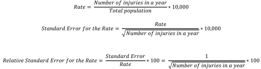
POISSON AND BINOMIAL STANDARD ERRORS

When working with data different to the ACS, standard errors might not be available. It is possible to approximate the standard error for Poisson (counts) and binomial variables (proportions) as follows: Poisson standard error (counts) example: annual injury rate per 10,000 people

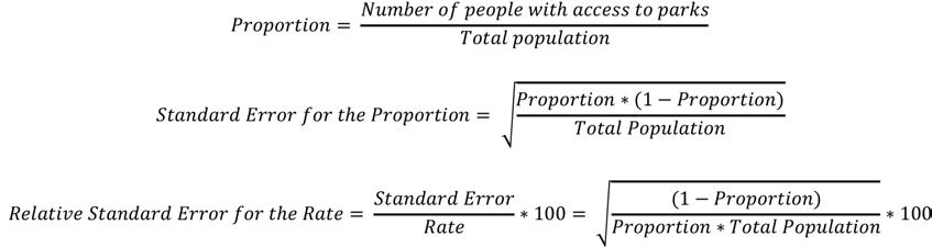
Binomial standard error (proportion) example: access to parks versus no access to parks

CONFIDENCE INTERVALS

In this guide, BARHII recommends calculating 90% confidence intervals for American Community Survey data because those are based on margins or error published by the Census. While a 95% confidence interval is a standard most often used in statistics and epidemiology, BARHII recommends to consider an 80% confidence interval for many of the social and economic indicators presented if less statistical precision is needed for a program or policy objective.

COLLINEARITY AND CONFOUNDING FACTORS: EFFECTS IN THE INTERPRETATION OF INDICATORS

Although they are important concepts in the literature about the SDOHs, this guide does not discuss collinearity or confounding, For example, a collinear relationship between poverty and educational attainment exist, potentially confounding the analysis between one of these determinants and health outcomes. Nevertheless, we believe that this limitation does not discredit the recommendations in this guide for these reasons: 1) The expertise required to properly account for collinearity in the SDOHs may be beyond the expertise of most LHDs, and is, therefore, a topic best reserved for research institutions. 2) One such landmark research project, the Harvard Health Disparities Geocoding Project, analyzed many SDOHs in various combinations, morbidity, and mortality and found that poverty alone consistently identified social gradients in health (citation below). This research supports this guide’s recommendations, especially recommendation 3 in the introductions, which recommends using poverty to identify places with the greatest health inequity, although collinearity between poverty and other SDOHs may exist.

AGGREGATES OVER TIME AND TIME DISCONTINUITIES

The advantage of aggregating data over time is an improved reliability of the estimates. The ACS combines population or household data from multiple years to produce statistically reliable numbers for small counties, neighborhoods, and other local areas. In general for any given area, the larger the sample and the more months included in the data, the greater the confidence in the estimate. The ACS collects data continuously and then aggregates the results over a specific time period to produce one-, three-, and five-year annualized estimates of population or household. In contrast, the decennial Census typically collected data between March and August. As a consequence, estimates might not be comparable between the ACS and the decennial Census. One advantage of spreading data collection evenly across the entire period is that it avoids over-representing any particular month or year within the period.

The key trade-off to be made in deciding whether to use single-year or multiyear estimates is between currency and precision. Multiyear estimates should, in general, be used when singleyear estimates have large RSEs or when the precision of the estimates is more important than the currency of the data. Multiyear estimates should also be used when analyzing data for smaller geographies and smaller populations in larger geographies. Multiyear estimates are also of value when examining change over nonoverlapping time periods and for smoothing data trends over time.

U.S. Census Bureau, 2008

Differences in data collection may cause time discontinuities: changes in a survey question or changes in the sampling universe (e.g., including or excluding group quarters).

CENSUS TRACT BOUNDARY CHANGES

Census tract boundaries can change each decennial Census. Census tracts with a significant change in population and in boundaries should be accounted for in any trend analysis. The Census publishes geographic relationship files that show the comparability for the same type of geography over different periods of time (e.g., the relationship between places in 2010 and places in 2000), including estimates on how the Census 2010 population is distributed within the boundaries of Census 2000 geographies. This information is available at http://www.census.gov/geo/mapsdata/data/relationship.html.

ACS DATA CENSORING

Because of privacy concerns, the Census tract is the smallest level of geography available for all social and economic indicators in the American Community Survey. The ACS publishes one-year estimates for areas with at least 65,000 people, three-year estimates are available for all areas with at least 20,000 people, and five-year estimates are available for all geographic areas down to the block group level.

RACIAL AND ETHNIC CLASSIFICATION BIAS

Understanding the SDOHs at a race or ethnic level is also challenging because the data often fail to account for different ethnicities within a race. Most SDOH indicators in their current form use broad race/ethnic categories (Asian, African American/Black, White, Other/Unknown, Multirace). These categorizations can be misleading. For example, an indicator will often describe the number of Asian people, but it fails to break out by Asian ethnicity (e.g., Korean, Chinese, Vietnamese). Furthermore, Pacific Islanders are often grouped together with Asians. Similarly, the category Hispanic/Latino does not account for the different countries of origin or cultures (e.g., Mexico, Argentina, Spain), and the category American Indian/Alaskan Native includes hundreds of tribes. These categories make it difficult to capture accurate race/ethnicity data, as people who complete the information may be identified incorrectly by someone else, or may not identify with the limited categories. In addition, these groupings make it difficult to develop population-specific health interventions because one ethnicity may have different cultural beliefs and practices about health behaviors (e.g., tobacco, diet) than another, although they share the same racial category. While some ethnicity-specific data are available at the Census tract, block group, and block levels, stratification by social or economic factors is limited. This is a significant limitation of SDOH indicators that can only be currently remedied by place-based population assessment and advocacy for more precise collection and reporting about race and ethnicity in SDOH datasets.

NON-RESPONSE RATE AND IMPUTATION

The U.S. Census Bureau estimates that the ACS non-response rate is about 10% for the overall population, but it might rise to 15 to 20% among undocumented migrants. One study indicated

that ACS non-respondents are different from respondents, and are more likely to be male, African American/Black, and between 25 and 44 years. To increase the accuracy of the population counts, the U.S. Census Bureau imputes the existence and number of people living at address with no response. The imputation methods either use rules to determine acceptable answers or use answers from similar housing units or people who provided the item information.

GROUP QUARTERS FACILITIES

A group quarters (GQ) facility is a facility owned or managed by an entity or organization to provide housing and possibly services for the residents, whom are usually unrelated people. GQs include college residence halls, residential treatment centers, skilled nursing facilities, group homes, military barracks, correctional facilities, workers’ dormitories, and facilities for people experiencing homelessness. Young adults and the elderly are more likely than other groups to be living in group quarter facilities. The ACS began including samples of the population living in group quarters in 2006; as a result, 2006 ACS data may not be comparable with data from earlier ACS surveys. GQs are defined according to the housing and/or services provided to residents and are identified by Census GQ type codes. 2010 Group Quarters Classifications in the American Community Survey are found at http://www.census.gov/acs/www/Downloads/data_documentation/CodeLists/2010_ ACS_Code_Lists.pdf. It is important to understand what percentage of the population lives in group quarters in a particular geographical area especially at small geographies like Census tracts or in rural areas where GQs could represent a large fraction of the population. Figures 1 and 2 show examples of the percentage of the population that lives in GQ in two regions of California; in the rural county of Lassen almost a third of the population lives in institutionalized GQ (correctional institutions). In order to avoid misleading estimates it is important to remove Census tracts where large group quarter populations are located from certain calculations like poverty.

STATISTICAL SIGNIFICANCE TESTING

Significance testing is the determination of whether the difference between two estimates is not likely to be from random chance (sampling error) alone. It is not recommended to rely on overlapping confidence intervals as a test for statistical significance. It is also not recommended to conduct significance testing using statistically unreliable estimates (RSEs >30%). Details on how to conduct a test comparing between two years or two geographical regions can be found in Instructions for Applying Statistical Testing at http://www.census.gov/acs/www/ data_documentation/documentation_main/. When using ACS data, the Census Bureau recommends that when comparing between two different geographic areas, make comparisons within the same estimate type: one-year estimates should only be compared with other one-year estimates, but never with three- or five- year estimates. The Census Bureau also recommends that, when comparing over time, compare periods that do not

FIGURE E-1: PERCENTAGE OF THE POPULATION LIVING IN GROUP QUARTERS BY GROUP QUARTER TYPE, COUNTIES IN THE BAY AREA, CALIFORNIA, APRIL 2010

4.5% 4.0% 3.5% 3.0% g e Percenta2.0% 2.5% 1.5% 10% 1.0% 0.5% 0.0%

Non Institutionalized-Other Non Institutionalized-Military Non Institutionalized-College Institutionalized-Other Institutionalized-Nursing Institutionalized-Juvenile Correction Institutionalized-Correction

Napa Marin Solano San Francisco Alameda California Sonoma Santa Clara

San Mateo Contra Costa

FIGURE E-2: PERCENTAGE OF THE POPULATION LIVING IN GROUP QUARTERS BY GROUP QUARTER TYPE, COUNTIES IN THE NORTHEAST SIERRA REGION, CALIFORNIA, APRIL 2010

35%

30%

25%

e rcentage P

20%

15%

10%

5% 5%

0%

Non Institutionalized-Other Non Institutionalized-Military Non Institutionalized-College Institutionalized-Other Institutionalized-Nursing Institutionalized-Juvenile Correction Institutionalized-Correction

Lassen Modoc Plumas Nevada Siskiyou Sierra California

overlap—comparing 2005–2007 estimates with 2008–2010 estimates, for example. This means waiting longer to identify a trend.

DATA QUALITY AND VALIDITY

For some indicators it might not be known if the data owners (sources) have rigorously validated the data. Without localized confirmation, errors could result in an inaccurate portrayal of the indicator. BARHII recommends that SDOH indicators be validated when feasible, primarily through local data collection efforts and especially in priority areas identified. It is important to be aware and acknowledge the potential problems with data quality when using external data sources to construct indicators. These problems might include low response rates that lead to missing data, systematic error or bias, potential misclassification of observations, or geocoding errors. For example, the Statewide Integrated Traffic Records System (SWITRS) of the California Highway patrol is a database that serves as a means to collect and process data gathered from a collision scene. This is a valuable resource for road traffic injury data by occurrence, but it is known to undercount both fatal and severe injuries compared to death certificates and hospitalizations.

NUMERATOR AND DENOMINATOR COMPARABILITY ISSUES

Based on the availability and structure of an indicator, its numerator and denominator may reflect occurrences of anyone in a place whether they reside in that area or not. As an example, in injuries per capita indicators, road traffic injuries are by occurrence while population is by residence.

REGIONALLY ADJUSTED AND INFLATION-ADJUSTED ECONOMIC INDICATORS

Inflation affects the comparability of dollar denominated data such as income, rent, home value, and energy costs, across time periods. The ACS adjusts dollar-denominated data amounts using inflation factors based on the Consumer Price Index (CPI). This adjustment is done at the national level; the ACS does not adjust for differences in costs of living across different geographic areas.

REFERENCES

Caponi V, Plesca M. 2013. Empirical Characteristics of Legal and Illegal Immigrants in the U.S. Discussion paper 7304. Institute for the Study of Labor. http://ftp.iza.org/db7304.pdf. Accessed October 2014. Krieger N, Chen JT, Waterman PD, Soobader MJ, Subramanian SV, and Carson R. 2002. Geocoding and Monitoring of US Socioeconomic Inequalities in Mortality and Cancer Incidence,: Does the Choice of Area-Based Measure and Geographic Level Matter? American Journal of Epidemiology 156(5):471-482. Leslie TF, Raglin DA, Braker EM. 2002. Can the American Community Survey Trust Using Respondent Data to Impute Data for Survey Respondents? Are Nonrespondents to the ACS Different from Respondents? http:// www.fcsm.gov/committees/ihsng/2003_pub_ver_tl_10_16.pdf. Accessed October 2014. U.S. Bureau of Labor Statistics. 2007. The Consumer Price Index. BLS Handbook of Methods. Washington, DC: U.S. Bureau of Labor Statistics. http://www.bls.gov/opub/hom/pdf/homch17.pdf. Accessed January 2013.

U.S. Census Bureau. 2008. A Compass for Understanding and Using American Community Survey Data: What General Data Users Need to Know. Washington DC: U.S. Government Printing Office.