Pharmacokinetic and Statistical Considerations in First-in-human Clinical Trials

Pharmacokinetic and Statistical Considerations in Firstin-human Clinical Trials – Case Study Article

Given the exploratory nature of firstin-human (FIH) studies, the question of what – if any – statistical analysis is required for pharmacokinetics (PK) data has long been a contentious topic. This article, and corresponding case study, seeks to explore the topic in more depth.

A Bit of Background The purpose of FIH studies is to evaluate the pharmacology, tolerability, and safety of the drug or investigational medicinal product (IMP) in humans for the first time. They are designed to reveal the best dose and dose regimen to be used in later Phase II studies. Typically, FIH studies include a single ascending dose (SAD) part, which is subsequently followed by a multiple ascending dose (MAD) part to investigate the dose proportionality and the drug accumulation and steady state, respectively.

FIH studies often investigate myriad drugs’ behaviour, and therefore other study elements are sometimes added to assess food effects, formulation effect, gender differences, drug-drug interaction (DDI), age effect, and more.

In this case study, however, the emphasis is on the assessment of dose proportionality, steady state and food effect. Let’s first examine the two key steps that need to be completed prior to performing any statistical analysis for pharmacokinetics (PK) data. The Two Key Preparatory Steps 1. Create an Analysis Plan Clearly outline the different methods that you’ll be using in a detailed analysis plan before conducting any statistical analysis. This should cover at least the PK parameters to be estimated, descriptive statistics, graphical presentation, and inferential statistical analysis.

Your analysis plan should detail the descriptive statistics that you’ll estimate on both PK concentrations and PK parameters. These might include mean, standard deviation, coefficient of variability (CV), minimum, median, and maximum for PK concentrations and in addition, geometric mean and geometric CV for PK parameters (except for sampling time-related parameters like tmax, tmin and tlast where only minimum, median and maximum are presented).

Your analysis plan should also outline how your statistics will be graphically presented – in other words, the different tables, listings, and figures (TLFs) that you’ll be creating.

Individual and mean PK profile plots are created by plotting the concentrations in function of the time. The PK profile is best described in two different graphs; one plot on linear-linear scale to have a good visual evaluation on the peak concentrations and one on logarithmic-linear scale to clearly visualise the distribution and elimination phase.

Depending on the precise objective of the study, one or more inferential statistical analyses can be performed. That being said, remember to interpret the outcome of inferential statistical analyses in FIH studies with caution. The number of subjects is limited, so these analyses should only be thought of as exploratory – they’re not meant to prove any effect.

2. Review the Data Once you’ve thoroughly outlined your analysis plan, you can then begin defining the PK population of your PK analysis.

Thoroughly check for any abnormal concentrations or profiles, as these might be excluded from your PK population. There are a variety of reasons why this might occur. For example, there may be samples with a large time deviation from nominal time; samples that were switched; certain protocol deviations (e.g. incomplete dose); concomitant medications; or adverse effects (e.g. vomiting or diarrhoea for orally administered drugs). Furthermore, subjects might be poor or extensive metabolisers, which can significantly alter PK data.

The analysis plan should clearly define the rules surrounding which PK parameters (e.g. terminal half-life and AUCinf) should be considered as reliable. The study design should foresee that the sampling time is long enough to reliably estimate the terminal half-life. However, be aware that if the bioanalytical method is not sensitive enough, the estimation of some parameters (like the extrapolated part of the AUCinf) can be inappropriate.

Finally, consider the impact of missing data on the reliability of parameters (e.g. data missing around the possible tmax of the profile).

Based on your data review, you can then begin to fine-tune the PK population if necessary, by removing any unreliable or unexpected data and/or subjects that might adversely affect the results of your PK analysis. Note: the rules for removing data should be defined in the analysis plan.

The Case Study This case study presents the data from a randomised, double-blind, placebocontrolled, dose-escalation study in healthy subjects. The study consists of two parts: a single ascending dose (SAD) as well as a multiple dose (MD) part. In the SAD part, five cohorts of eight subjects (of whom six received the active treatment and two received the placebo) received a single oral dose, ascending from 10 to 300 mg. In one cohort (150 mg), a two-period crossover substudy was performed to investigate the food effect. In the MD part, one cohort of eight subjects (of whom six received the active treatment and two received the placebo) received a 300 mg q.d. dose for seven days. Analysis Plan The analysis plan clearly outlines: the PK parameters with their calculation rules, the list of the TLFs, and the descriptive and inferential analysis to be performed. Three different inferential statistical analyses are described: the dose proportionality (SAD part); the steady state (MD part) and the food effect (SAD part – cohort 150 mg). Inferential Statistical Analyses Let’s dive into the various inferential statistical analyses in more depth.

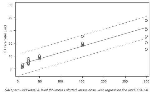
Dose Proportionality This examines the data from the SAD part of the study. In this article, only AUCinf is discussed. The dose proportionality of AUCinf is investigated using three different methods: linear model, power model and graphically. Linear Model In the linear model, PK parameters are plotted against the dose, though no logtransformation of the PK parameters was performed. Note: a regression line with a confidence interval (CI) can also be included.

The outcome of the inferential statistical analysis shows that one is not within the 90% CI of the slope (0.75–0.90). Based on this, it can be concluded that AUCinf increases less than dose proportionally over the dose range 10 to 300 mg.

The graph (Figure 2) also includes a reference line in red with a slope equal to one – this highlights that the slope of the PK parameter is lower than one. Although the PK parameter seems to increase in a doseproportional manner, if no reference line is

Figure 1: Dose Proportionality: Linear Model

In the statistical model of the linear model, the PK parameter is the dependent, and the dose administered is the fixed effect. In addition, a quadratic term (dose*dose) can be included to investigate the non-linearity of the effect.

The outcome of the inferential statistical analysis shows a significant (p-value <0.05) dose-effect and a non-significant (p-value >0.05) dose*dose-effect. Based on this, it can be concluded that there is a linear increase in PK parameters with increasing dose, and there is no quadratic effect.

Only use this model to draw conclusions about dose linearity – not about dose proportionality. Power Model The power model can be used to conclude on dose proportionality. In this model, the log-transformed PK parameter is plotted against the log-transformed dose (Figure 2). If the 90% CI of the slope contains one, dose proportionality can be concluded.

The statistical model for the dose proportionality analysis has the logtransformed PK parameter as dependent and the log-transformed dose as a fixed effect. similar. In Figure 3, it’s clearly visible that with higher doses, the dose-normalised PK parameters are lower – thus the PK parameter increases less than dose proportionally.

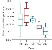
Figure 2: Dose Proportionality: Graphical evaluation: box plot

plotted, it’s not obvious from the graph that the slope is lower than one. Conclusion: Dose Proportionality Analysis We’ve examined three different methods to evaluate dose proportionality: linear model, power model, and a box plot graphical representation.

The models show different conclusions. The linear model clearly shows that AUCinf is increasing in a linear way with increasing the dose. On the other hand, the second

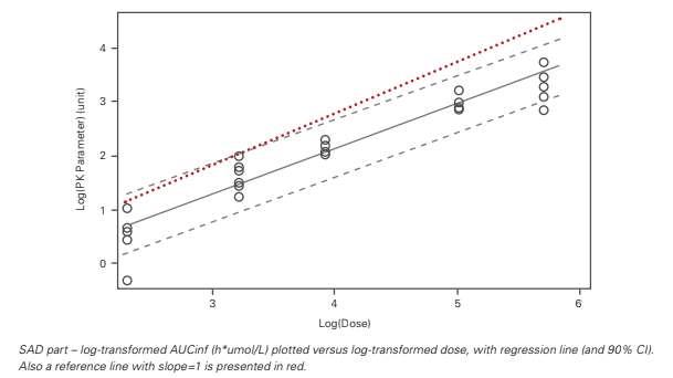
Figure 2: Dose Proportionality: Power Model

Graphical Evaluation The simplest way to evaluate if the PK parameters increase dose proportionally is to plot the dose-normalised parameters in function of the dose. In this article, a box plot is presented (Figure 3), although other types of graphs are also suitable.

Note that the axis with the dose is categorical in these types of graphs.

Dose proportionality can be concluded if the dose-normalised PK parameters are method (power model), shows that this is no dose-proportional increase in AUCinf – rather, that AUCinf increases less than dose proportionally. The simple box plot provides the same conclusion.

The key message is that you need to understand what you plot to draw the correct conclusion: is it a linear or doseproportional increase? For example, we can clearly see that while the data looks nicely scattered in the power model, this doesn’t necessarily mean that there is a dose-

proportional increase in PK parameters. For this to be the case, one would need to be included in the CI of the slope. Steady State The data of the MD part is available, i.e. one cohort with six subjects that received active treatment (daily dose of 300 mg for seven days). For the steady state, the trough concentrations are considered, and it’s investigated using three different methods: linear trend, pairwise comparison, and graphically. Linear Trend Log-transformed trough concentrations are tested in repeated measures ANOVA (Analysis of Variance). Attainment of steady state is determined by stepwise testing for linear trends over successive ranges of days.

Orthogonal polynomial coefficients are used for the contrasts (e.g. Day six to eight: -1 0 1). Steady state can be concluded when the 95% CI of the slope of the day range contains zero.

Based on the results from the ANOVA model (Table 1), steady state is reached by Day three.

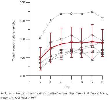
Figure 4: Steady State: GRaphical Evaluation: mean (+/-SD) and individual through concentrations

Since multiple comparisons are done, adjusted p-values are considered. Based on the results from the ANOVA model (Table 2), steady state is reached by Day four.

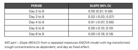
Table 1: Steady State: Linear Trend

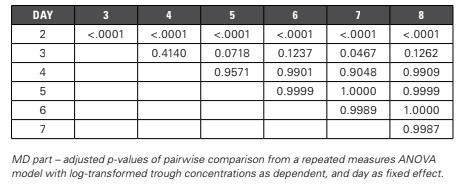
Table 2: Steady State: Pairwise Comparison

Pairwise Comparison Alternatively, you could use pairwise comparison to conclude on steady state between days. When comparing trough concentrations day by day, steady state achievement can be concluded when there is no longer a significant difference between the days. Graphical Evaluation Lastly, steady state can also be evaluated using a graphical presentation of the trough concentrations in function of the day (Figure 4). Steady state achievement can be concluded when the trough concentrations are practically stable. Based on the mean profile, steady state is reached by Day four. Conclusion: Steady State Analysis For the steady state assessment, three different methods are discussed. Based on the first method (linear trend), steady state is reached by Day three. The second method (pairwise comparisons) shows that steady state is reached by Day four. The same conclusion could be drawn from the graphical presentation.

The first two methods require intensive SAS programming. The latter method, a simple plot, has a more subjective way of drawing a conclusion. Nevertheless, a similar estimate on steady state achievement can be taken as with the inferential statistical methods described above. Food Effect The food effect is evaluated in one cohort (Cohort four -150 mg) of the SAD part. In this cohort, six subjects received the treatment in a fed or fasted state following a two-way crossover regimen. In this article, however, only AUCinf is discussed.

The food effect of AUCinf is investigated using both inferential statistical analysis and a graphical evaluation. Inferential Statistical Models Two different inferential statistical models are tested. The first is described in the protocol by client and included treatment as fixed effect and subject as random effect (Model A).

The second model followed the FDA guidance1, including treatment, period, sequence and subject nested within sequence as fixed effects (Model B).

The outcome of both models is quite similar (Table 3). Graphical Evaluation Just as before, the food effect can also easily be evaluated using graphs (Figure 5). Here, two types of graphs are proposed. In the first graph, mean (+/- SD) and individual data are presented versus the food condition (fasted or fed), with different symbols assigned

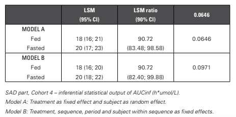
Table 3: Food effect: Inferential Statistical Models

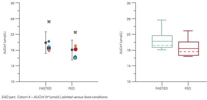
Figure 5: Food Effect: Graphical Evaluation: mean (+/-SD) and individual data and boxplot

The LSM and LSM ratio are similar, with minor differences in the CI. The p-values are not discussed as the study is not powered to perform this food effect.

The results of the food effect also demonstrate the importance of the correct interpretation of the results. Solely based on the LSM ratio, one can conclude that there is a statistically significant food effect, given that 100% is not included in the LSM ratio CI.

Although this may be true, the LSM ratio is about 91% and thus this is not a clinically relevant decrease. It’s better to instead consider the bioequivalence limits, i.e. that 90% CI of the LSM ratio should fall within 80 to 125%. Based on this, it can be concluded that there is no difference between administration under fed or fasted conditions. per subject. In the second one, the data is presented in a box plot.

We could conclude a significant effect from the food conditions if there were no (or limited) overlap between the treatment data. In both graphs, however, the two food conditions still overlap – meaning there's no impact on the food conditions. Conclusion: Food Effect Analysis For the food effect analysis, both inferential statistical methods and the graphical evaluation gave a similar outcome. Conclusion This article explored different statistical analysis methods for pharmacokinetic data in FIH studies. It delved into the importance of preparing properly – of making sure to develop a detailed statistical analysis plan and to review the data thoroughly to potentially exclude unreliable or unexpected results prior to starting with the analysis. It then went on to explore graphical presentation and clearly outlined why inferential analyses should only be thought of as exploratory. REFERENCES

1. FDA guidance “Food-Effect Bioavailability and Fed Bioequivalence Studies”

Joanna Magielse

After completing her PhD in Pharmaceutical Sciences at the University of Antwerp (Belgium), Joanna Magielse started working at SGS as Pharmacokineticist in 2012. Over the years, pharmacokinetic knowledge has been gathered and now, Joanna leads the pharmacokinetics team as Team Manager Pharmacokinetics. The SGS Pharmacokinetics team has a wide range of experience in Phase I clinical trials. Joanna and her team have presented various pharmacokinetic related topics at PhUSE and CDISC conferences over the past years.