Optimising Glulam Structures

OPTIMISING GLULAM STRUCTURES

COMPUTING TIMBER BIFURCATION SYSTEMS FOR FUNICULAR TYPOLOGIES

SVENJA SIEVER

UNIT PG 14

MARCH THESIS 2021/2022

ACKNOWLEDGEMENTS

Thesis Tutor

Tim Lucas (Price and Myers / Bartlett)

Module Coordinators

Oliver Wilton (Bartlett)

Robin Wilson (Bartlett)

Stephannie Fell Contreras (Bartlett)

PG 14 Tutors

Dirk Krolikowski (DKFS / Bartlett)

Jakub Klaska (ZHA / Bartlett)

Structural Engineers

Damian Eley (Expidition Engineering)

Florian Gauss (Knippershelbig)

Advice and Support

Fellow PG14 students

(Special thanks to Chenru Sung, Vegard Elseth, Kacper Pach)

OPTIMISING GLULAM STRUCTURES

ABSTRACT

Wood performs best along the grain, making bending timber more resource-efficient, durable and structurally effective than cutting it. Therefore, this design thesis will investigate glulam construction and the opportunities for resource-efficient building through parallel-to grain bending. It proposes a computational workflow for projecting an optimised glulam bifurcation system onto free-form funicular structures for optimal force transmission. This workflow includes particle-spring form-finding and structure system generation through computer-aided design (CAD) tools.

The thesis is divided into 3 Sections: Glulam History and Development, Computational Experiments and Design Studio Project Synthesis.

Section 1 delineates the evolution and milestones of composite timber construction through the investigation of historical case studies. The current digital shift towards CAD enables file-to-factory workflows and the associated opportunities for mass customisation.

Section 2 focuses on digital experiments and fabrication and executes the established workflow for glulam projection onto funicular shapes, starting from perimeter definition to wood species selection.

Section 3 focuses on applying the learning outcomes to the studio design project.

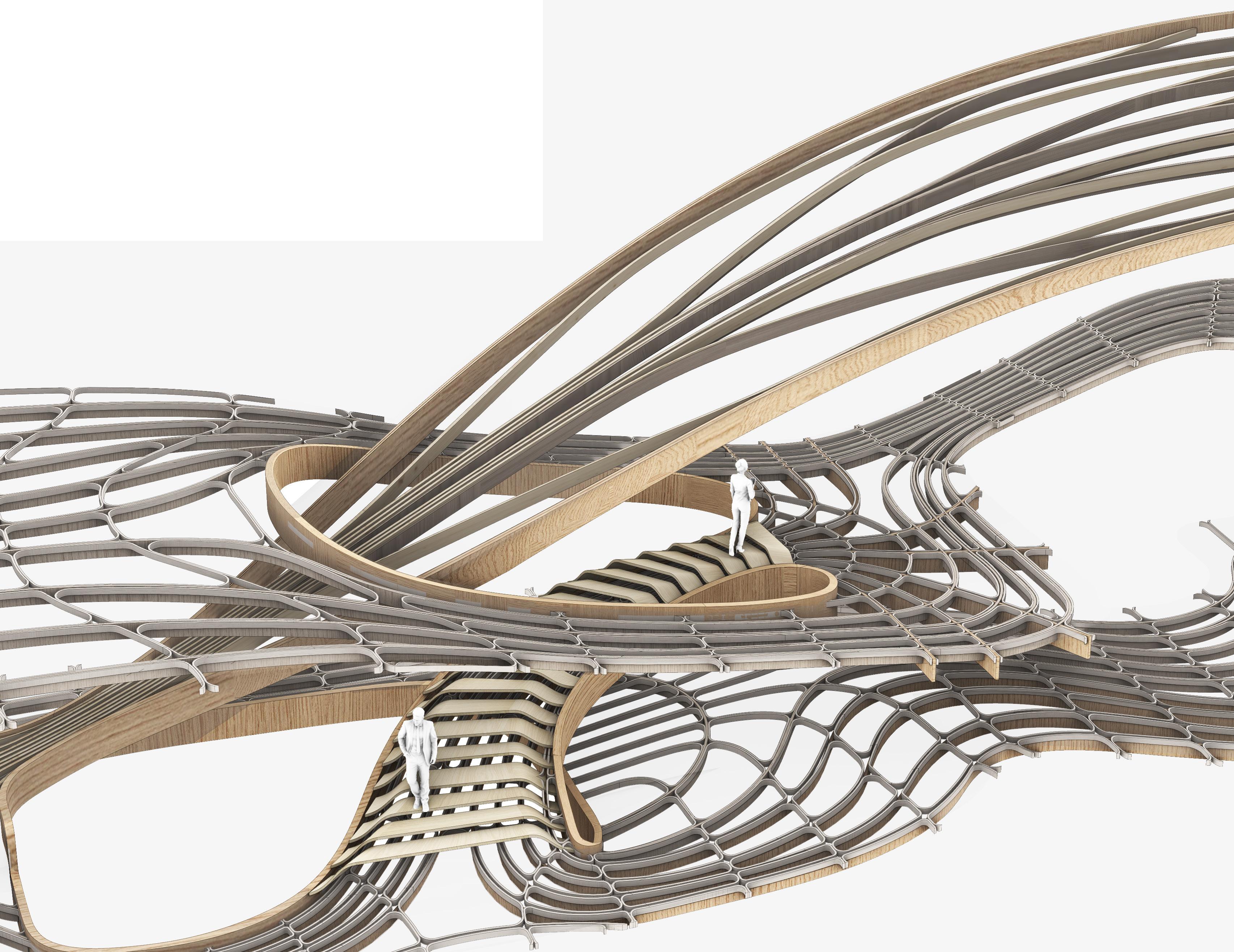
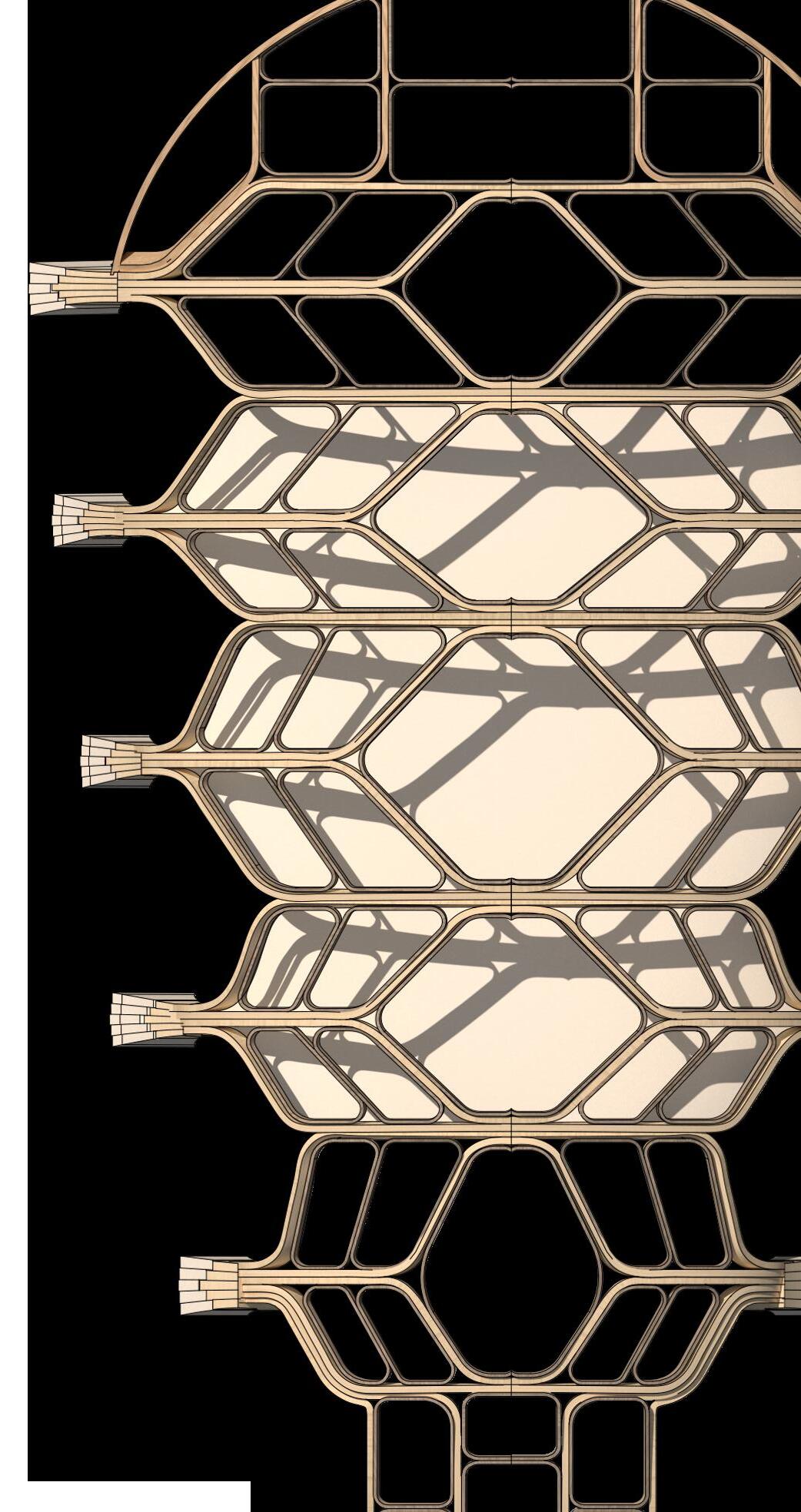
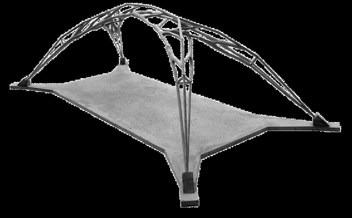
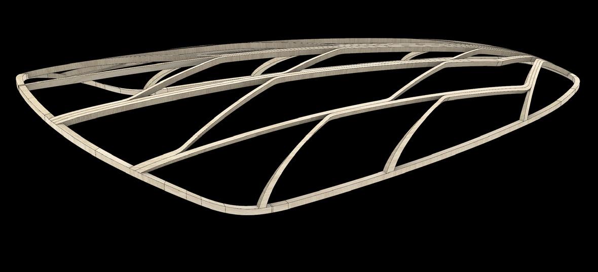
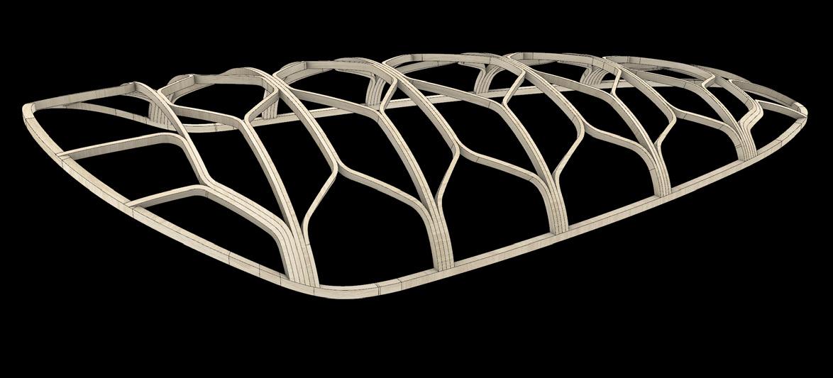
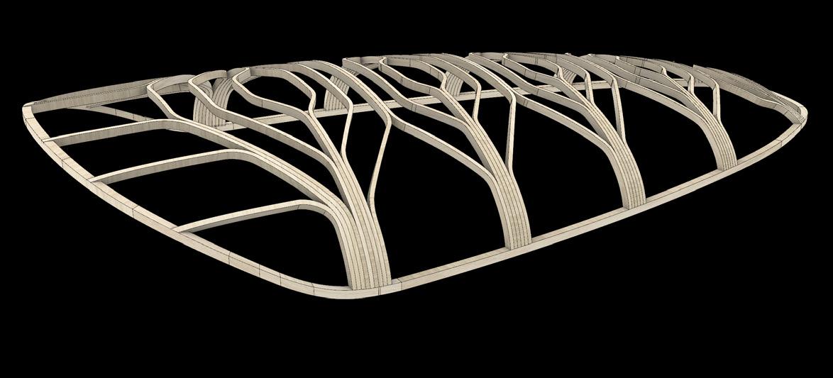
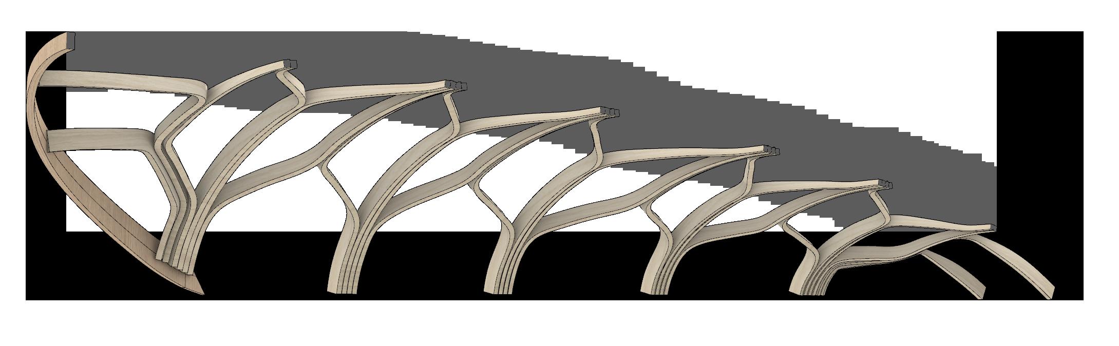
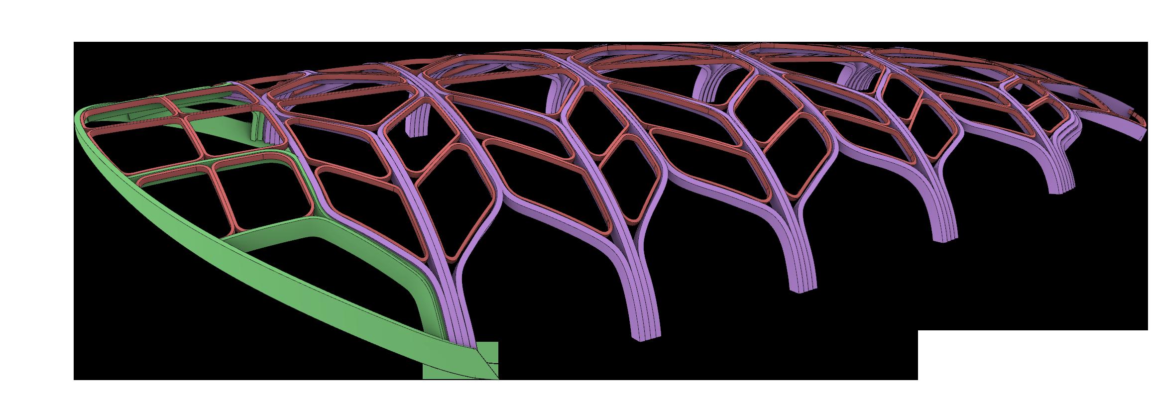
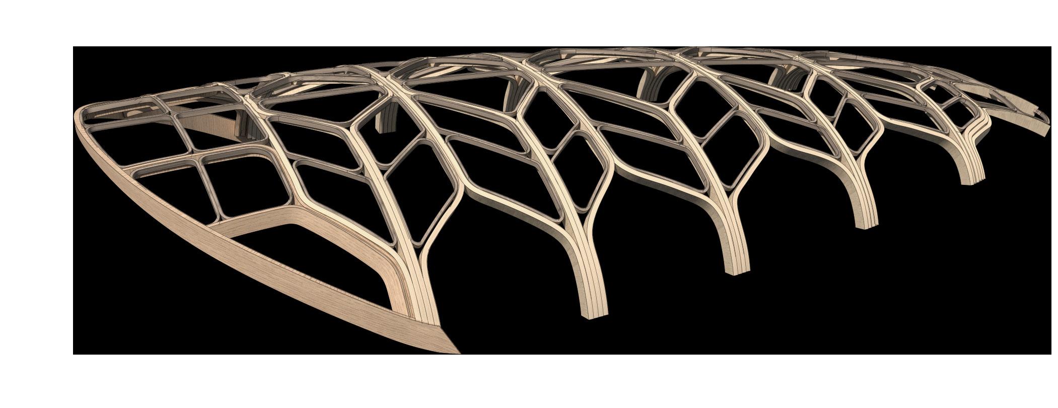
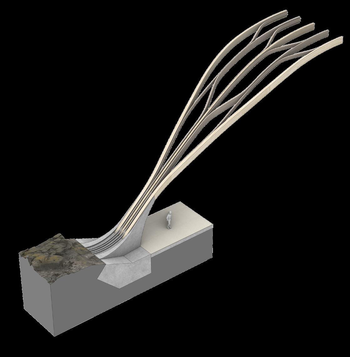
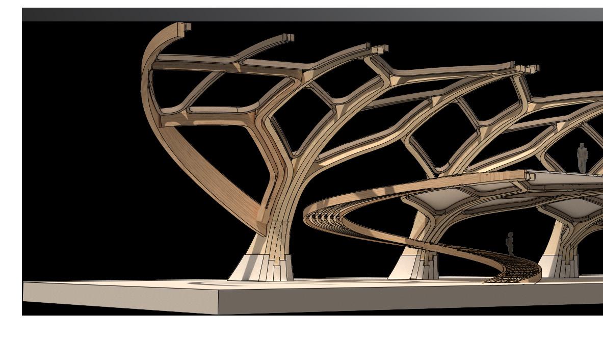
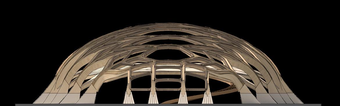
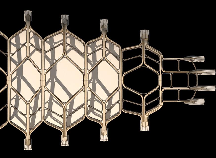
Fig. 1a, b Title Page (Title Page, Left) Bifurcated glulam structure projected onto continuous surface

Glulam History and Development

1.2.2 Bolt-Laminated Timber: Armand-Rose Emy

The industrial revolution in the nineteenth century brought about profound changes in society and technology. Large industrial buildings were in high demand, and roof structures had to span greater distances. Machine-driven saws and mass-produced nails and bolts were developed, significantly lowering costs and making truss assembly easier. New technologies for timber composites were investigated in order to compete with steel. This development resulted in the invention of laminated timber (Toussant, 2007).

Convinced of the advantages of De l’Orme’s method, French Colonel Armand-Rose Emy (1771-1851) was one of the first engineers who used laminated timber instead of short pieces of wood, which he illustrates in his publication Description d’un nouveau system d’arcs (Müller, 2000).

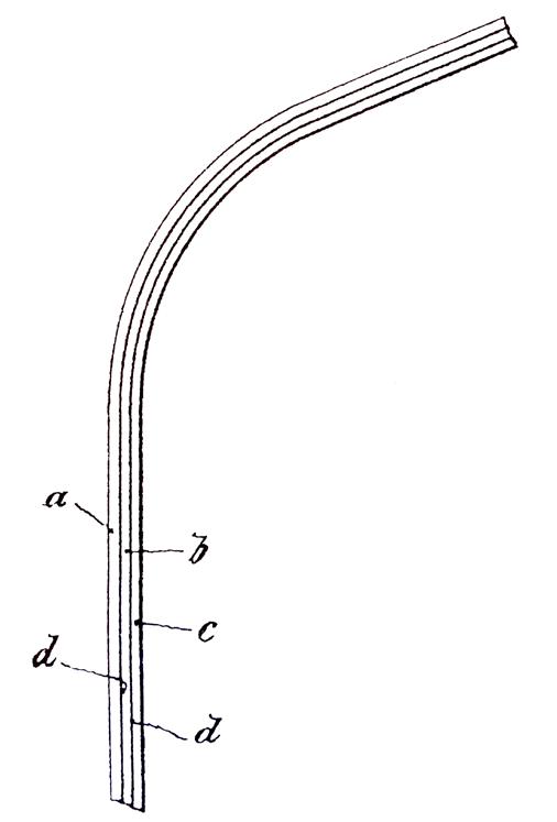
The fundamental difference between the Emy method (Fig. 1.6), which was invented around 1830, and Philibert de L’Orme’s system is that Emy’s invention uses stacked laminations that are glued together and bent, whereas De L’Orme uses vertical laminations (Jeska and Pascha, 2014).

The various layers were joined using clamping bolts and collars to increase friction between the laminations and transfer forces between the layers (Müller, 2000). The Emy approach aligned the timber with the arch’s ideal stress line, reducing the need for additional outside edge cutting to suit the curvature (Svilans, 2020).

However, as the splice connections were neither glued nor interlocked, bending and shear loads caused the laminations to be displaced relative to one another. This, along with the low stiffness of the Emy composite members, resulted in deflections under changing load patterns (Müller, 2000, p. 15).

Fig. 1.5 Composite Beam Evolution (Bottom) Chronology of proposals marking the evolution of beam reconstruction

Fig. 1.6 De L’Orme System Detail (Opposite) Multiple curved planks, fixed together with bolts and metal straps

Leonardo Da Vinci 16th Century

Phillibert de L‘Orme 16th Century (1567)

Armand-Rose Emy 19th Century (1837)

Fausto Veranzio 16th Century

Guiseppe Del Rosso 18th Century

Pierre Henri Migneron 19th Century

Karl Friedrich Otto Hetzer 20th Century (1906)

Carl Friedrich Wiebeking 19th Century (1817)

1 Steel collar

2 Timber connection element to roof structure

3 Steel clamping bolts

1.2.3 Glued-Laminated Timber: Karl Friedrich Otto Hetzer

Tests on the first glulam beams were carried out in Karl Friedrich Otto Hetzer’s (1846-1911) firm after 1900 (Müller, 2000). Between 1891 and 1910, Hetzer obtained several patents for a series of improvements aimed at optimising the use of wood in structural elements such as beams and trusses (Svilans, 2020).

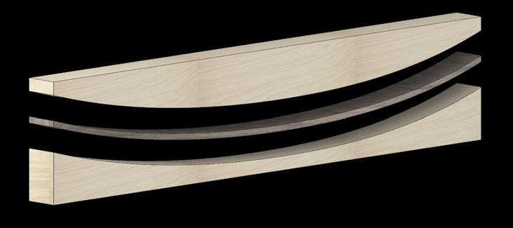
The bending diagram of a simply supported beam was mapped by patent number 125895 (Fig. 1.7), which led to a pair of profiled web components attached between a straight top flange and a curved bottom flange. This was the first time the crosssection of a laminated timber beam was optimised, with the cross-section changing in response to the load (Svilans, 2021).

Patent number 163144 (Fig. 1.10) depicts a spruce beam sawn longitudinally to form a parabola and filled with a pine plank glued into place under pressure. By that, Hetzer tackles the issue of cross-section optimisation and connection via adhesive application (Müller, 2000)

However, the Hetzer beam failed on the underside due to breaking wood fibres, and the saw cut along the length remained a costly manufacturing procedure (Müller, 2000).

The 1906 patent 197773 (Fig. 1.8) replaced mechanical fasteners with adhesives and was designed as a composite component for roof posts and rafters (Svilans, 2020). This patent was a significant turning point in modern glued laminated timber construction since it offered an efficient method for producing curving structures in timber without wastage (Jeska and Pascha, 2014).

Before glueing, individual wood laminations were bent to the desired shape. Hetzer carried the Emy composite member to its logical conclusion, allowing the structure to be closely matched to the ideal pressure line while achieving the highest possible bending strength, thus saving material.

Wooden planks could now be bent and attached to others; the shape was cemented once the adhesive cured. Introducing prestress into the wood fibres increased the structural response (Jeska and Pascha, 2014).

Hetzer’s patents were licensed to other international producers, resulting in the worldwide glulam construction endorsement (Müller, 2000).

Fig. 1.7 Hetzer Patent 125895: Load-Optimised Composite Beam

(Bottom Left) Web element with straight top flange and curved bottom flange

Fig. 1.8 Hetzer Patent 197773: Glued-laminated Timber Beam (Bottom Right) Curved timber member serving as both column and rafter

Fig. 1.9 Hetzer Patent 125895: Composite I-Beam

(Opposite Top Left) Composite beam with harder heartwood in the at the edges and softer sapwood in the middle to match the stresses

Fig. 1.10 Hetzer Patent 163144: Parabolic Composite Beam

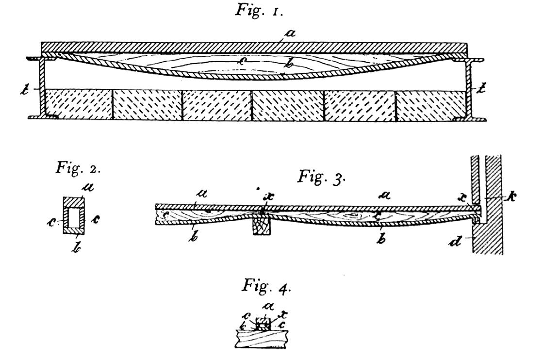
(Opposite Top Right) Composite beam sawn lengthwise to form parabola and complement

Fig. 1.11 Case Study: Doecker Gymnasium Wuppertal 1911

(Opposite Bottom) The dismantable “Doecker system building” inspired by Hetzer’s patents has a supporting structure made of three-hinged laminated timber arches

Heartwood (compression-resistant)

Sap wood

Heartwood (tension-resistant)

1 Bent glued-laminated I-beam 2 Barrel vault louver ceiling 3 Purlin roof system

Solid wood girder (spruce)

40mm pine panel infill along moment path

compression tension compression tension

1.3 The Digital Shift

Computer-Aided Design (CAD)

File-to-Factory

Nowadays, digital tools have permeated all aspects of the designto-production process (Svilans, 2020).

New building construction logic such as the “digital chain,” “design for manufacture and assembly (DfMA),” and “file-tofactory” processes have resulted from the convergence of digital design and digital production, supported by computationallydriven parametric and procedural modelling paradigms (Larsen and Schindler, 2008, p. 399). These workflows refer to a method that involves the direct transfer of data from a 3D modelling programme to a CNC (Computer Numerically Controlled) machine. This process aims to fully utilise digital tools, particularly BIM, which can provide a smooth transition from design to manufacture (Robinson, 2019).

Prefabrication

Prefabrication provides more control, flexibility, and customisation. Buildings can be prototyped and tested before being assembled by moving construction from the site to a controlled environment (Svilans, 2020). This facilitates experimentation and iterative prototyping by experts.

Case Study: Savill Building, 2006

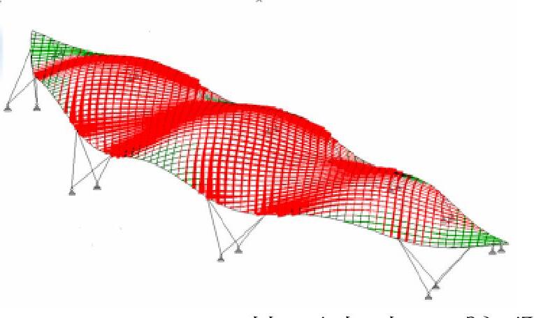
As demonstrated by the Savill Building, varying elements are a distinguishing feature of free-form timber constructions, made possible only through the digitalisation of the design process (Svilans, 2020). The perimeter is drawn on a plan using arcs formed by two intersecting circles (Fig. 1.12). A sine curve generates the roof’s centre line with variable amplitude. The cross-section is drawn as a series of parabolic arcs across the centre line. The surface is then covered with a grid generated by a programme that defines the “shape as z = f(x, y) with a damped cosine wave in the x-direction and upside down parabolas in the y-direction” (Harris and Roynon, 2008).

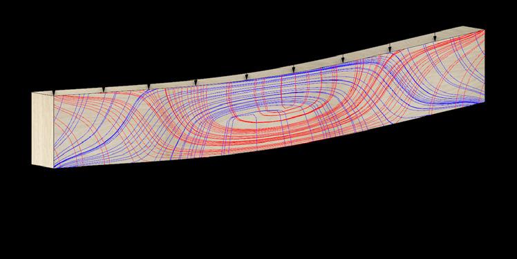
The architects and engineers worked together to fine-tune and settle on a shape that met aesthetic and functional needs (Fig. 1.13). Once the form-finding model was agreed on, it was imported into a structural analysis model. The Robot 3D programme helped determine load concentrations (Fig. 1.14) The model was then sent to the fabricator to detail the structural elements (Harris and Roynon, 2008).

Fig. 1.12 Savill Building Workflow: Digital Perimetre Definition (Top) The perimetre is set out using the arcs of two intersecting circles

Fig. 1.13 Form-Finding and Analysis Model (Middle) Once form-finding is concluded, the model is imported into a structural analysis model

1.4 Understanding Timber Characteristics

1.4.1 Grain Direction and Strength Factors

There are three perpendicular principal orientation axes: longitudinal, radial, and tangential. The ability of wood to withstand weights is affected by several elements, including the kind, direction and duration of loading, defects, moisture, and temperature (Green, 2001).

Defects

Strength-reducing properties can dramatically diminish tensile and compression strength in structural timber (Harte, 2009). Therefore, the given values only apply to clear, straight-grained wood samples.

Moisture and Temperature

Water held in the cell wall is bound water, whereas water held in the free gaps is called free water (Svilans, 2021). The moisture content at which all free water has been eliminated is known as the fibre saturation point (FSP). Changes in FSP moisture content cause the wood to swell or shrink (Fig. 1.18). Softwoods have an equilibrium moisture content of about 12% in a typical indoor climate with a temperature of 20°C and relative humidity of 65%.

Duration of Load

Because wood is a time-based visco-elastic material, bending it for an extended time keeps part of the bent shapes even after eliminating the forces. This is known as creep (Svilans, 2021).

Elastic Properties

The elastic qualities of wood are created under mild stress and are entirely recoverable once the forces are eliminated. The elastic constants and elastic constant ratios vary depending on the species, moisture content, and temperature at which they are tested (Green, 2001).

Fig. 1.16 The Three Primary Axes of Wood (Top) Three principal axes of wood with respect to grain direction and growth rings

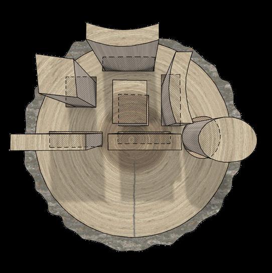
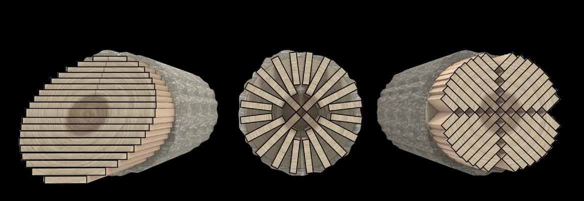
Fig. 1.17 Timber Cuts (Middle) Plain-sawn, rift-sawn and quarter-sawn timber logs are subjected differently to shrinkage

Fig. 1.18 Distortion of wood due to shrinkage and swelling (Bottom) Depending on shape and the location of the cut, the lumber warpes differently

Mechanical Properties

Plastic deformation or failure occurs when the timber is “loaded to higher stress levels beyond the elastic range” (Green, 2001, p. 9732).

• Compressive strength indicates how much load a wood species will support parallel to the grain.

• Bending strength shows the forces wood can withstand perpendicular to the grain (Engler, 2007).

• Shear strength is characterised by three types of failure: shear parallel to the grain, shear perpendicular to the grain and rolling shear (Harte, 2009).

• Flexural strength illustrates the compression in the top half of a bent timber beam and tension in the bottom half.

Grain Direction

Wood cells are formed of lignin-bound long, strong cellulose fibres. As a result, splitting a board along the grain is significantly easier than breaking it across the grain (Engler, 2007). Therefore, wood can be ten times stronger than across the grain (Fig. 1.19) (Svilans, 2021).

Parallel-to-grain Properties

From a structural standpoint, the parallel-to-grain direction is the strongest and stiffest. Softwood tensile strength parallel to grain typically ranges between 70 and 140 MPa (bending strength). The compression strength is typically 30–60 MPa. These values are often greater for hardwoods (Harte, 2009, p. 710).

Perpendicular-to-grain Properties

The equivalent parallel-to-grain properties are much lower than the perpendicular-to-grain values. Tensile strength in the radial and tangential directions can be as low as 5–8 per cent and 3–5 per cent of the values in the grain direction, respectively. Compressive strengths perpendicular to grain are around 10–20% of parallel-tograin values (Harte, 2009, pp. 710-711).

Fig. 1.19 Hankinson’s Equasion

(Top) Relationship between wood grain orientation and the compressive/tensile strength of wood

Fig. 1.20 Timber Load Behaviour Parallel and Perpendicular to Grain

(Bottom) Mechanical Properties: Tension, Compression, Shear and Bending

Sliding Kinking Rolling Flexual

1.4.2 Glulam Blank Types and Lamella Assembly

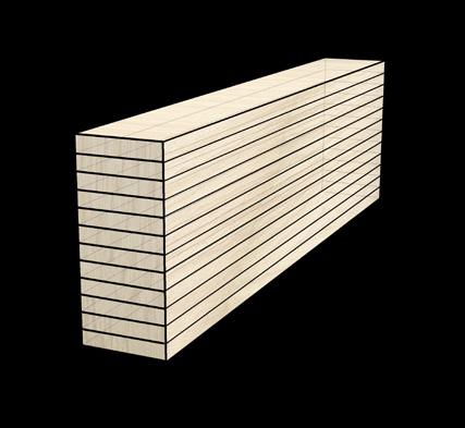
Straight glulam blank

Straight glulams are the easiest blanks to fabricate. Straight glulams are typically constructed by vertically stacking dimensioned lumber to produce the appropriate depth (Svilans, 2020, pp. 95-96).

Single-curved glulam blank

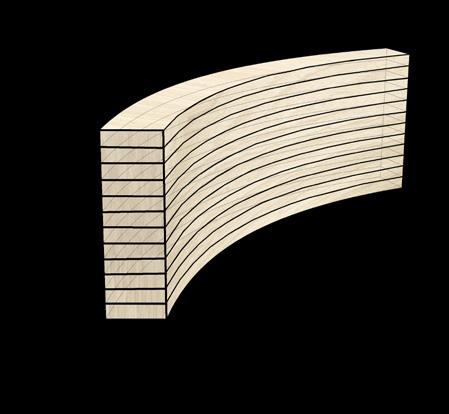
Single-curved glulams are curved in-plane. The timber boards are arranged so that their shortest dimension faces the curvature direction. Single-curved glulam production is more complex than straight glulam production due to the usage of a curved press (Svilans, 2020).

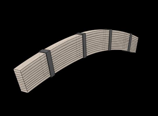
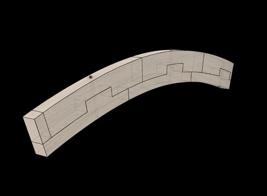
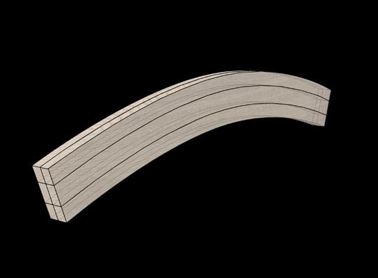
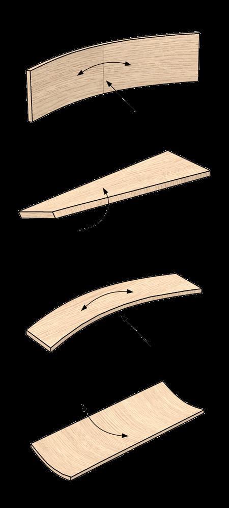
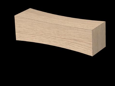
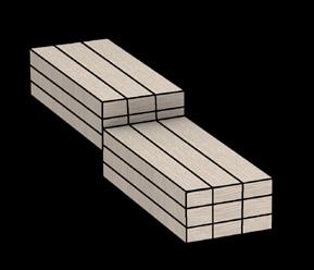
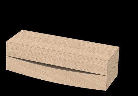
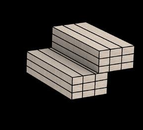
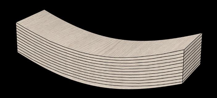
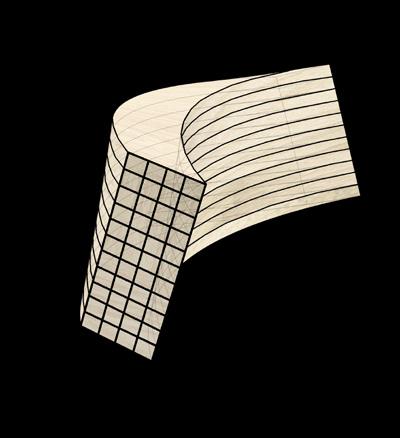
Double-curved glulam blank

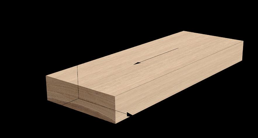
The degree of curvature in out-of-plane glulams influences the lamellae’ width and thickness. The beam is constructed using a multi-axis glulam press; it is first created as a single-curved blank before being cut into parallel slices. In a subsequent production step, it is twisted out of plane (Svilans, 2020) (Fig. 1.21)

Lamella Assembly

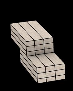
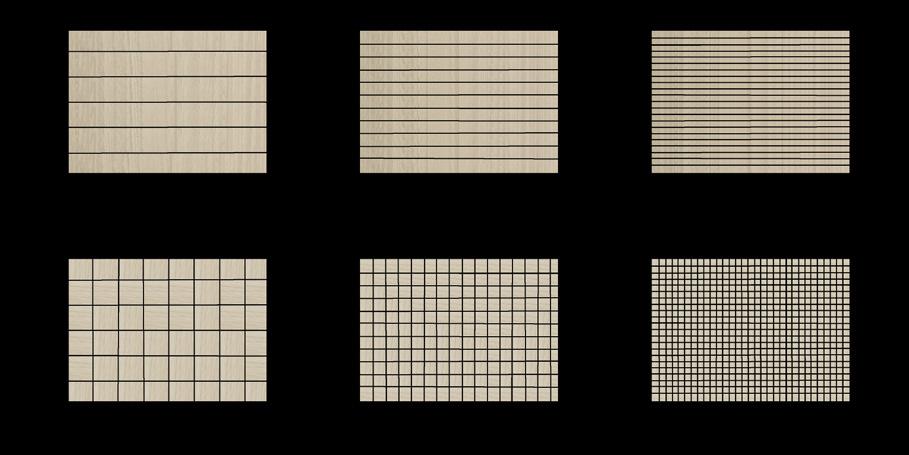
Thinner wood elements can be bent with less force. Therefore, the thinner the lamellae, the more a glulam beam can be bent (Fig. 1.22). Using more layers of lamellae increases the amount of glue surface.

This thesis will focus on finding a bifurcation system for shell structures that minimises the application of double-curved elements, as the fabrication is complex and expensive. This will be further investigated with an example model in Section 2.

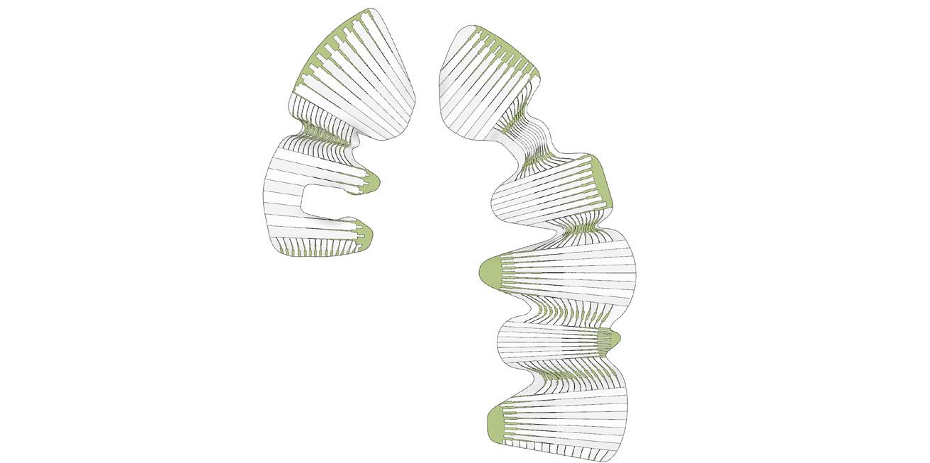
Fig. 1.21 Types of Glulam Blanks (Bottom Left) Glulam beams can be bent in one or two directions

Timber Beam Single-Curved Double-Curved Low Curvature High Curvature

2.2.2 Inverted Catenary Framing - Case Studies

Since this thesis focuses on projecting glulam bifurcation systems onto shells, the behaviour of the chords inside the system is critical, as they will reflect the respective glulam beam structure in later tests.

As Isler’s cloth simulation is more applicable for thin concrete shells, this subsection examines two case studies that exclusively used hanging chain form-finding methods to generate skeletal structures.

Woodchip Barn - Catenary Arch Framing

The structure of the woodchip barn in Hooke Park (Fig. 2.6) was created by ‘shuffling’ between available component geometries and using an equilibrium method to align elements optimally. This process is conceived in which natural tree junctions can be reconfigured into architectural structures without needing complex connection hardware. The concept was investigated during the design and erection of the barn by Design & Make students in late 2015 (Menges, 2017). After discussions with the engineering team, the structural form was established to have the necessary invertedcatenary shape for a compression structure and a crosssectional geometry that could support the dimensions and angles of the sourced tree forks (Self, 2017).

Magazzini Generali - Inverted Arch Framing

Inspired by his bridge designs, Robert Maillart (18721940) envisioned the primary frame of the Magazzini Generali warehouse as a narrow inverted arch connected to a rigid ribbed slab using slender vertical links (Fig. 2.7). The idea evolved from the deck-stiffened arch bridge concept: the inverted arch is a concrete prism in tension rather than a curved slab in compression (Billington, 1997). Maillart’s analysis methods were primarily based on graphical computations (Fig. 2.6) The architect was familiar with Gaudí’s designs through visits to his Barcelona office and, therefore, applied his knowledge about funicular structures to the Chiasso project.

Fig. 2.6 Case Study: Woodchip Barn Hooke Park, AA Design+Make, 2016 (Top) Selection of naturally grown bifurcated tree branches, which are structurally composed so the grain direction follows the ideal line of pressure

Fig. 2.7 Case Study: Magazzini Generali Chiasso, Robert Maillart, 1925 (Bottom) The structural form of the arching truss has the inverted-catenary forn for a compression structure and a cross-sectional geometry accommodating the sources tree forks

2.4 Digital Workflow Establishment

Perimeter Definition

Funicular Form-Finding

Gridshell

Workflow Objectives

The suggested workflow proposes learning by discovery through the support of computational tools (Fig. 2.10). The architect can directly view the spectrum of structural responses while exploring various forms, which fosters unusual solutions adapted to the design objectives and encourages an exploratory approach.

However, the design goal is not solely driven by ideal structural shapes. Structural and dimensional analyses are also included. The proposed workflow allows for the iterative back and forth between design decisions and structural response. Variable degrees of optimisation enables the architect to be less efficient, facilitating the incorporation of non-funicular slabs and circulation. The structural system can then be adapted accordingly.

Therefore, the workflow includes form-finding through funicular surfaces, which can be manipulated according to design needs. Different bifurcation systems are projected onto the surface and structurally tested, catering to varying load conditions. The system with the best overall structural and aesthetic performance for each iteration is selected and developed further.

Fig. 2.10 Digital Workflow Proposal

This diagram illustrates the design approach with the support of digital tools

2.5 Computational Funicular Form-Finding

2.5.1 Perimeter Definition

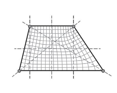
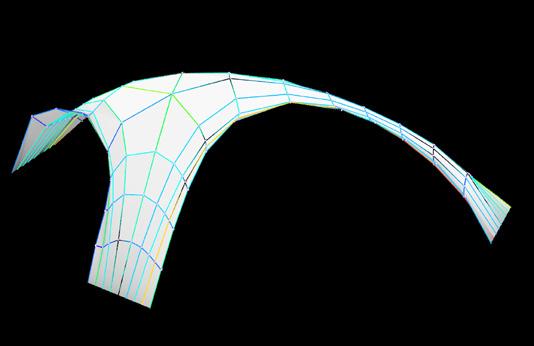
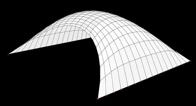
The boundary definition is a purely aesthetic choice. It is entirely up to the designer to determine the perimeter according to their specifications and restrictions. A Conoid Shell structure is used to demonstrate the workflow for demonstration purposes. The Conoid Shell is a simplified model of the design studio project, which will be examined in detail in Section 3.

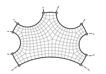
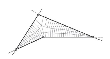
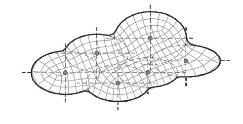
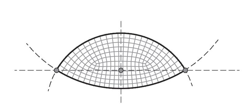
Like the Savill Building case study, the perimeter is defined by two intersecting ellipses that characterise the Conoid Shell’s footprint.

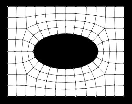
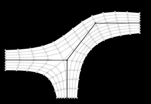
A surface is generated from the boundary curve and subdivided to start the live physics simulation (Fig. 2.12)

For this proceidure, RhinoVAULT 2.0 is used instead of Kangaroo 2, as it provides an intuitive funicular form-finding method independent from additional modelling tools such as Grasshopper. Features, such as mesh subdivisions, reciprocal diagrams and a few analysis options, are integrated into the plugin, simplifying the design process.

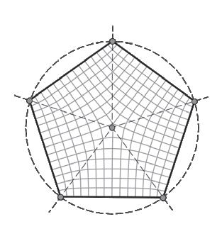
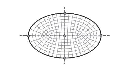
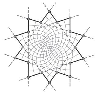
Fig. 2.11 Basic and Complex Shape Boundaries (Top) Selection of basic and complex boundary condition examples

Fig. 2.12 Project Perimeter (Bottom) Boundary condition generation adapted to the project

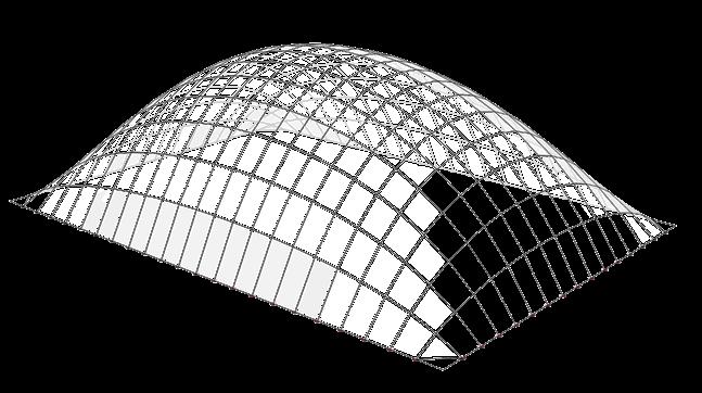
2.5.2 Pattern Generation (RhinoVAULT 2.0)

Pattern Vertical Equilibrium

Pattern From Surface (QuadMesh)

Pattern From Features (QuadMesh)

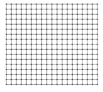
As mentioned in the workflow objectives, form-finding will be done with funicular surfaces on which bifurcation systems will be projected.

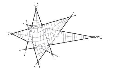
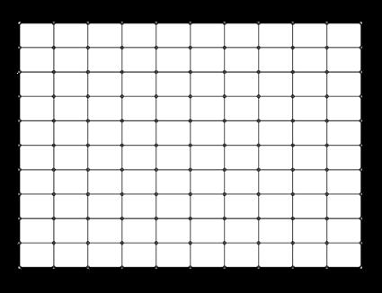
To run the simulation, the example surface needs to be subdivided first. Mesh Patterns in RV2 can be generated from surfaces or lines (Fig. 2.13). A Pattern describes the topology of the FormDiagram. It comprises a series of vertices linked together by lines or edges. RV2 has several tools for modifying and refining a Pattern’s geometry (Block Research Group, 2022).

Pattern From Triangulation (TriMesh)

Pattern From Skeleton (QuadMesh)

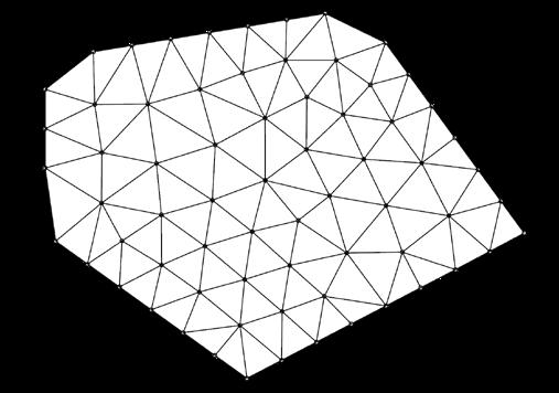
The unstructured TriMesh is simple to generate, and it comes in handy when the boundary conditions are very irregular. Triangulation quickly generates a pattern that helps to dive into form-finding immediately. However, TriMeshes are not suitable for complex schemes. In contrast, a structured QuadMap is more accurate for complex simulation, as often domains need to be partitioned. It is capable of producing better outcomes at higherorder schemes while maintaining numerical stability and accuracy.

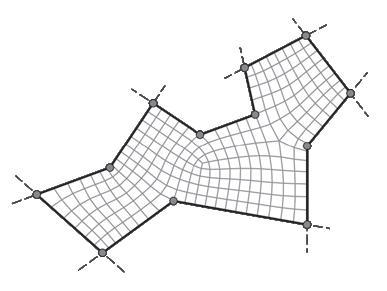
The PatternFromFeatures attribute in RV2 is the most applicable to the Conoid Shell project, as the QuadMesh adapts well to the perimeter and boundary conditions (Fig. 2.14)

Fig. 2.13 RhinoVAULT2.0 Meshing options (Top) (1) Mesh from Surface, (2) Mesh from Triangulation, (3) Mesh from Features, (4) Mesh from Skeleton

Fig. 2.14 Project Meshing (Bottom) QuadMesh pattern generated through Mesh from Features

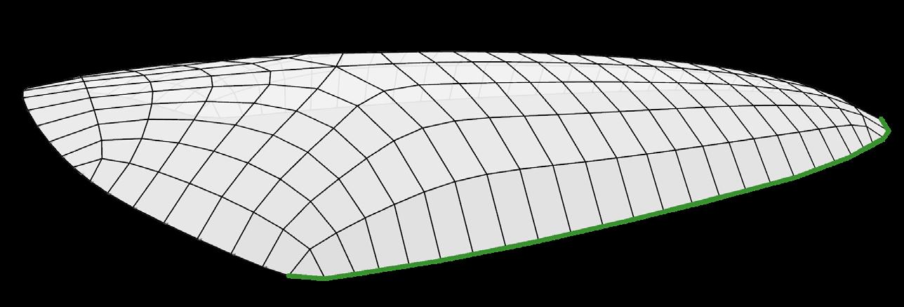
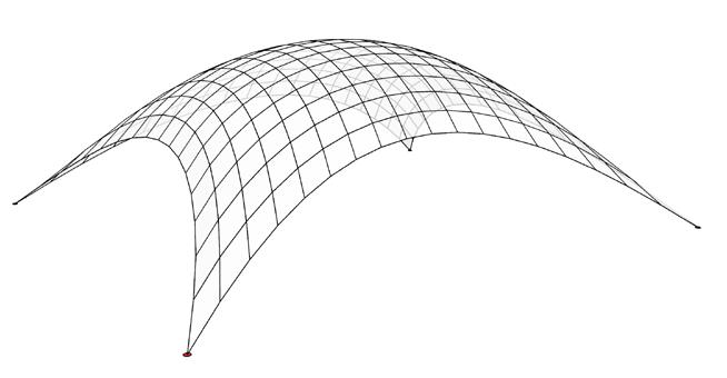
2.5.3 Support Definition

Boundary

Supports

After the generation of the Pattern, further information is added, such as the identification of support vertices and refinement of the geometry of the unsupported boundaries. Refinement includes the Sag option, which relaxes the Pattern.

In the drop-down menu, select Define Boundary Conditions > Define Boundary Conditions > Identify Supports

RV2 includes four support selection options: AllBoundaryVerticies, ByContinuousEdges, Corners, Manual (Fig. 2.15)

The Conoid Shell Project has a cantilever, and therefore, ByContinuousEdges is used for anchor point selection. Once the edge is set, all the vertices along that boundary from corner to corner will be automatically selected (Fig. 2.16)

Boundary conditions --> Select ByContinuousEdges

Fig. 2.15 Anchor Point Definition Options (RhinoVAULT 2.0) (Top) All boundaries, continuous edges, corners

Fig. 2.16 Project Supports (Bottom) All continuous edges serve as supports, with exception of the cantilever

2.6 Conoid Shell Analysis

Pipe Diagram (RhinoVAULT2)

Several features facilitate analysis and enhance 3D visualisation in the ThursutObject Settings

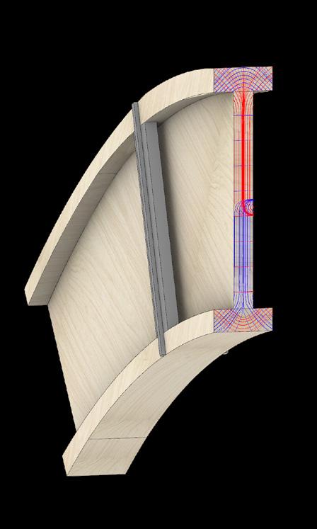
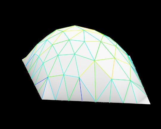
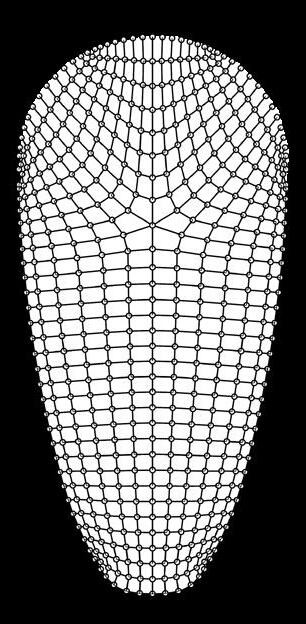
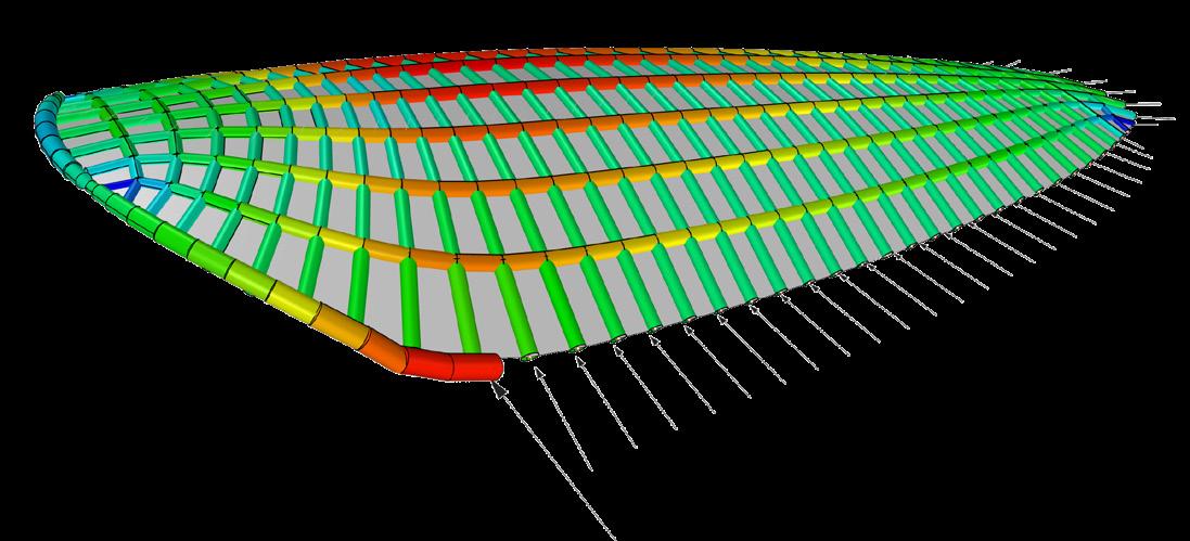
When the ShowColourAnalysis function is enabled, a colour scheme depicts the magnitude of forces in proportion to the model size. With Display Pipes, the boundaries of the ThrustDiagram can be displayed with pipes, the diameters of which are proportionate to the internal forces (Fig. 2.24). The pipe diameter can be adjusted according to the scale of the form diagram. The force-dependent pipe network visualises the force distribution and can help to determine the material distribution of the glulam beam cross-sections in later steps.

Using Karamba for Accurate Shell Analysis

Since precise analysis options are limited in RV2, stresses are also assessed with the help of the structural engineering programme Karamba3D. Karamba accurately analyses spatial trusses, frames, and shells, and it is fully integrated into the Grasshopper and Rhino design environments (Karamba 3D, 2022). The workflow of setting up the model for Karamba analysis is similar to RV2, in which the shell surface, load and anchor points are defined. The results are displayed in the ShellView mode.

It is crucial to recognise that Karamba3D is not a formfinding device but rather a tool to analyse and optimise an already established design idea.

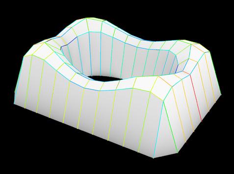
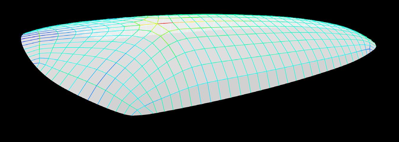
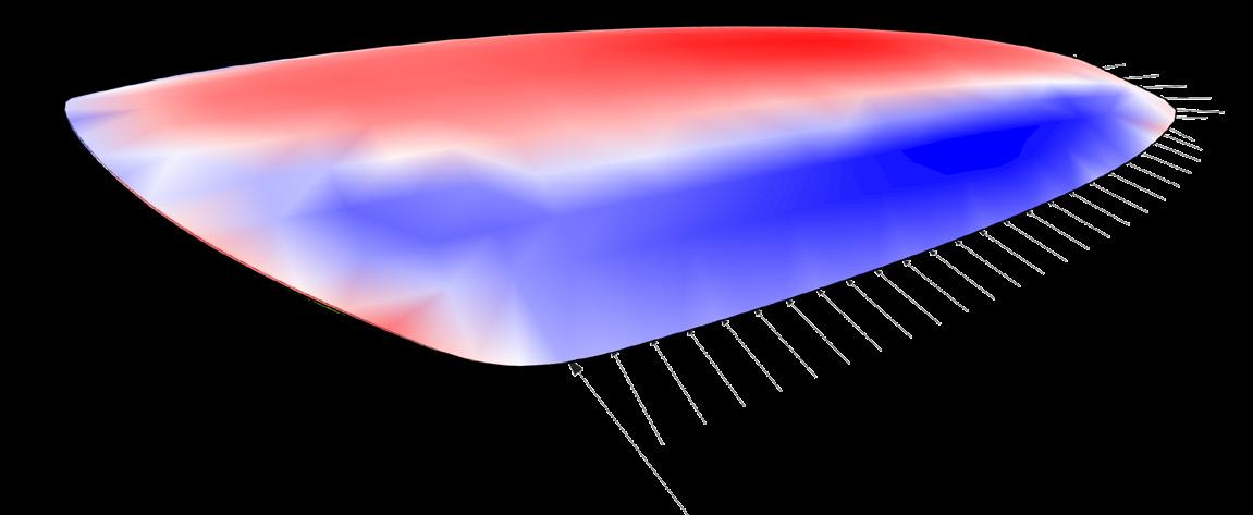
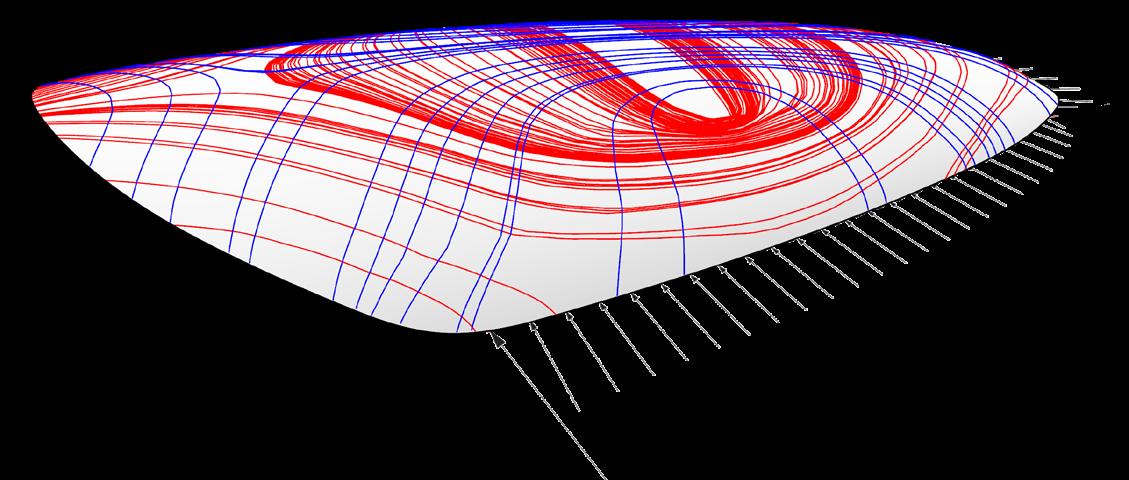
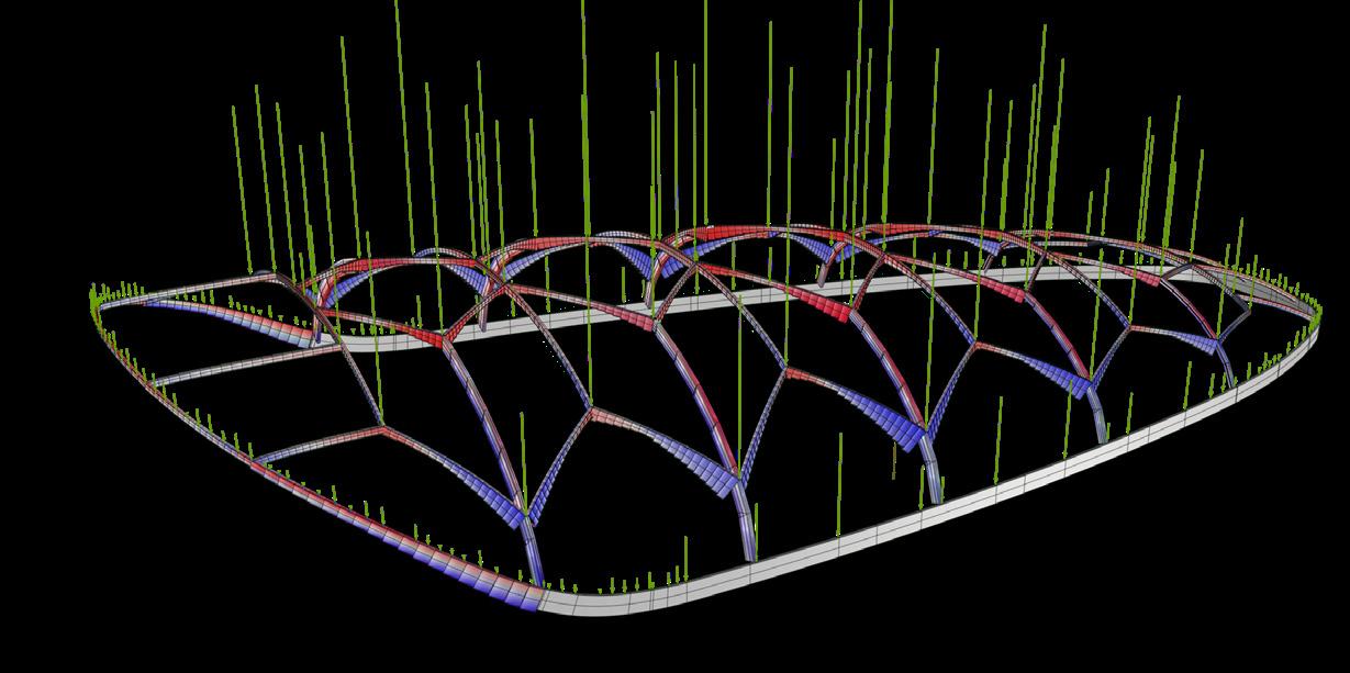
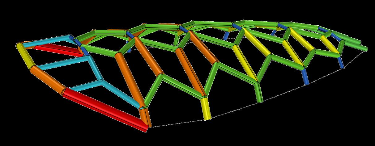
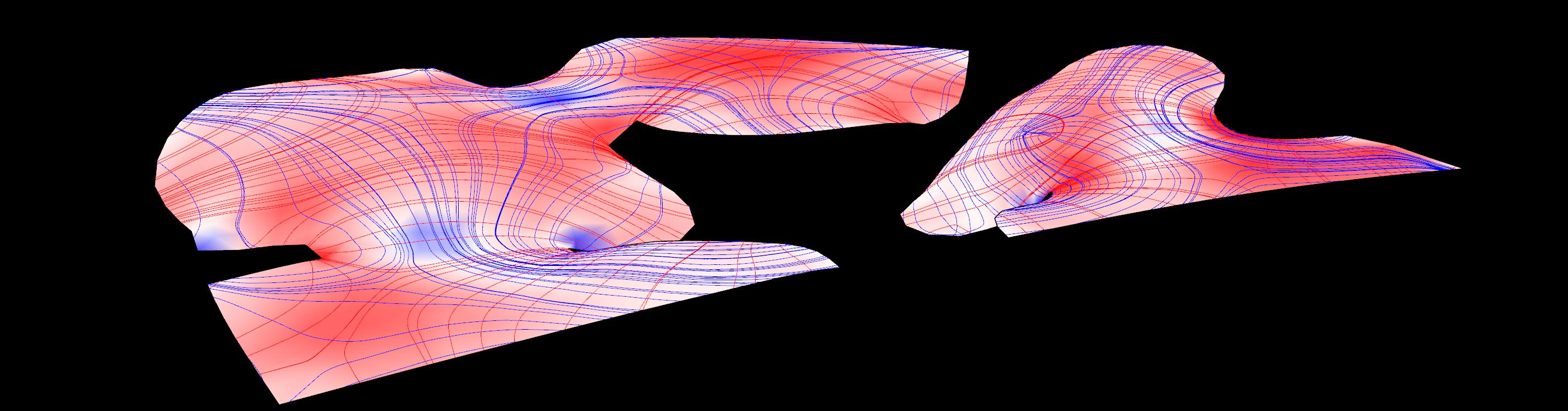
Utilisation and Stress Lines (Karamba3D)

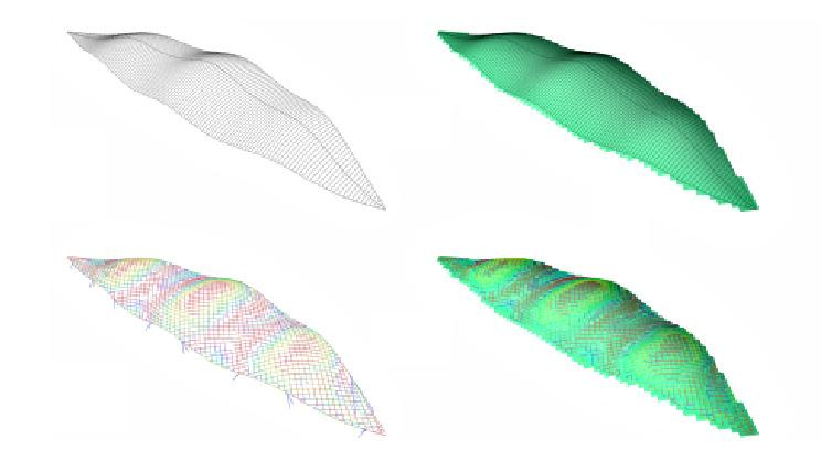
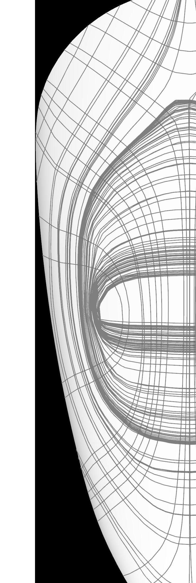
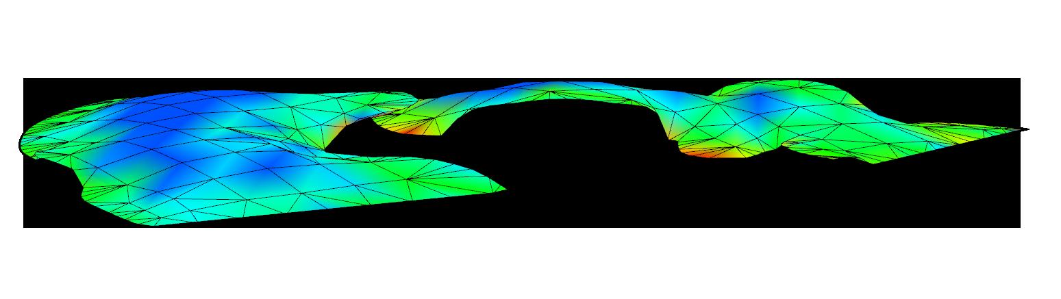
The Utilization displays the axial force causing either tension or compression. The Conoid Shell example shows that the structure experiences compression around the shell’s vertex and the cantilever edges and tension around the supported perimeter (Fig. 2.25a). Internal force trajectories are indicated by principal Stress Lines, which are pairs of orthogonal curves. Subsequently, the curves idealise material continuity paths and represent the best topology for every structure, given a set of boundary conditions (Kam-Ming, 2015). The stress-line analysis provides a direct and geometrically provocative approach to optimisation, synthesising design and structural goals (Fig. 2.25b)

Fig. 2.24 Pipe Diagram (RhinoVAULT 2.0) (Top) Pipe material distribution of form diagram proportional to model size

Fig. 2.25a,b Stress Analysis (Karamba3D) (Bottom) Tension and compression visualised through utilisation (a) and principle stress lines (b)

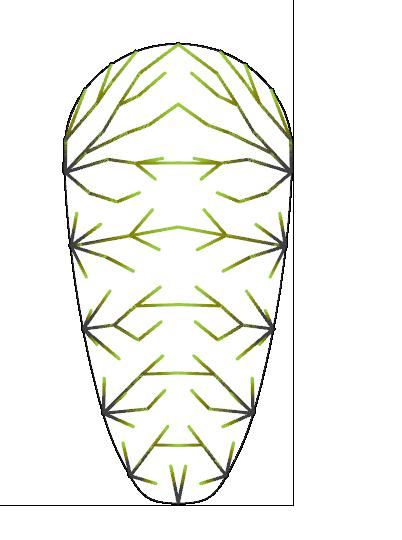
2.7.3 Branching Typology (Lindenmayer-System)

The Lindenmayer-System

Aristid Lindenmayer (1925–1989) presented the L-System mathematical formalism in 1968 as a framework for an axiomatic theory of biological development. Two significant fields are first, the production of fractals and secondly, the accurate modelling of plants. The concept of rewriting is vital to L-Systems. Rewriting, in general, is a method of defining complicated objects by replacing elements of a simple beginning object with a collection of rewriting rules or productions (Fig. 2.28) (Prusinkiewicz and Lindenmayer, 1990). Branching denotes a diverging fork in organic, tree-like structures. In his work, Lindenmayer proposed using strings with brackets to express graph-theoretic trees (Fig. 2.29). The goal was to use the L-System’s framework to properly characterise branching structures found in nature (Ochoa, 1998).

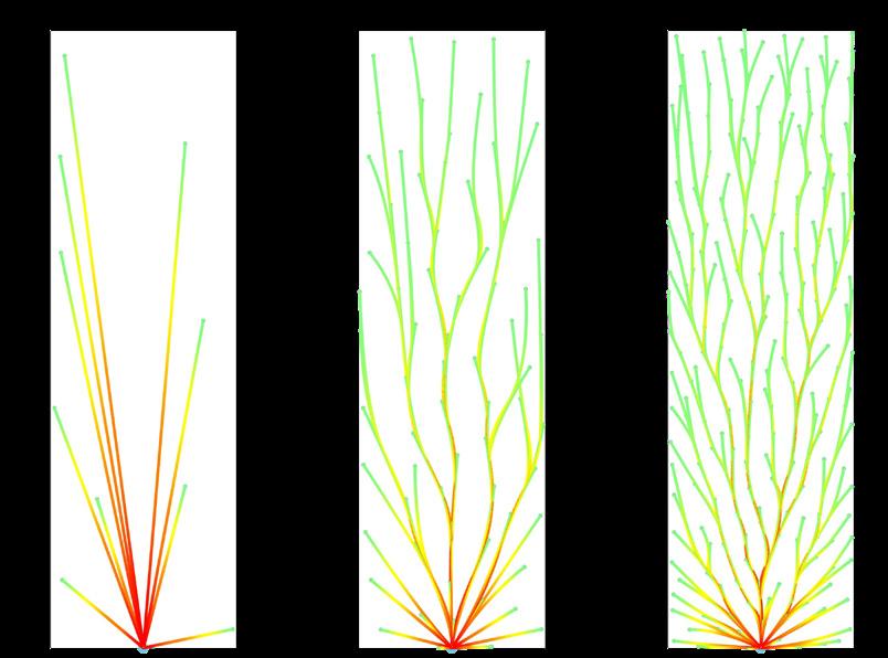
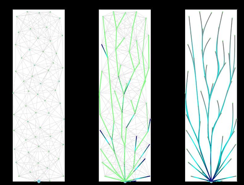
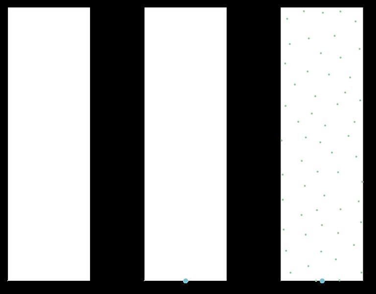
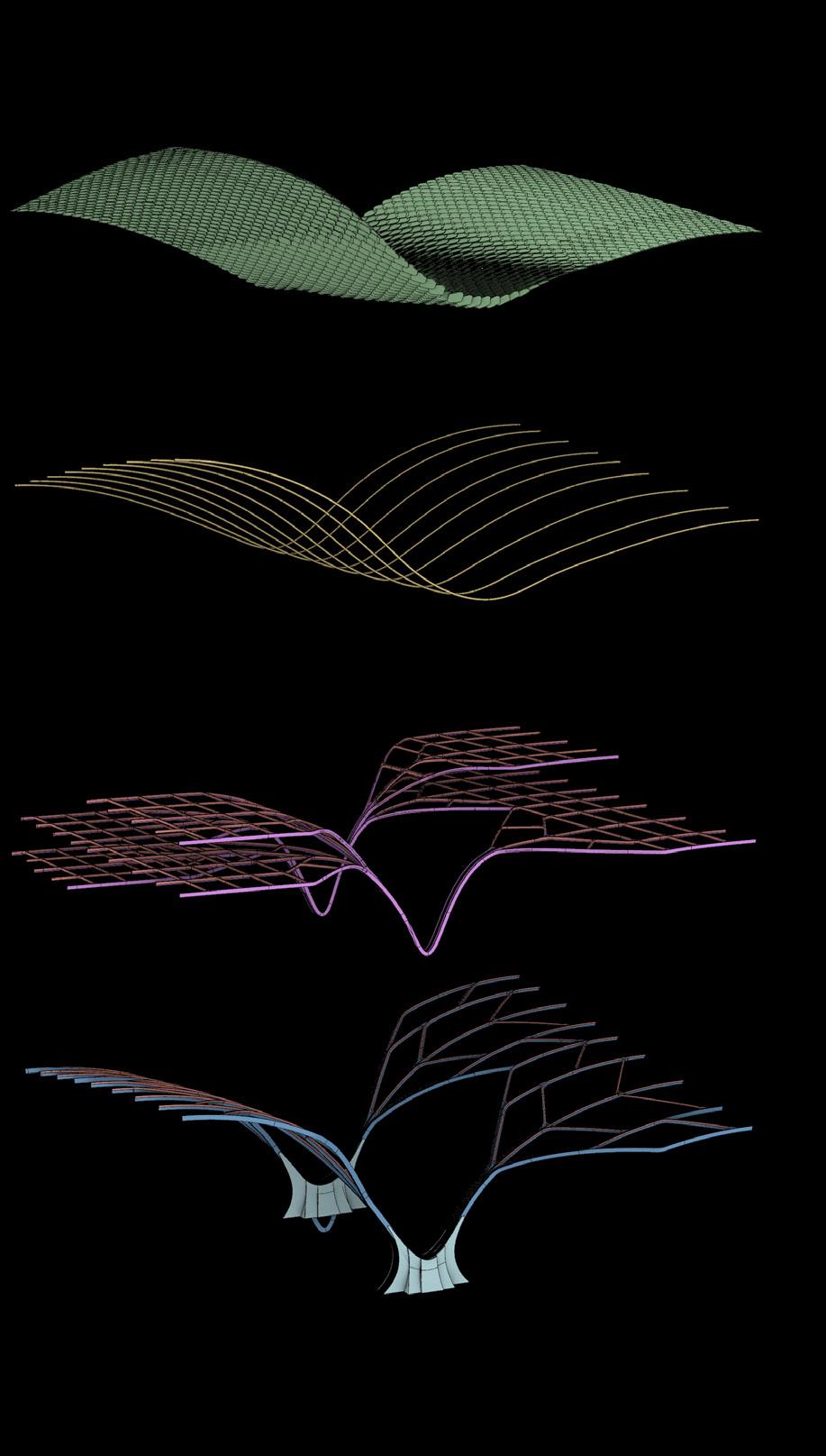
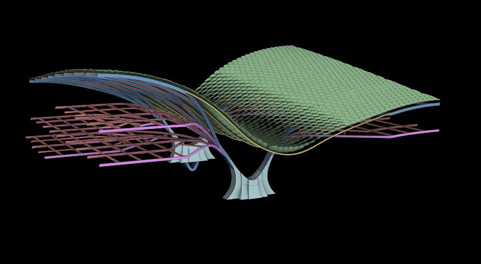
Based on this system, a Grasshopper script is developed that mimics branching in nature within a designated Region (A1). Next, one or multiple Start Points are defined (A2). To start the branching process through “Shortest Walk” path-finding, random Seed Points are generated through 2D Population (A3). However, Seed Points are oriented along the rationalised stress lines and supporting perimeter for the Conoid Shell project, shown in Fig. 2.31. The branches’ Shortest Walk (A5) is specified through Proximity Definition (A4): The fewer the points, the straighter the branch paths will be. Lastly, the Nurbs Curves indicate the smoothness of the overall bifurcation system. Fig. 30 explains the Grasshopper script and the related graphical breakdown of the Lindenmayer-System.

c

F

F →FF-[-F+F+F]+ [+F-F-F]

Figure1.24:Examplesofplant-likestructuresgeneratedbybracketedOLsystems.L-systems(a),(b)and(c)areedge-rewriting,while(d),(e)and (f)arenode-rewriting.

Fig. 2.28 Basic L-System Production Rules and Results After Two and Three Generations (Top) L-Systems have a set of production rules, which are repeated through a few recursions or generations

Fig. 2.29 Plant-Like Structures Generated by Bracketed 0L-Systems (Bottom) L-systems (a), (b) and (c) are edge-rewriting, while (d), (e) and (f) are node-rewriting

the Lindenmayer Branching System (Grasshopper)

L-System mimics biological branching and enables efficient directional deforming (“shortest walk”), which helps to save material

Fig. 2.30 Breakdown of

The

Branching Variations

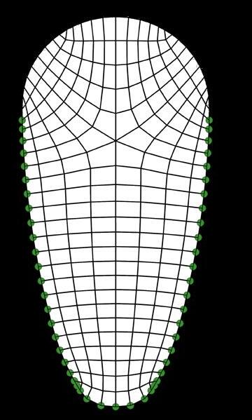
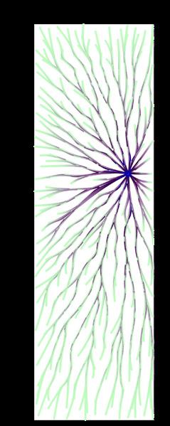
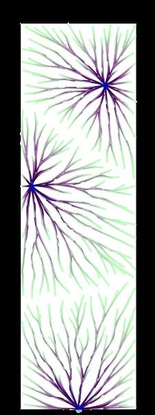
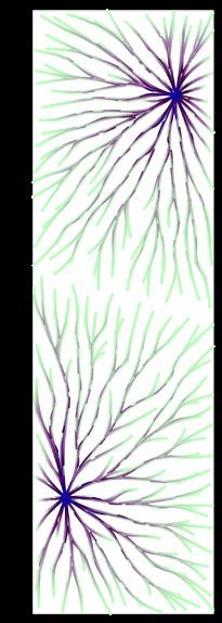
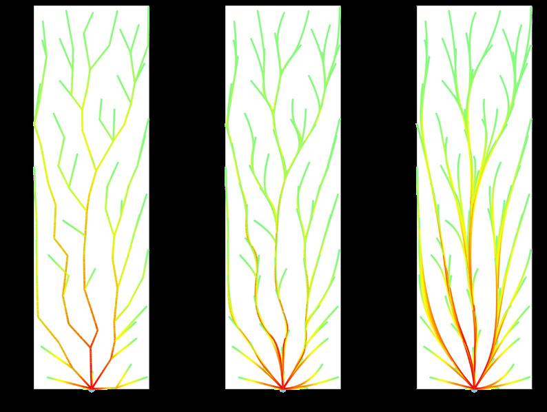
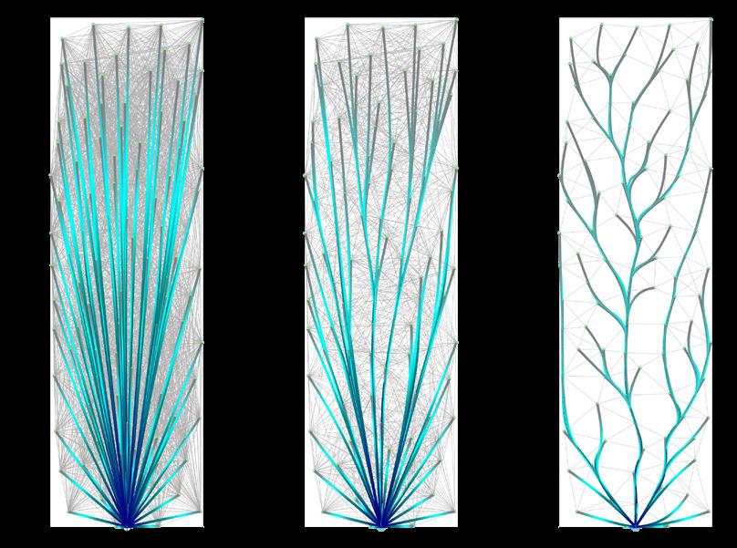
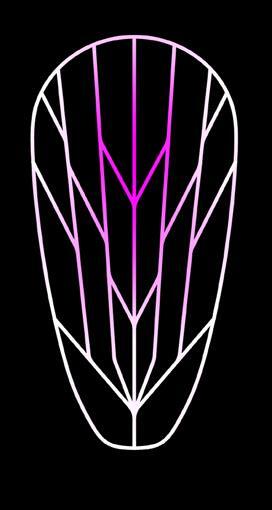
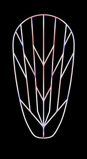
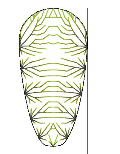
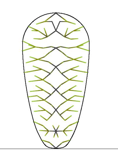
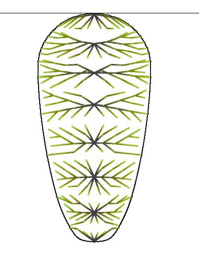
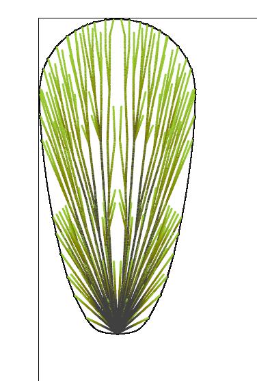
The following three variations will investigate the rationalised L-System bifurcation adapted to the Conoid Shell perimeter and projected onto its surface. Seed Points of all three variations are placed onto the shell’s stress lines, as shown in Fig. 2.25b. Iteration 3a has a single Start Point placed at the end opposite the cantilever (Fig. 2.31a). Iterations 3b and c have multiple Start Points located at the perimeter (Fig. 2.31b) and along the Y-axis vertex (Fig. 2.31c)

Iteration 3a: Single Starting Point

This iteration showcases the L-System bifurcation system with a single starting point at the end opposite the cantilever (Fig. 2.32). Even though the branching follows seed points arranged along the stress lines, the material distribution does not make sense from a structural point of view. As the volume of material is highest at the Start Point, the branches thin out towards the rest of the perimeter, especially at the cantilever, where more material is required. This issue is also reflected in the displacement diagram, where deformation is exceptionally high where axial compression forces are located. To solve this issue, Start Points need to be placed more logical in force flow.

Fig. 2.31a, b, c Branching Variations Using the Lindenmayer-System (3a, 3b, 3c) (Top) Differentiating locations of starting point(s) create different branching pattern outputs

Fig. 2.32 Variation 3a - Rationalised (Bottom) Application of tension members to overhang

Iteration 3a | Start point: Bottom

Iteration 3b | Start points: Perimeter

Iteration 3c | Start points: Y-Axis Vertex

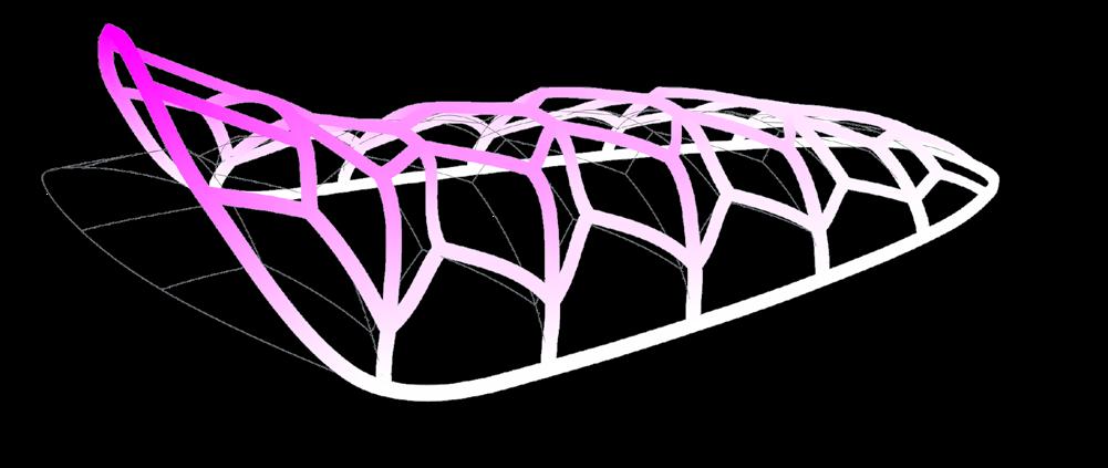
Iteration 3b: Perimeter Starting Points

A system change through relocation of Starting Points can avoid dominant displacements caused by inappropriate material distribution. Therefore, this iteration showcases the L-System bifurcation system with multiple starting points at the perimeter (Fig. 2.33)

Structurally, this branching network works better than iteration 3a, as the support members are the thickest and most dense where the forces flow together. There is minor displacement in the cantilever area that can be addressed through cross-section optimisation (see Section 2.8).

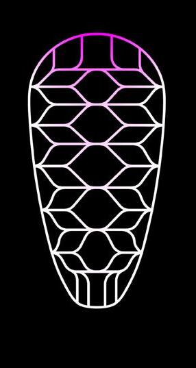
For the most part, gridshells are confined to roof or pavilion structures. Required slab and circulation systems function as separate, independent entities.

However, this branching strategy offers the opportunity to integrate slabs by separating glulam splices near the Starting Points at the perimeter. Using that technique, slab systems can be spatially integrated as part of a continuous structure.

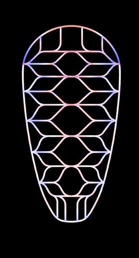
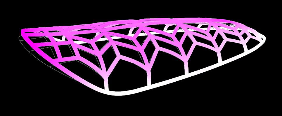
Iteration 3c: Y-Axis Vertex Starting Points

This iteration showcases the L-System bifurcation system with multiple starting points at the Y-axis vertex (Fig. 2.34)

The structural logic of this branching strategy is similar to iteration 3b. Nonetheless, less timber is used while achieving similar displacement output, making this variation more material-efficient. It also responds better to lateral forces as all splices are interconnected.

Due to the horizontal alignment of the branching “trees”, most of the blanks are single-curved. Only the splices shifting away from the x-axis experience slight double curvature. Nevertheless, these diagonal splices help to brace the system.

Analogous to 3b, slabs and circulation can be integrated into the branching network. However, it is essential to mention that the slabs will be non-funicular and be exposed to dead and live loads. For that reason, crosssections need to be adapted accordingly.

Due to the improved properties, further investigations will be conducted using variation 3c.

Application of tension members to overhang

2.8 Cross-Section Optimisation

2.8.1 Main Members

Define Elements (Beams)

Define Cross-Sections --> Depth: 300-600mm

Define Supports

Define Loads --> Meshload Const

Define Material --> Timber

OptimizeCrossSections

Material Distribution (RhinoVAULT 2.0)

To analyse material distribution, a Pipe Diagram is generated in RV2, as demonstrated on the shell structure in Section 2.6. For this simulation, a Pattern is created with the FromLines command in the RV2 drop-down menu. The lines represent an abstracted version of iteration 3c’s branching network. As expected from the displacement and utilisation diagrams, more material is needed around the cantilever. With the widest span of 11.0m, the Conoid Shell’s largest cross-section will have a depth of 450mm, while the smallest cross-section will have a depth of 200mm (Fig. 2.35)

Cross-Section Optimisation (Karamba3D)

Karamba 3D’s Optimize Cross-Section component automatically picks the best cross-sections for beams and shells. It considers the cross-load-bearing section’s capacity and, if desired, restricts the structure’s maximum deflection (Karamba, 2022). The OptiCroSec component calculates each element’s cross-section to ensure that its load-bearing capability is adequate for all load cases (Fig. 2.36). Karamba3D uses the following procedure to do this:

1. Define Elements: Using the abstracted branching network, section forces at nSample points along all lines are determined. The stiffness of the members, i.e. crosssection and materials, influences the section forces in statically indeterminate structures.

2. Define Cross-Sections: The beam depth range is set from 300-600mm so that depth variations lie within the 200-450mm determined via the Pipe Diagram in RV2.

3. Define Supports: The points where the branching line network converges with the perimeter are selected.

4. Define Loads: The type of load is set to MeshLoad Const - the input will be the Conoid Shell surface.

5. Define Material: The defined material is wood. An advantage of using Karamba 3D’s Cross-Section Optimizer alongside RV2’s Pipe Diagram is the possibility of visual demonstration of the varying crosssections of a beam. High curve subdivision allows for the determination of many section forces, leading to a smooth output demonstration.

Fig. 2.35 Material Distribution RhinoVault 2.0

(Top) Differentiating locations of starting point(s) create different branching pattern outputs

Fig. 2.36 Cross-Section Optimisation Karamba3D

(Bottom) Application of tension members to overhang

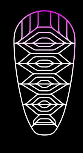
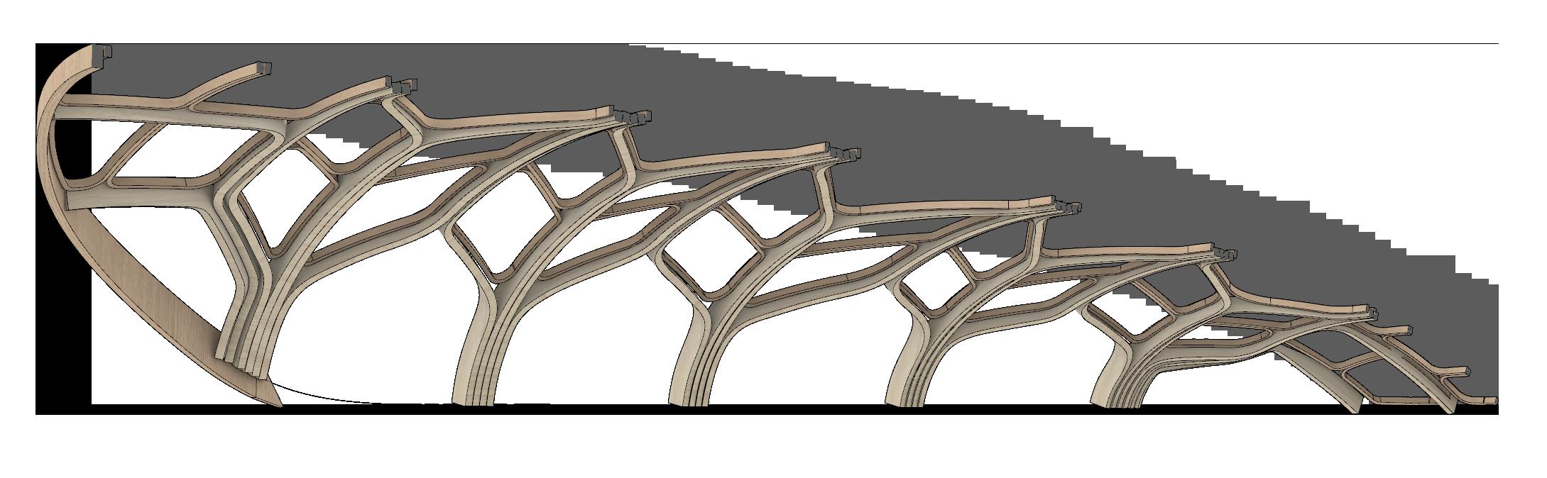
2.8.2 Secondary Members (Lateral Stiffening)

Primary and Secondary Members

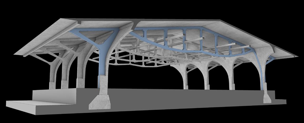
The results from cross-section optimisation are implemented onto the branching system to achieve uniformly distributed loads in the structure (Fig. 2.37). Secondary, lateral stiffening elements can help to further stabilise the structure (Fig. 2.38), as demonstrated in the deformation analysis.

Fig. 2.37 Main Member Material Distribution (Top) Differentiating locations of starting point(s) create different branching pattern outputs

Fig. 2.38 Added Secondary Strcture for Lateral Support (Bottom) Model deflects less in X-direction after the addtion of lateral stiffening

Cantilever: Pollmeier Beech

Lateral Bracing: Pollmeier Beech Spruce: Binderholz Spruce

Fig. 2.40 Bending Magnitude (Top) The secondary structure has the highest bending magnitude, requiring beech LVL for implementation

Fig. 2.41 Wood Species Selection (Middle) Pollmeier beech and Binderholz spruce

Fig. 2.42 Final Timber Roof Structure (Bottom) Rendered axo

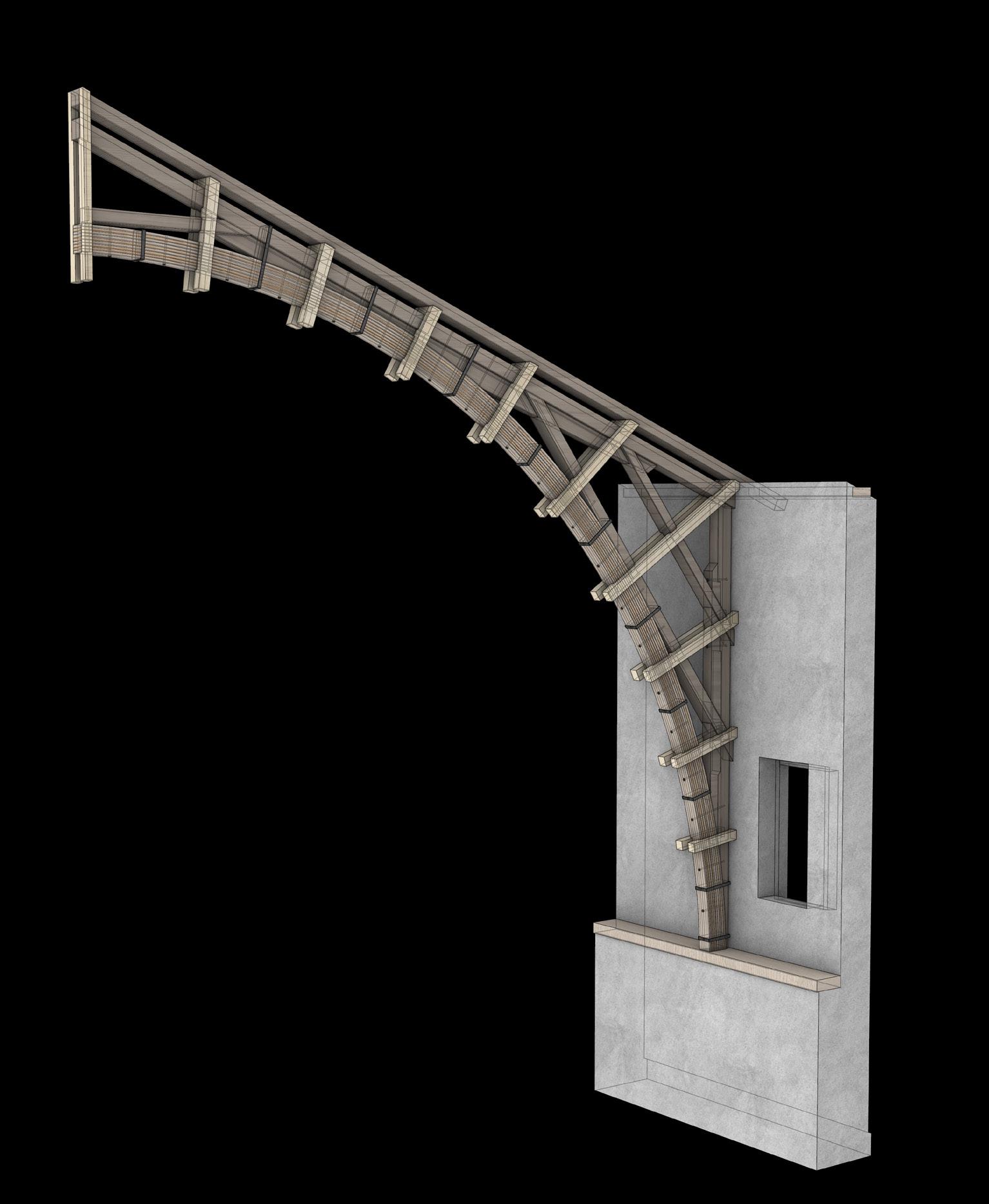
2.11 Ground Connection

Foundation and Structural Wood Protection

An essential aim of the design is to make the structure as longlasting as possible. Structural wood protection is a precaution to increase wood’s lifespan and make the building more ecological. The wood moisture content should be held below 20% to prevent fungal infestation. Timber preservation is given through avoidance of direct ground contact. The foundation height of the project is >30cm, protecting the wood from splash water and contact with damp subsoil (Fig. 2.46). With that, chemical wood preservatives can be omitted. A roof overhang, which protrudes at least 30cm over the wooden structure, also protects the underlying timber (See Section 3)

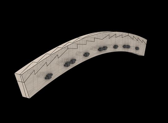
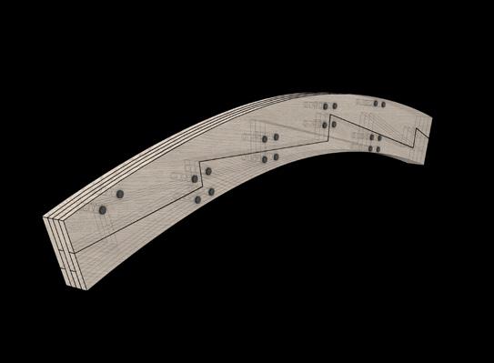
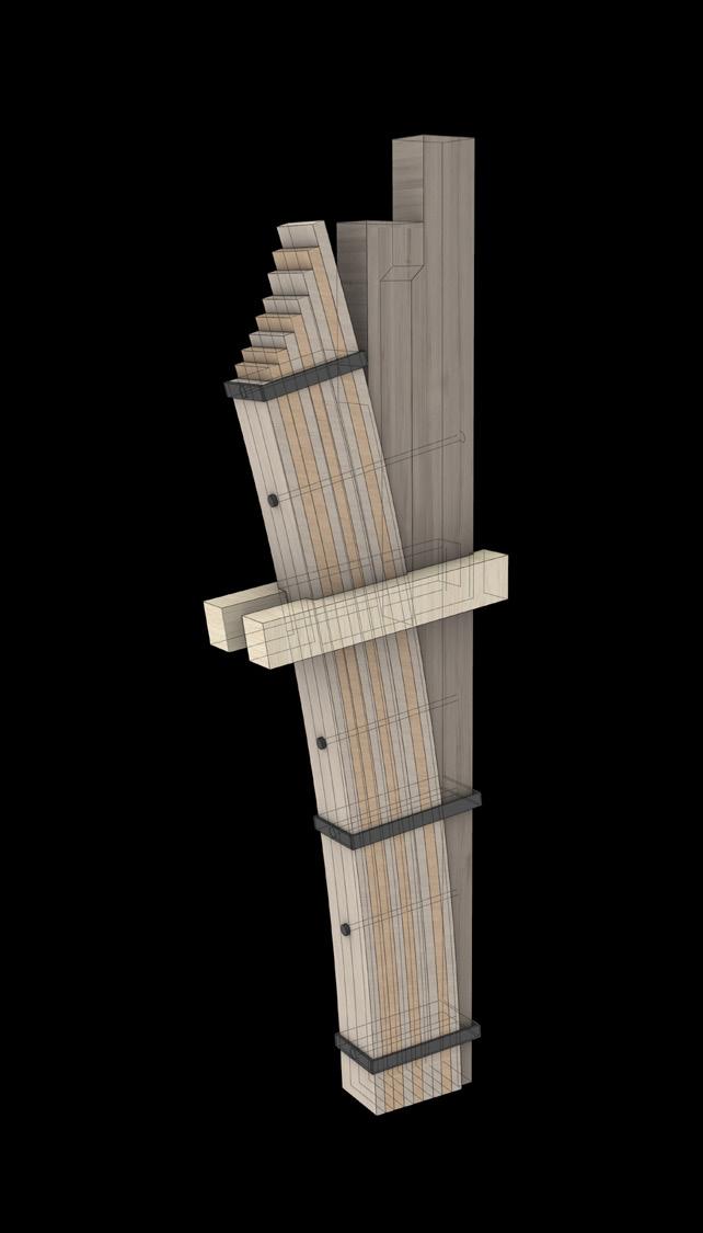
Architecturally, the transition from wood to concrete can also be elegantly accentuated. Based on examples of Japanese timber joinery, a finger tenon joint with notches following the stepped glulam splices can help connect the two materials (Fig. 2.47) The notches offer an almost rigid composite action between timber and concrete and provide continuous load transmission without additional steel fasteners such as screws or dowels (Müller and Frangi, 2021).

Fig. 2.46 Ground Connection Investigation (Top) Foundation serving as wood protection structure (Design Studio Drawing)

Fig. 2.47 Conoid Shell Project Ground Connection (Bottom) Stepped Tenon joint created through stepping of glulam splices

Final Outcome

The use of different timber species takes advantage of the static properties of the distinct species and visually highlights the structural hierarchy. The implemented foundation system helps protect the timber from moisture and contributes to the structure’s longevity (Fig. 2.48, 2.49a, b, c)

This concludes the Conoid shell digital workflow demonstration. Further investigation with the application of the workflow onto more complex shells is illustrated in Section 3

Fire safety

Fire safety needs to be carefully considered with long-span structures like this example. In a fire, timber structures with a broad cross-section remain highly stable. Glulam has a modest penetration rate of 0.5–1 mm per minute (Fig. 2.50). The charcoal layer that accumulates on the surface of the glulam acts as insulation in the first instance and can slow down the rate of burn (Swedish Wood, 2021).

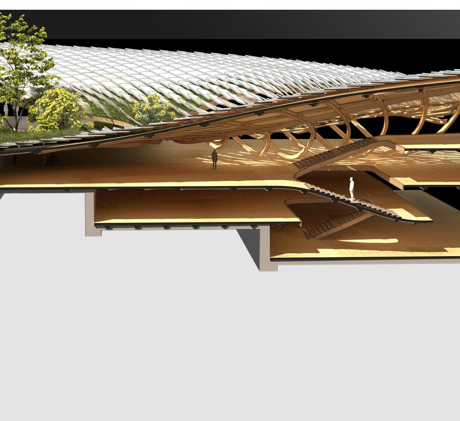
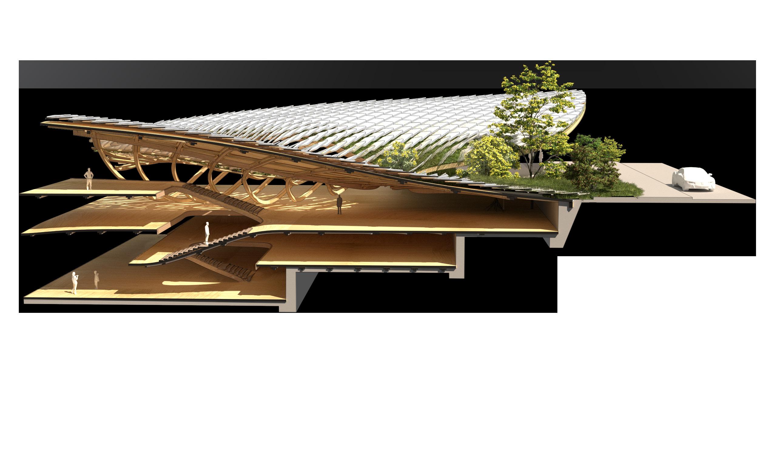
Fig. 2.48 Final Sectional Perspective (Top) Conoid shell branching with integrated slab, circulation and structural timber protection (foundation system)

Fig. 2.49a, b, c Final Elevations (Middle) Side, top, and back view

Fig. 2.50 Glulam Fire Penetration Rate (Bottom Right) Glulam beam after 30 minutes of burning (centre) and after 60 minutes of burning (right) in a four-side fire attack

Top Side

There are three standard methods to reduce the flaring attributes of wood:

1. Construction requiring a fire resistance of 30, 60, and 90mins can be achieved through appropriate dimensioning according to the fire penetration rate.

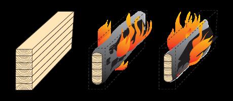
2. Water-borne synthetic chemicals are impregnated into the wood during impregnation treatment. Many synthetic compounds have fire-retarding qualities; however, only a few are regarded as generally feasible due to cost or other considerations.

3. Coatings on wood surfaces are another method for altering the flame characteristics of wood (e.g., intumescent paints). It functions as a thin-film coating that significantly improves fire resistance.

-This page is intentionally left blank-

Studio Project Synthesis

3.2 Project Description

The project site is located on the Theresienwiese in Munich, where the Oktoberfest takes place (Fig. 3.2). It was chosen due to its lack of usage, while the Oktoberfest does not occur. The site is effectively operated for only 53 days a year and is unusable during the temporary infrastructure’s assembly months. Even though there were debates on building onto the site, nothing has been implemented so far, as the festival has sentimental value to the locals.

Therefore, the project idea is to build a permanent structure that facilitates indoor and outdoor spaces for the Oktoberfest while providing a structure for other activities during the off-season, including other festivals and exhibitions. With this measure, value can be added to the deserted space.

In search of the building typology, the Olympic Park, designed by Frei Otto and Günther Behnisch, serves as a role model for creating an urban park as it successfully synthesises the city and landscape (Fig. 3.3). The case study also embodies the Munich sentiment of praising both the established and the innovative.

Timber construction is a traditional and widespread building method in Bavaria and has regained popularity in recent years due to its sustainability - especially in larger-scale projects. The new festival space structure aims to exploit the characteristics of glued-laminated timber to create an advanced structural system through the computational approach presented in Section 2. The project’s footprint provides the perimeter for particle-spring formfinding.

Bavaria Statue and Hall of Fame

Fig. 3.2 Site Plan: Theresienwiese Munich The building footprint serves as the perimeter for shell generation

Munich

Fig. 3.3 Case Study: Olympic Park Munich, Frei Otto, Günther Behnisch, 1972 Creating an urban park: The building as part of the landscape

3.3 Perimeter and Shell Form-Finding

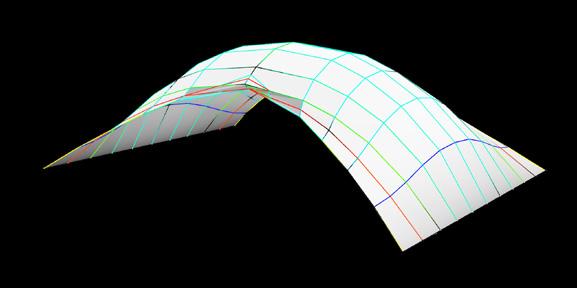
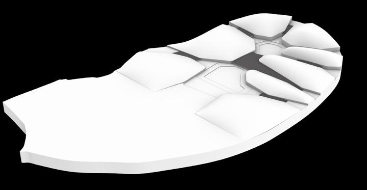
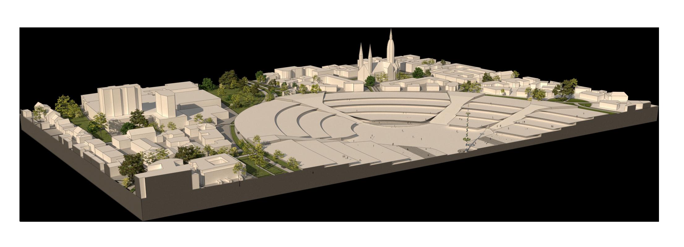
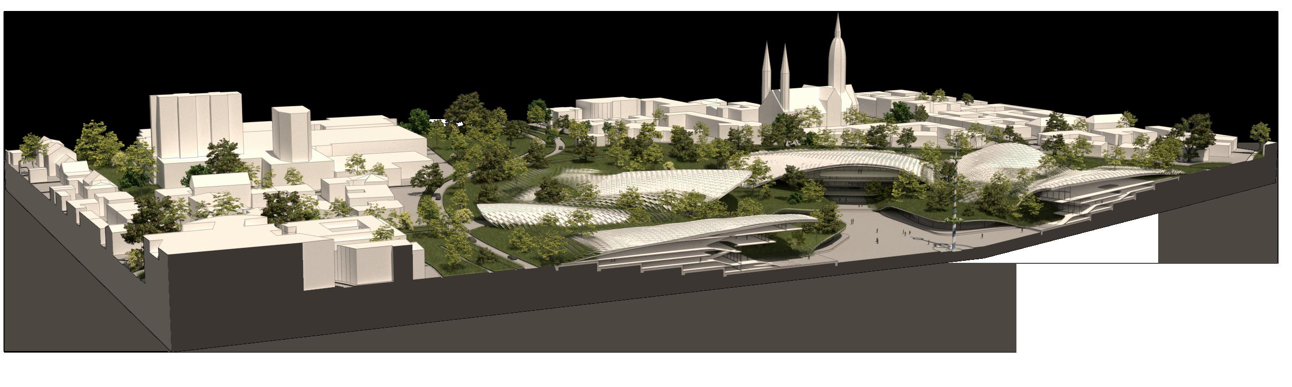
The idea behind the global form is to create a canyon-like condition where the buildings seem carved out of the site. The terrain steps down towards a central plaza. The advantage of this urban strategy is the seamless integration of the landscape and the possibility of creating multi-level stories without severely impacting the existing urban fabric. The sections show that the cascading landscape allows for the terracing of the slabs to evenly distribute direct sunlight on all floors (Fig. 3.5a)

The diagrams in Fig. 3.4 illustrate the global form design genesis. Using the building footprints as perimeters, the funicular roofs are quickly generated with Kangaroo 2 to get a general overview of the roof height and rough shape. Since Kangaroo has no builtin analysis tools, RV2 is used to determine and alter the shell in further design stages.

Before starting analysis, the funicular shape can be modified for aesthetic, programmatic or site-specific purposes. As demonstrated in Section 2.8, these changes can be compensated through cross-section adaption.

Since the Conoid Shell example examined in Section 2 resembles the studio project, the same procedure is used to create and analyse openings and overhangs. Free boundaries are created to avoid edge relaxation in these areas. Therefore, the cantilever edges of the Force Diagram are flipped from compression to tension with the FlipEdge command in the ModifyForceDiagram settings.

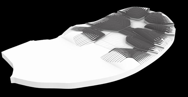
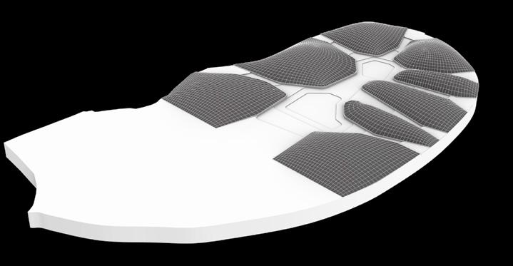
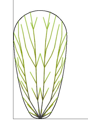
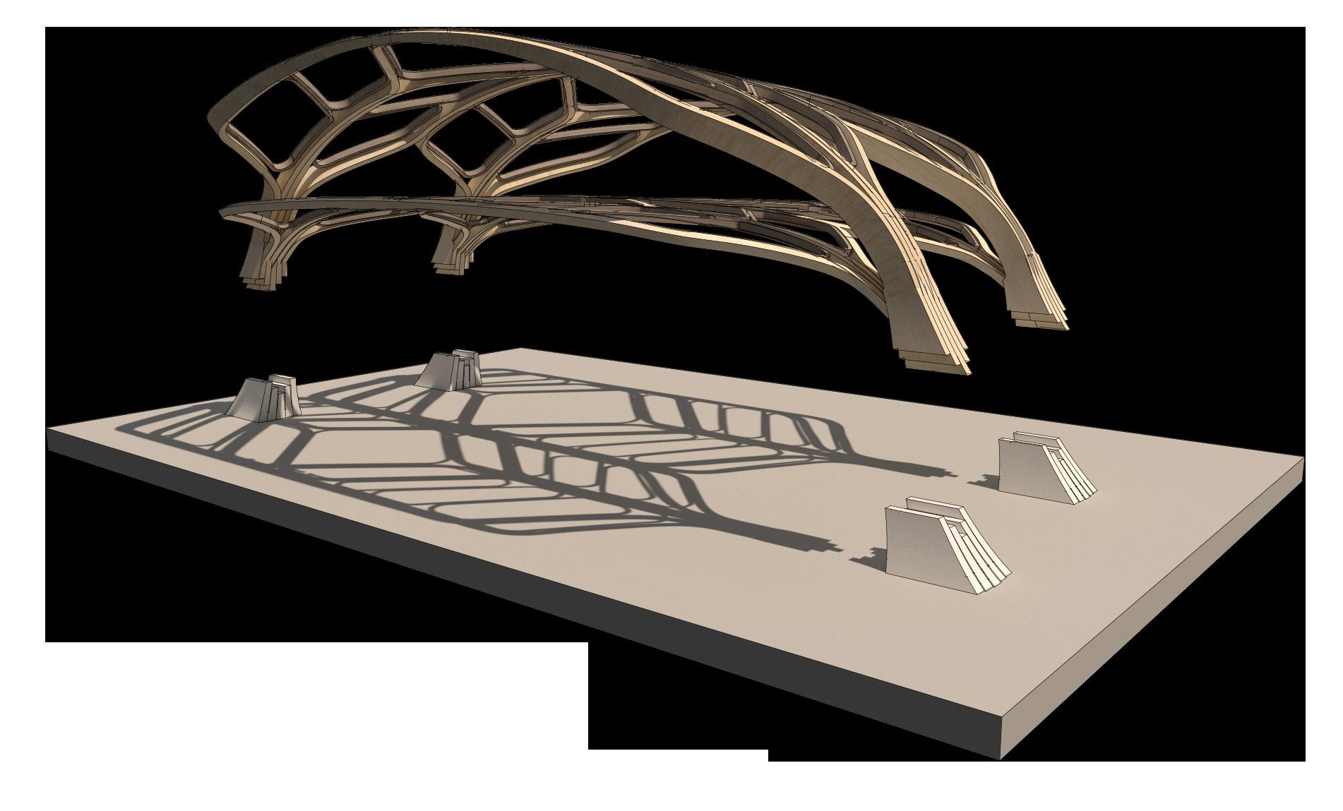
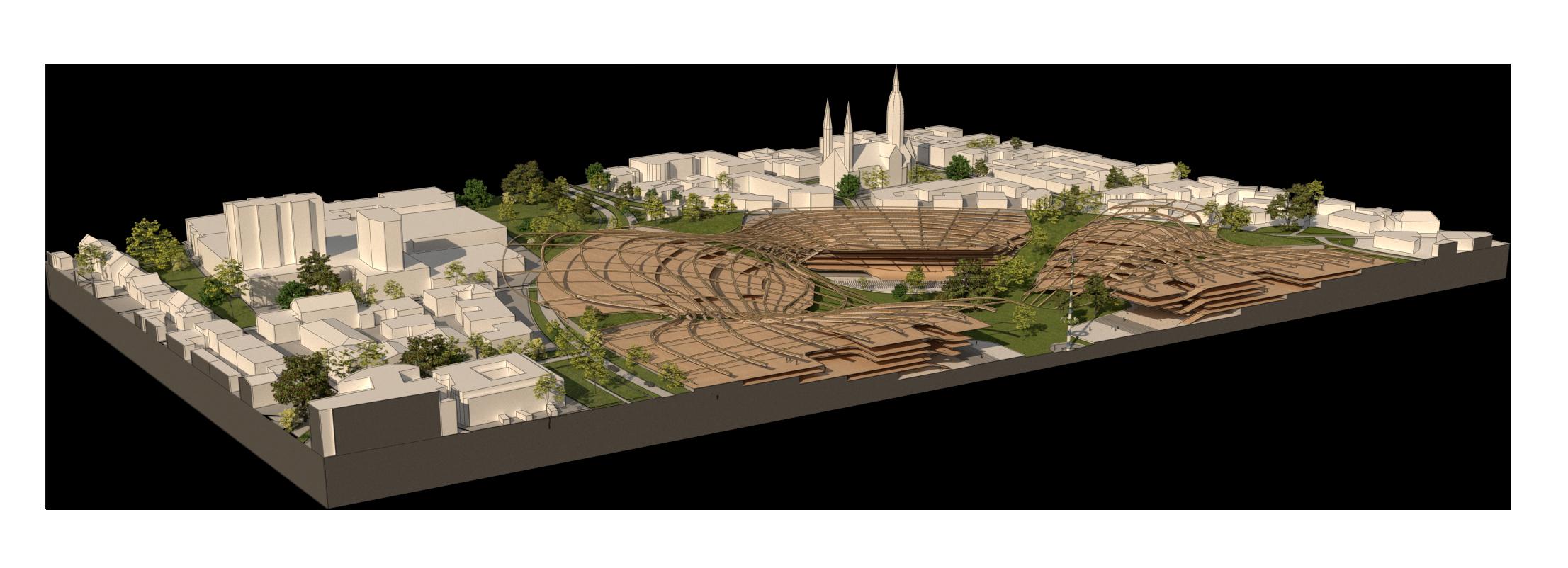
After force analysis, the branching system is generated using the L-System script with Seed Points placed onto the shell’s stress lines. The output is then rationalised (Fig. 3.5b), and doublecurved elements are avoided as much as possible. Non-funicular elements such as slabs and circulation are integrated into the structure.

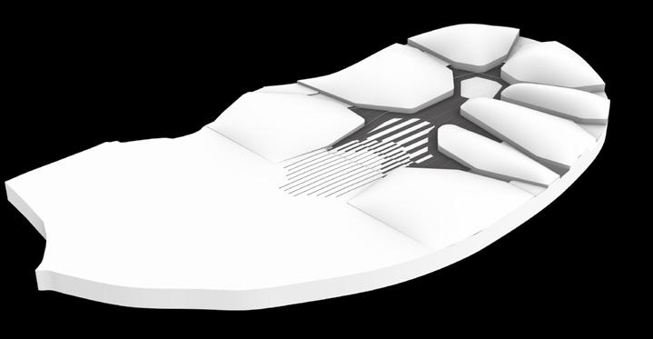
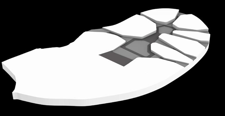
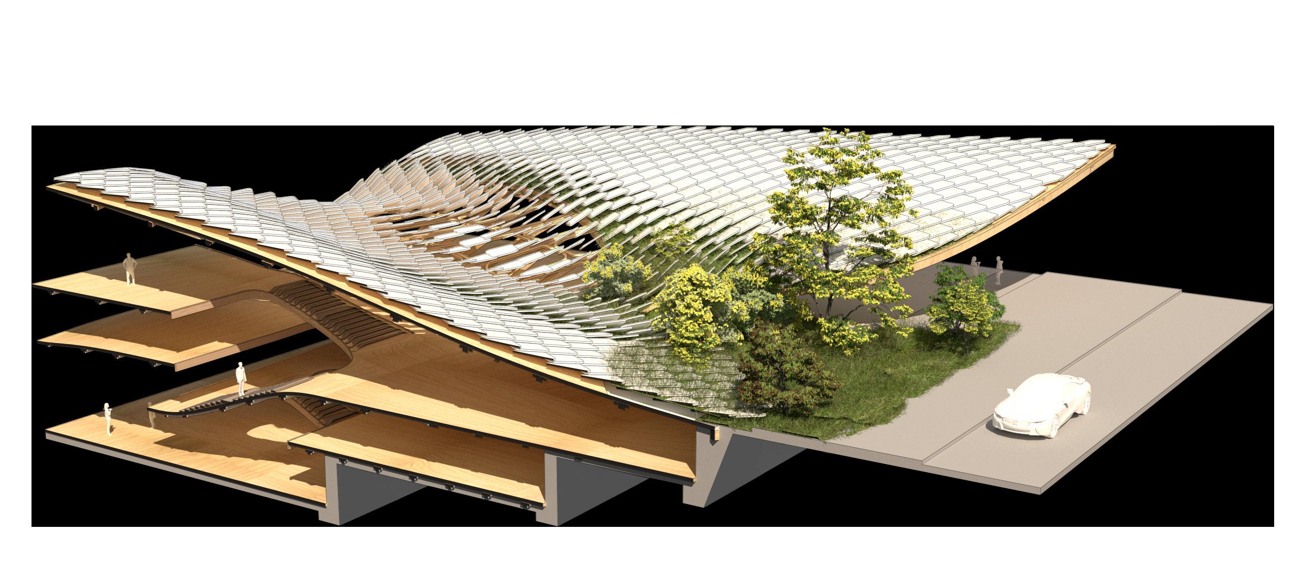
Finally, a clay shingle roof is implemented to protect the timber structure and impose a sense of scale. The tiling system formalises the large surface areas and allows for greenery to grow in defined areas so that the structure can become part of the landscape (Fig. 3.5c)

3

5 Greenery Transition - Ground

Roof generation (Kangaroo 2, RhinoVault 2.0)

6 Greenery Transition - Buildings

Fig. 3.4 Global Shape Funicular roof generated through RhinoVault 2.0 and Kangaroo

Fig. 3.5 Full Site Sections

Ground terracing, RV2 analysis and glulam structure, roof tiling and landscape integration

3.4 Branching Application

Similar to the demonstration in Section 2.6, the Utilisation analysis in Karamba shows that the structure experiences compression around the shell’s vertex and the cantilever edges and tension around the supported perimeter, especially in the segments connecting the buildings.

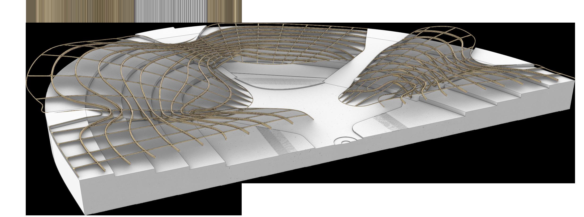
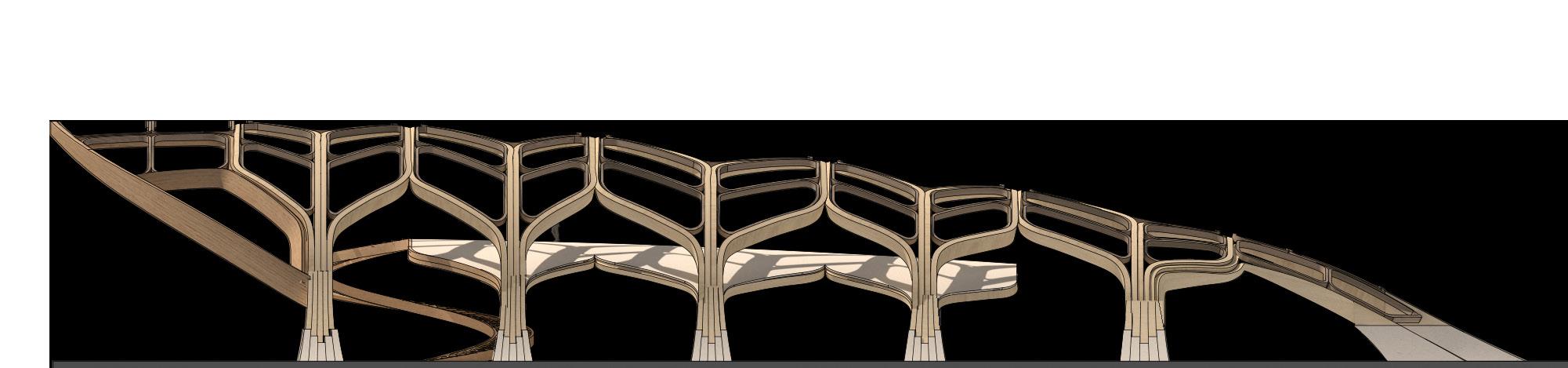
Fig. 3.6 depicts the Karamba shell analysis and the rough structural outline responding to it. Cross-sections have more depth in the overhangs and connecting areas around the perimeter. The glulam beams gradually get more slender towards the shell’s vertex as forces decrease.

Fig. 3.7 illustrates the structural branching system in a more detailed fragment (with consideration of lateral bracing). Slab beams are thicker as they are non-funicular and exposed to live loads. The foundation is a tenon joint with notches following the stepped glulam splices, allowing continuous load transmission. Foundation concrete height is kept at >30cm for structural wood protection. Overhangs and clay roof tiles also protect the timber substructure.

Fig. 3.6 Branching System Using the L-System (Simplified) Karamba Analysis (Principle Stress and Stress Lines)

Tiling

Roof Substructure

Integrated Slab System (non-funicular)

Roof/Enclosure System

Assembled Model

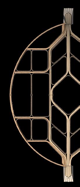
Fig. 3.7 Branching System Using the L-System (Detailed) Structural build-up of a fragment

Opened tiles

Tiling

1 Heat-reflecting clay tiles (white) 50mm

2 Substructure tiling system

3 Steel fixing rod Ø 20mm

Intensive green roof Vegetation

4 Growing substrate 200mm

5 Filter layer5mm

6 Drainage layer 60mm

7 Root barrier 5mm

8 Protection mat 10mm

9 PVC waterproof membrane 1mm

10 Expanded Polystyrene insulation (EPS) 140mm

11 Vapour control layer 1mm

12 Timber cladding 20mm

Closed tiles

Roof structure

13 Pollmeier® Baubuche GL75 beech LVL beam (secondary) 200x60mm

14 Spruce glulam beam (primary) 600x120mm

Skylight

15 Triple-glazed laminated glass (LG) 10mm

16 Aluminium window frame

Roof Structure (no vegetation)

17 Timber battens 20mm

18 Pollmeier® Baubuche GL75 beech LVL beam (secondary) 200x60mm

19 Spruce glulam beam (primary) 400x120mm

Fig. 3.8 Roof Structure Detail

(Top) Intensive green roof allows the building to become part of the landscape

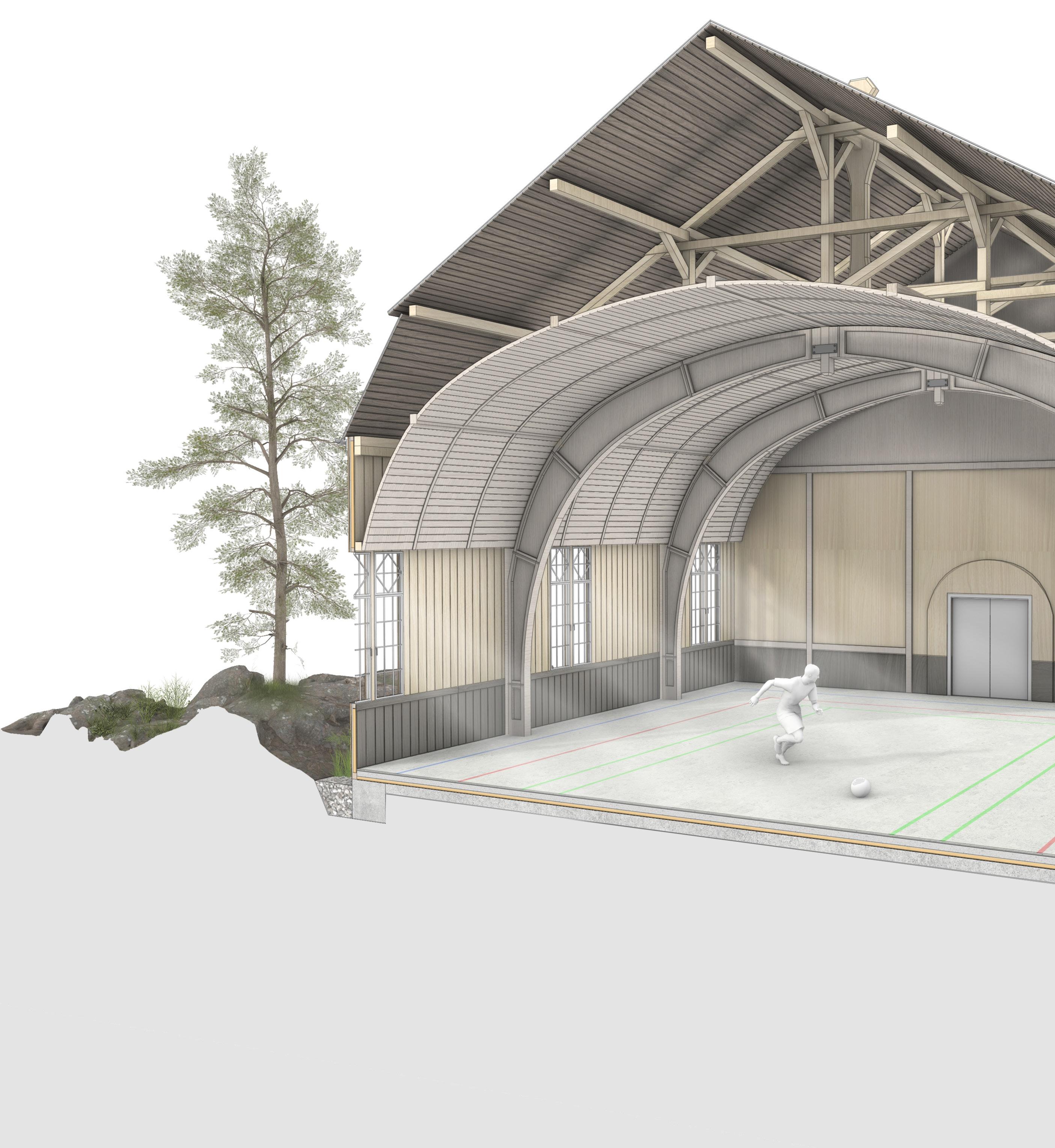
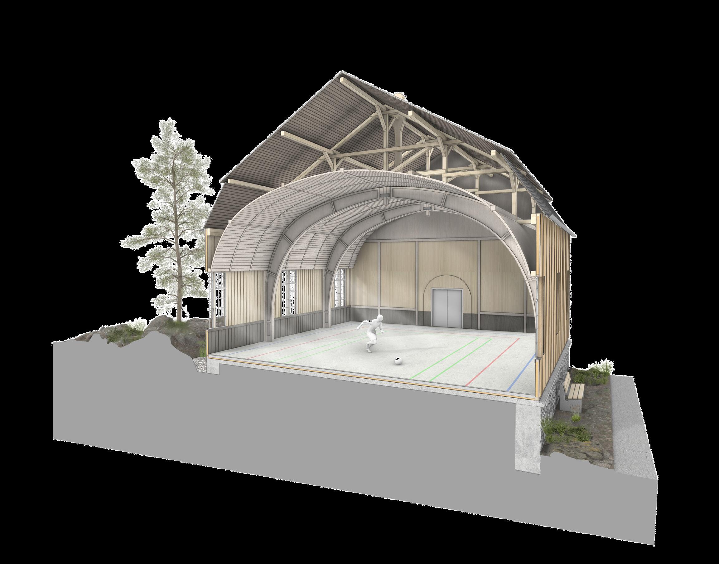
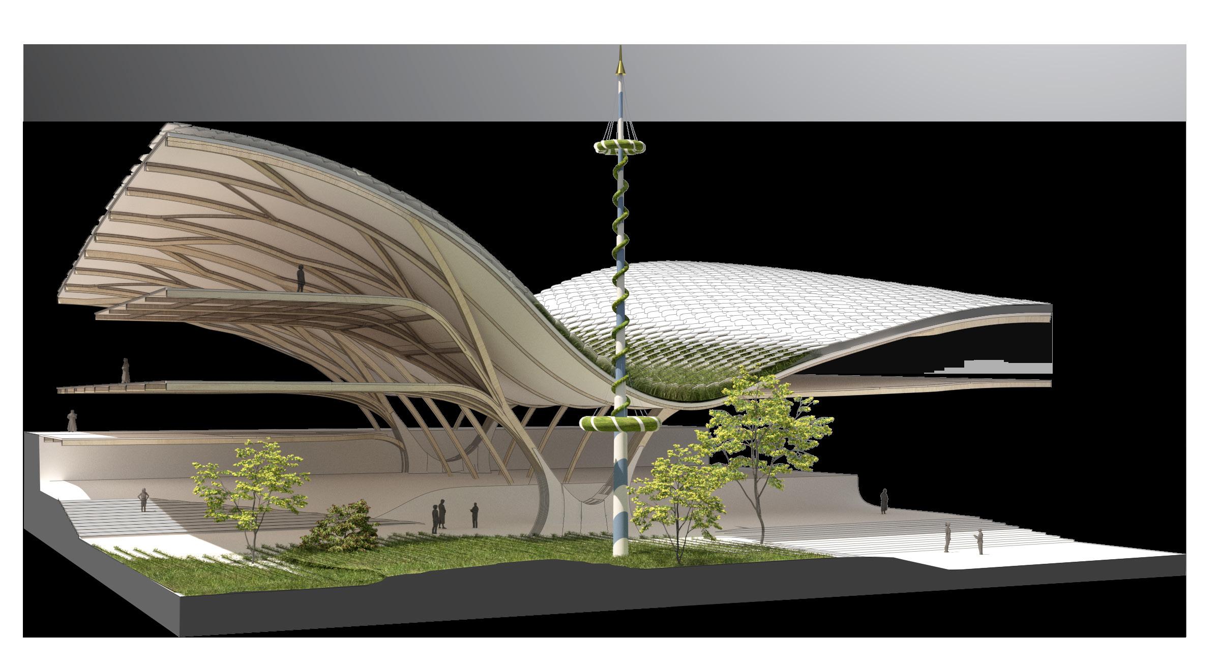
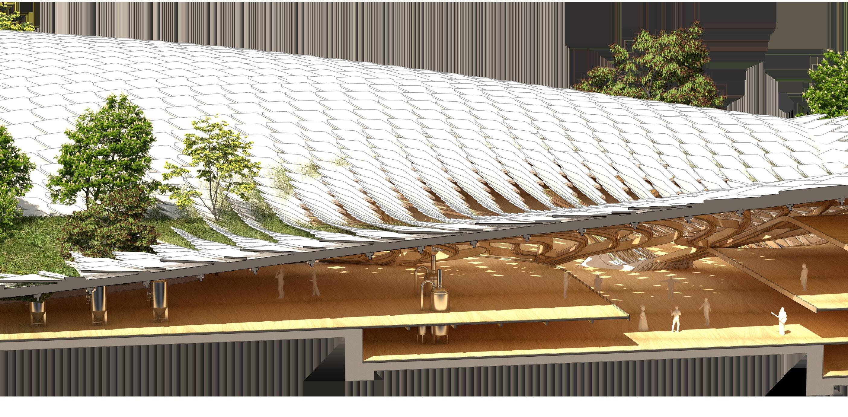
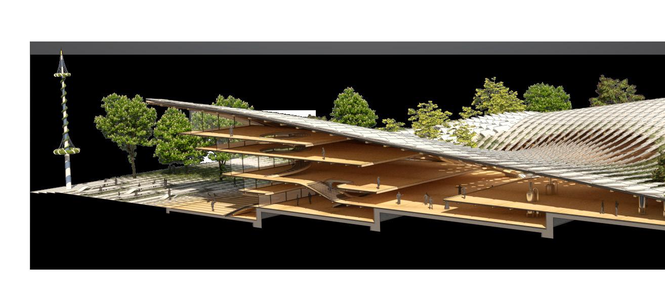
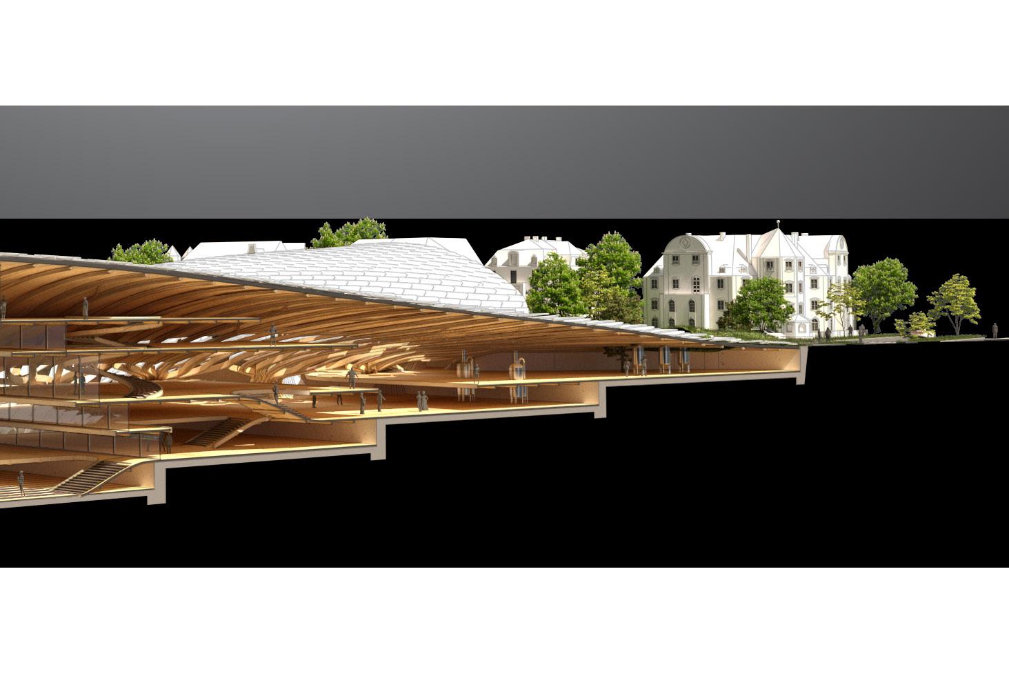
Fig. 3.9 Sectional Perspective

(Bottom) Interior lighting is established through rotated shingle openings

3.6 Final Views

The next series of building fragments show the project’s relation to the street, surrounding buildings, and the green plaza. Timber and slate shingles are very popular in Bavaria; therefore, the project possesses a contemporary heat-reflecting clay tile covering. The parametric rotation system opens wherever the envelope touches the ground to let the grass grow between the tiles. Daylight comes in through the openings in the centre of the roof.

Fig. 3.10 Relationship Interior-Exterior Greenery grows on the roof where it dips down; the wood paneling in the interior radiates warmth

-This page is intentionally left blank-

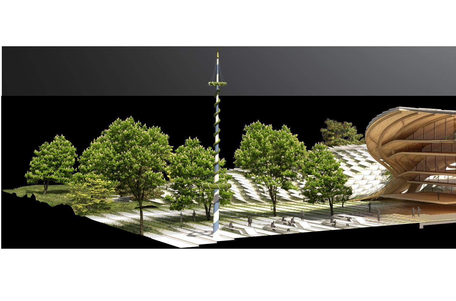
Fig. 3.11 Plaza Relationship

(Top) The plaza works similar to a Volksgarten (people’s garden), where people enjoy the perks of an urban park (e.g., outside dining, Biergarten)

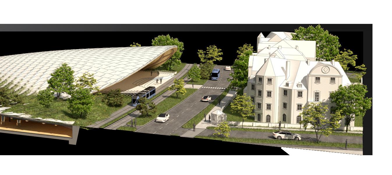
Fig. 3.12 Street Relationship

(Bottom) The building also reacts to the surrounding streets and Gründerzeit building context

Thesis Conclusion

The core of the thesis consisted of establishing a digital workflow in projecting bifurcation systems onto funicular shells while simultaneously allowing architectural exploration. Next to the primary research done through computational experimentation, it was beneficial to gather knowledge about glulam structures through case study examination and literature review.

In the start, it was advantageous to investigate the characteristics and capabilities of timber, the importance of grain direction and the subtle variations of different timber species, which helped to exploit the strengths of the material in design.

Different computational tools helped modify and adapt funicular shapes to accommodate specific site conditions and user needs. Thanks to the link to parametric systems such as Grasshopper, this was made possible. Nonetheless, the investigation showed that the programmes cannot substitute the design process and should be used as analysis tools only.

An advantage of the final branching system selected in Section 2 was the possibility of slab and circulation integration, the provision of lateral bracing and the opportunity for effective material distribution through glulam splice separation. The outcome is a structure with outstanding properties linked to the material, including performance consistency, longevity and fire resistance. As demonstrated in Section 3, this system can also be applied to other shell structures. Different timber species and cross-sections adapted to the analysis make the design structural and materialefficient and establish an aesthetic hierarchy.

However, production costs due to mass-customisation procedures and high prices should not be underestimated. Even though double-curvature is minimised as much as possible, it is not entirely unavoidable, primarily when diagonal branches orient away from the x- or y-axis. Therefore, these elements will always be slightly curved in two directions - and as mentioned in Section 1, producing double-curved glulam blanks is time-consuming and expensive.

Glulam is also made by glueing numerous splices together and then finger-jointing them to other components. When substandard wood is used in the manufacturing of a timber block, the entire block can deteriorate.

The thesis research has shown that industrial timber can achieve amazing things, especially with the support of digital form-finding and analysis tools. As these are in constant development, it is exciting to see what else can be accomplished in the future.

Books

Adriaenssens, S. et al. (2014). Shell Structures for Architecture: Form Finding and Optimization. London: Routledge.

Billington, D. P. (1997). Robert Maillert. Builder, Designer, and Artist. Cambridge: Cambridge University Press.

Jeska, S., Pascha K. S. (2014). Emergent Timber Technologies: Materials, Structures, Engineering, Projects. Edited by: Rainer Hascher. Basel/Berlin/ Boston: Birkhäuser.

Menges, A. (2017). Advancing wood architecture: a computational approach. Edited by: Tobias Schwinn and Oliver David Krieg. London: Routledge

Müller, C. (2000). Laminated Timber Construction. Basel/Berlin/Boston: Birkhäuser.

Lennartz, M. W., Jacob-Freitag, S. (2015). New Architecture in Wood. Basel: Birkhäuser.

Published Thesis

Kam-Ming, M. T. (2015). Principal stress line computation for discrete topology design. Master of Engineering Thesis. Massachusetts Institute of Technology. Available at: https://dspace.mit.edu/handle/1721.1/99630 (Accessed: 04 April 2022).

Rippmann, M. (2016). Funicular Shell Design. PhD Thesis. ETH Zurich. Available at: https://block.arch.ethz.ch/brg/files/Final_PhD_ rippmann-2_1468394847.pdf (Accessed: 03 March 2022).

Robinson, M. (2019). File-to-Factory: Transferring design intent to manufacture. M. Arch. (Professional) Thesis. Victoria University of Wellington. Available at: https://openaccess.wgtn.ac.nz/articles/thesis/ File-to-Factory_Transferring_Design_Intent_to_Manufacture/17148746

(Accessed: 26 February 2022).

Svilans, T. (2021). Integrated material practice in free-form timber structures. PhD Thesis. The Royal Danish Academy of Fine Arts, Schools of Architecture, Design and Conversation. Available at: https://discovery. ucl.ac.uk/id/eprint/10121947/1/Svilans%20-%202020%20-%20 Integrated%20material%20practice%20in%20free-form%20timber%20 structures.pdf (Accessed: 13 February 2022).

Toussant, M. H. (2007). A Design Tool for Timber Gridshells. MSc Thesis. TU Delft. Available at: https://homepage.tudelft.nl/p3r3s/MSc_projects/ reportToussaint.pdf (Accessed: 13 February 2022).

Book Chapters

Green, D. W. (2001). ‘Wood: Strength and Stiffness’ in Bushow, K. H. J., Flemings, M. C., Kramer, E. J., Veyssière, P., Cahn, R. W., Ilschner, B. and Mahajan, S. (eds.) Encyclopedia of Materials: Science and Technology. Amsterdam/New York: Elsevier, pp. 9732-9736.

Harte, A. (2009). ‘Timber engineering: an introduction’ in Forde, M. (ed.) ICE manual Construction Materials: Volume I/II: Fundamentals and Theory; Concrete; Asphalts inroad construction; Masonry. Institution of Civil Engineers, pp. 707-715.

Self, M. and Vercruysse, E. (2017). ‘Infinite Variations, Radical Strategies’, in Menges, A. et al. (ed.) Fabricate. London: UCL Press, pp. 30-35.

Prusinkiewicz, P. and Lindenmayer, A. (1990). ‘Graphical modeling using L-systems’, in Prusinkiewicz, P. and Lindenmayer, A. (eds.) The Algorithmic Beauty of Plants. New York: Springer, pp. 1-50.

Websites

Baerwald Research (2021). No-nails structural wood – Shigeru Ban’s Tamedia office building. Available at: http://www.baerwaldresearch. com/no-nails-structural-wood-shigeru-bans-tamedia-office-building/ (Accessed: 06 March 2022).

BAM Construct UK (2022). German Gymnasium, London. Available at: https://www.bam.co.uk/how-we-do-it/case-study/german-gymnasiumlondon (Accessed: 09. April 2022).

Binderholz (2022). Produkte. Available at: https://www.binderholz.com/ produkte/brettschichtholz/ (Accessed: 14. April 2022).

Block Research Group (2022). Workflow+UI, Tutorial. Available at: https:// blockresearchgroup.gitbook.io/rv2/quick-start/workflow (Accessed: 04 April 2022).

Buckland Timber (2021). Glulam Timber Species. Available at: https://www.bucklandtimber.co.uk/timber-species/#:~:text=The%20 sapwood%20has%20a%20thickness,density%20and%20good%20 strength%20properties (Accessed: 28 Feburary 2022).

Clearloop (2021). Gate vs Grave: What’s the Best Way to Measure Your Carbon Footprint? Available at: https://clearloop.us/2021/03/24/cradleto-gate-vs-cradle-to-grave/#:~:text=Cradle%2Dto%2Dgate%20refers%20 to,composted%2C%20avoiding%20the%20landfill%20altogether (Accessed 15 April 2022).

Debney, P. (2015). Why It’s Good to be a Lightweight. Available at: https:// www.structuremag.org/?p=8043 (Accessed 24 April 2022).

Engler, N. (2007). The Way Wood Works. Available at: https://www. popularwoodworking.com/article/the_way_wood_works/ (Accessed: 13 February 2022).

HDP Construction (2021). Disadvantage of Glulam Timber. Available at: https://www.hpdconsult.com/what-is-glulam-beam/ (Accessed: 24. April 2022).

Koru Architects (2022). 3 reasons sustainable timber is the best construction material. Available at: https://www.koruarchitects.co.uk/ choose-sustainable-timber/#:~:text=Sustainable%20timber%20has%20 (Accessedthe%20lowest,processing%20compared%20to%20other%20 materials (Accessed: 15 April 2022).

Ochoa, G. (1998). An Introduction to Lindenmayer Systems. Available at: http://www1.biologie.uni-hamburg.de/b-online/e28_3/lsys.html (Accessed: 09 April 2022).

PEFC (2022). Standards and Guides. Available at: https://pefc.org/ standards-implementation/standards-and-guides#:~:text=PEFC%20 chain%20of%20custody%20establishes,health%2C%20safety%20 and%20labour%20issues (Accessed: 15 April 2022).

Pfeiffer (2022). Brettschichtholz. Available at: https://www.pfeifergroup. com/de/produkte/holzbau/brettschichtholz/das-produkt/ (Accessed 15 April 2022).

Pollmeier (2022). Über Baubuche. Available at: https://www.pollmeier. com/de/produkte/ueber-baubuche#gref (Accessed: 05 March 2022).

Karamba3D (2022). Parametric Engineering. Available at: https://www. karamba3d.com/ (Accessed: 04 April 2022).

Knippershelbig (2013). Wilhelma Elephant World. Available at: https:// www.knippershelbig.com/en/projects/wilhelma-elephant-world (Accessed: 05 March 2022).

Spring, M. (2006). Bespoke Savill style. Available at: https://www.building. co.uk/buildings/bespoke-savill-style/3069742.article (Accessed 09. April 2022).

Swedish Wood (2022). Manufacturers & manufacture. Available at: https://www.swedishwood.com/building-with-wood/about-glulam/ manufacturers-manufacture/ (Accessed 14. April 2022).

Swedish Wood (2022). Technical Properties. Available at: https://www. swedishwood.com/building-with-wood/about-glulam/choosing_glulam/ technical_properties/ (Accessed 15. April 2022).

Timber Online (2022). The biggest glulam producers. Available at: https:// www.timber-online.net/blog/biggest-glulam-producers.html (Accessed 14. April 2022).

Trada (2022). Bishop Edward King Chapel, Cuddesdon, Oxfordshire. Available at: https://www.trada.co.uk/case-studies/bishop-edward-kingchapel-cuddesdon-oxfordshire/ (Accessed 24. April 2022).

Wood Awards (2017). Savill Building. Available at: https://woodawards. com/portfolio/savill-building/ (Accessed: 09 April 2022).

Articles

Bergqvist, S. (2020). ‘240 metres of precision’, Wood Magazine, (Summer issue), pp. 14-17.

Scott, R. (2014). ‘Timber Case Study: Bishop Edward King Chapel’, In Touch with Timber, (March), pp. 22-29.

Conference Papers

A. Kalama, D. Tzoni, and I. Symeonidou (2020). ‘Kerf Bending: A Generalogy of Cutting Patterns for Single and Double Curvature.’ 7th International Conference on Geometry and Graphics. Faculty of Mechanical Engineering Belgrade, 18-21 Septenber. Thessaly: University of Thessaly, pp. 1-16.

Harris, R. and Roynon, J. (2008). ‘The Savill Garden Gridshell design and construction.’ 10th World Conference of Timber Engineering. Miyazaki, Japan, 02-05 June. Bath: University of Bath, pp. 1-3.

Kilian, A. (2004). ‘Linking Hanging Chain Models to Fabrication’. Proceedings of the 23rd Annual Conference of the ACADIA. Waterloo/ Buffalo/Nottingham. 8-14 November, pp. 1-17.

Pellis, D. and Pottman, H. (2020). ‘Geometry and Statics of Optimal Freeform Gridshells’. 14. Fachtagung Baustatik – Baupraxis. University of Stuttgart. 23-24 March 2020, pp. 1-8.

Rippmann M. and Block P. (2013) ‘Funicular Shell Design Exploration’. Proceedings of the 33rd Annual Conference of the ACADIA. Waterloo/ Buffalo/Nottingham. 24-26 October, pp. 1-19.

Journals

Kilian, A. and Ochsendorf, J. (2005). ‘Particle-Spring Systems For Structural Form Finding’, Journal of the International Association for Shell and Spatial Structures, 46(147), pp. 77-84.

Larsen, K. E. and Schindler, C. (2008). ‘From Concept to Reality: Digital Systems in Architectural Design and Fabrication’, International Journal of Architectural Computing, 4(6), pp. 397-413. doi: 10.1260/147807708787523312.

Müller, K. and Frangi, A. (2021). ‘Micro-notches as a novel connection system for timberconcrete composite slabs’, Engineering Structures, 245, pp. 1-10. doi: 10.3929/ethz-b-000474874.

Olsson, A., Briggert, A. and Oscarsson, J. (2019). ‘Increased yield of finger jointed structural timber by accounting for grain orientation utilizing the tracheid effect’, European Journal of Wood and Wood Products. 77, pp. 1063–1077. doi: 10.1007/s00107-019-01465-0.

Rippmann M., Lachauer L. and Block P. (2012). ‘RhinoVAULT - Interactive Vault Design’, International Journal of Space Structures, 27(4), pp. 219230. doi: 10.1260/0266-3511.27.4.219.

List of Figures

1. Glulam: History and Development

Fig. 1 Title Page

a, b Drawing by author, design studio drawing

Fig. 1.0 Glulam Spiral Staircase

Drawing by author, design studio drawing

Fig. 1.1 Section 1 Title Page

Drawing by author

Fig. 1.2 “Why timber bends, breaks and remains stiff, and how it can be made rigid”, 1726 Müller, 2000, p.8

Fig. 1.3 Composite beam in Amsterdam City Hall 1648-1645 Müller, 2000, p. 9

Fig. 1.4 De L’Orme System

Drawing by author

Fig. 1.5 Composite Beam Evolution https://www.archweb.com/en/design/page/Laminated-wood/ (11.04.2022), redrawn by author

Fig. 1.6 De L’Orme System Detail

Drawing by author

Fig. 1.7 Hetzer Patent 125895: Load-Optimised Composite Beam Müller, 2000, p. 23

Fig. 1.8 Hetzer Patent 197773: Glued-laminated Timber Beam Müller, 2000, p. 25

Fig. 1.9 Hetzer Patent 125895: Composite I-Beam

Drawing by author

Fig. 1.10 Hetzer Patent 163144: Parabolic Composite Beam

Drawing by author

Fig. 1.11 Case Study: Doecker Gymnasium Wuppertal 1911

Drawing by author

Fig. 1.12 Savill Building Workflow: Digital Perimetre Definition Harris and Roynon, 2008, p.3, redrawn by author

Fig. 1.13 Form-Finding and Analysis Model Harris and Roynon, 2008, p.3

Fig. 1.14 Structural Analysis of the Savill Building Elastic Gridshell Harris and Roynon, 2008, p.4

Fig. 1.15 Case Study: Savill Building Surrey, Glenn Howells Architects, 2006

Adriaenssens, S. et al., 2014, p. 88

Fig. 1.16 The Three Primary Axes of Wood Green, 2021, p. 9732, redrawn by author

Fig. 1.17 Timber Cuts

Drawing by author

Fig. 1.18 Distortion of wood due to shrinkage and swelling Svilans, 2021, p.75, redrawn by author

Fig. 1.19 Hankinson’s Equasion Svilans, 2021, p.71, redrawn by author

Fig. 1.20 Timber Load Behaviour Parallel and Perpendicular to Grain https://slideplayer.com/slide/5043121/ (15.03.2022), redrawn by author

Fig. 1.21 Types of Glulam Blanks Svilans, 2020, p. 94, redrawn by author

Fig. 1.22 Lamella Assembly According to Bending Magnitude Drawing by author

Fig. 1.23 Glulam Profiles Drawing by author

Fig. 1.24 Case Study: Tamedia Office Building Zurich, Shigeru Ban Architects, 2013 https://www.archdaily.com/478633/tamedia-office-buildingshigeru-ban-architects/53042af5e8e44ee8ac0000cc-tamediaoffice-building-shigeru-ban-architects-detail-1 (19.03.2022), redrawn by author

Fig. 1.25 Finger Joint Drawing by author

Fig. 1.26 Case Study: Deal Pier Café Kent, Niall Mclaughlin Architects, Price & Myers, 2008 Drawing by author

Fig. 1.27 Threaded Rod Connection Scott, 2014, p. 27, redrawn by author

Fig. 1.28 Glulam Interception

Drawing by author

Fig. 1.29 Case Study: Bishop Edward King Chapel Cuddeson, Niall Mclaughlin Architects, Price & Myers, 2013

Drawing by author

Fig. 1.30 Case Study: German Gymansium London, Edward A. Gruning, 1864 Drawing by author

Fig. 1.31 Case Study: Swatch Headquarters Biel, Shigeru Ban Architects, 2019 Drawing by author

Fig. 1.32 Case Study: Savill Building Surrey, Glenn Howells Architects, 2006

Drawing by author

Fig. 1.33 Case Study: Elephant Enclosure Stuttgart, Herrmann + Bosch Architekten, MKK-Architekten, Knippershelbig, exp. 2025 Knippershelbig, https://www.knippershelbig.com/en/projects/ wilhelma-elephant-world (11.04.2022), redrawn by author

2. Abstraction: Computational Experiments

Fig. 2.1 Section 2 Title Page

Drawing by author

Fig. 2.2 Robert Hooke: Hanging Chain Adriaenssens, 2014, p. 8

Fig. 2.3 Antoni Gaudí: Chain Network https://cooksipgo.com/gaudi-la-pedrera-barcelona-spain/ (15.03.2022)

Fig. 2.4 Heinz Isler: Hanging Cloth: https://parametricsemiology.wordpress.com/2014/01/11/ grp05final-presentation/ (15.03.2022)

Fig. 2.5 Shell Categories

Drawing by author

Fig. 2.6 Case Study: Woodchip Barn Hooke Park, AA Design+Make, 2016 Menges, 2017, p. 151

Fig. 2.7 Case Study: Magazzini Generali Chiasso, Robert Maillart, 1925

https://www.atlasofplaces.com/architecture/lagerhaus-dermagazzini-generali/ (25.04.2022), redrawn by author

Fig. 2.8 Catenary Model Guidance

Drawing by author

Fig. 2.9 Catenary Model Testing

Drawing by author

Fig. 2.10 Digital Workflow Proposal

Diagram by author

Fig. 2.11 Basic and Complex Shape Boundaries

Drawing by author

Fig. 2.12 Project Perimeter

Drawing by author

Fig. 2.13 RhinoVAULT 2.0 Meshing options

Drawing by author

Fig. 2.14 Project Meshing

Drawing by author

Fig. 2.15 Anchor Point Definition Options (RhinoVAULT 2.0)

Drawing by author

Fig. 2.16 Project Supports

Drawing by author

Fig. 2.17 Multihalle Mannheim, Carlfried Mutschler, Joachim Langner, Frei Otto, 1975

https://www.marlowes.de/frei-ottos-multihalle-in-gefahr/ (04.04.2022)

Fig. 2.18 Holes and Openings

Drawing by author

Fig. 2.19

Fig. 2.20

Tension Members

Drawing by author

Crease

Drawing by author

Fig. 2.21 Form Diagram

Drawing by author

Fig. 2.22

Force Diagram

Drawing by author

Fig. 2.23 Thrust Network

Drawing by author

Fig. 2.24 Pipe Diagram (RhinoVAULT 2.0)

Drawing by author

Fig. 2.25 Stress Analysis (Karamba3D)

a, b

Drawing by author

Fig. 2.26 Pattern adpated to Stress Lines

Drawing by author

Fig. 2.27 Pattern adapted to Form Diagram (QuadMesh)

Drawing by author

Fig. 2.28

Basic L-System Production Rules and Results After Two and Three Generations

https://generativelandscapes.wordpress.com/2014/10/07/ fractal-trees-basic-l-system-example-9-4/ (09.04.2922), redrawn by author

Fig. 2.32 Variation 3a - Rationalised

Drawing by author

Fig. 2.33 Variation 3b - Rationalised

Drawing by author

Fig. 2.34 Variation 3c - Rationalised

Drawing by author

Fig. 2.35 Material Distribution RhinoVault 2.0

Drawing by author

Fig. 2.36 Cross-Section Optimisation Karamba3D

Drawing by author

Fig. 2.37 Main Member Material Distribution

Drawing by author

Fig. 2.38 Added Secondary Strcture for Lateral Support

Drawing by author

Fig. 2.39 Most Popular Timber Species Used For Glulam Construction and Their Characteristics https://www.bucklandtimber.co.uk/timberspecies/#:~:text=The%20sapwood%20has%20a%20 thickness,density%20and%20good%20strength%20properties (03.04.2022), redrawn by author

Fig. 2.40 Bending Magnitude

Drawing by author

Fig. 2.41 Wood Species Selection

Drawing by author

Fig. 2.42 Final Timber Roof Structure

Drawing by author

Fig. 2.43 Integrated Slab

Drawing by author

Fig. 2.44 Non-Funicular Slab and Circulation Integration

Drawing by author

Fig. 2.45 Integrated Spiral Staircase

Drawing by author, design studio drawing

Fig. 2.46 Ground Connection Investigation

Drawing by author

Fig. 2.47 Conoid Shell Project Ground Connection

Drawing by author

Fig. 2.48 Final Sectional Perspective

Drawing by author

Fig. 2.49 Final Elevations a, b, c Drawing by author

Fig. 2.50 Top Ten Biggest Glulam Producers in Central Europe https://www.timber-online.net/blog/biggest-glulam-producers. html (14.04.2022), redrawn by author

Fig. 2.51 Glulam Fire Penetration Rate

https://www.swedishwood.com/building-with-wood/aboutglulam/choosing_glulam/technical_properties/ (15.04.2022)

Fig. 2.52 Transport via Train

Fig. 2.29

Plant-Like Structures Generated by Bracketed 0L-Systems

Prusinkiewicz and Lindenmayer, 1990, p. 25

Fig. 2.30 Breakdown of the Lindenmayer System (Grasshopper)

Drawing by author

Fig. 2.31 Branching Variations Using the Lindenmayer-System (3a, a, b, c 3b, 3c)

Drawing by author

https://www.meinbezirk.at/schwaz/c-lokales/binderholzverlagerung-auf-die-schiene-ist-eine-erfolgsmodell_a4716539 (14.04.2022)

Fig. 2.53 Cradle-to-Gate Glulam Life Cycle https://m.facebook.com/GlulamSolutionsLimited/photos/a.10 3312798085095/284423853307321/?type=3 (14.04.2022), redrawn by author

List of Figures

3. Synthesis: Design Studio Project

Fig. 3.1 Section 3 Title Page

Drawing by author

Fig. 3.2 Site Plan: Theresienwiese Munich

Drawing by author

Fig. 3.3 Case Study: Olympic Park Munich, Frei Otto, Günther Behnisch, 1972

https://www.istockphoto.com/photo/munich-olympic-park-insummer-germany-gm1174718346-326817845 (23.04.2022)

Fig. 3.4

Global Shape

Drawing by author, design studio drawing

Fig. 3.5 Full Site Sections

a, b, c Drawings by author, design studio drawing

Fig. 3.6 Branching System Using the L-System (Simplified)

Drawing by author, design studio drawing

Fig. 3.7

Fig. 3.8

Fig. 3.9

Branching System Using the L-System (Detailed)

Drawing by author, design studio drawing

Roof Structure Detail

Drawing by author, design studio drawing

Sectional Perspective

Drawing by author, design studio drawing

Fig. 3.10 Relationship Interior-Exterior

Drawing by author, design studio drawing

Fig. 3.11 Plaza Relationship

Drawing by author, design studio drawing

Fig. 3.12 Street Relationship

Drawing by author, design studio drawing

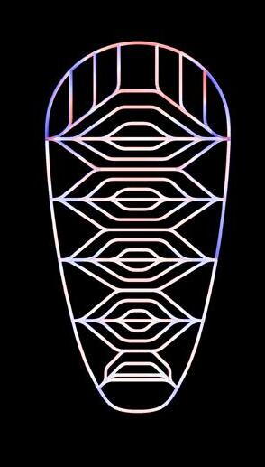
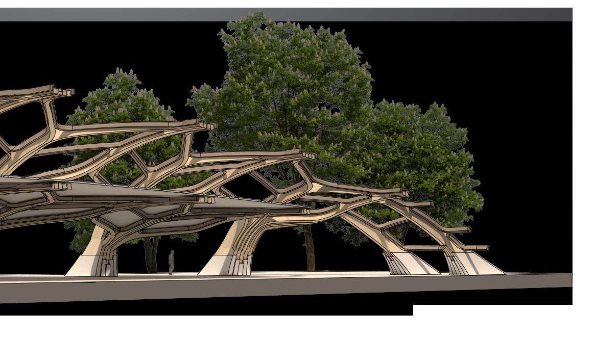
Fig. 3.13 Continuous Surface with Projected Branching System

Drawing by author, design studio drawing